Assessing Social and Territorial Vulnerability on Real Estate Submarkets

Architecture and Design Department, Politecnico di Torino, Castello del Valentino, V.le Mattioli 39, 10125 Torino, Italy
*
Author to whom correspondence should be addressed.
Buildings 2017, 7(4), 94; https://doi.org/10.3390/buildings7040094
Submission received: 28 July 2017
/
Revised: 12 October 2017
/
Accepted: 16 October 2017
/
Published: 24 October 2017
(This article belongs to the Special Issue Real Estate Economics, Management and Investments)
Abstract
:The concept of social vulnerability is widely studied in literature in order to identify particularly socially fragile sectors of the population. For this purpose, several studies have adopted indexes to measure the economic and social conditions of the population. The aim of this paper is to investigate the link between social and territorial vulnerability and the real estate market, by means of an exploratory analysis related to the possibility that spatial analyses can help to identify spatial latent components and variables in the process of price determination. A three phase approach is proposed, using the geographical segmentation of Turin and its related submarkets as a case study. After the identification and analysis of a set of three social and territorial vulnerability indicators, a traditional hedonic approach was applied to measure their influence on property listing prices. Subsequently, spatial analyses were investigated to focus on the spatial components of the indicators and property prices; their spatial autocorrelation was measured and the presence of spatial dependence was taken into account by applying a spatial regression. Results demonstrated that two indicators were spatially correlated with property prices and had a significant and negative influence on them. The proposed approach may help not only to identify the most vulnerable urban areas characterized by the lowest property prices, but also to support the future modification to the actual geographical segmentation of Turin.
1. Introduction
Urban changes are interconnected and in constant flux: economic trends, such as property price fluctuations in the real estate market, as well as social changes related to the population size and inhabitant characteristics are directly linked to processes of urban transformation. The built environment reflects all these economic and housing trends, and displays new markets, new demands and social vulnerabilities in emerging city features. The most distressed urban areas, that might be located in marginal areas or in historical city centres, have to be identified and analysed in order to monitor social and economic trends. The identification of these fragile areas can be supported by the creation and the application of specific indexes and indicators able to represent significant socio-demographic characteristics of a population and to highlight new social trends.
The aim of this paper is to investigate the link between social and territorial vulnerability and the real estate market, by means of an exploratory analysis related to the possibility that spatial analyses can help to identify spatial latent components and variables in the process of price determination. To identify the urban areas where the most fragile groups of the population are concentrated, we identified a set of three social and territorial vulnerability indicators and we analysed them for the city of Turin. We calculated the three indicators by extracting available open data related to the 3713 census cells of the city of Turin from the data warehouse of the 15th Population and Housing Census, implemented in 2011 by the Italian National Institute of Statistics (ISTAT). Subsequently, we applied a traditional hedonic model to measure the influence on property listing prices (LP) of the three indicators and physical characteristics of buildings and apartments. This second analysis was performed using a sample of 773 property listings in Turin published in 2011–2012 on one of the main Italian real estate advertisement websites. Finally, spatial analyses were investigated to focus on the spatial components of the significant indicators and property prices. Spatial autocorrelation was calculated by measuring the local spatial association level between each territorial unit and the neighbouring ones. Spatial autocorrelation analysis allowed us to measure the level of interdependence for each of the territorial units concerned and to show the types of spatial clustering of the indicators. By means of Local Indicator of Spatial Association (LISA) we identified those clusters recognized as the urban areas with the highest autocorrelation of high values (hot spots) and low ones (cold spots). Furthermore, a spatial regression was applied in order to take into account the presence of spatial dependence. The spatial analyses results showed that two indicators were spatially correlated with property prices and had a significant and negative influence on them.
2. Background
The creation and adoption of social indexes and indicators in order to identify, evaluate or rank territorial units (from a national scale up to a regional, urban or district one) is widely recognised in literature [1]. In particular, in several studies the socio-demographic and territorial characteristics are deeply analysed and combined to represent and measure different aspects of the social condition, such as: social well-being and quality of life [2,3,4,5,6,7,8,9]; social capital [10,11,12]; human development and economic inequality [13,14,15,16,17,18]; social inclusion [19,20,21].
In particular, we focused our attention on the concept of social vulnerability, which is widely studied in literature in order to identify the particularly socially fragile sectors of the population which are usually more heavily impacted by environmental hazards [22,23,24,25,26,27].
We decided not to further explore the vulnerability of territories, but to focus our attention on the construction of indexes aimed at measuring the economic and social conditions of the population. For example, de Mello Rezende [27] calculated a social vulnerability index by using a set of 23 indicators, arranged in five subjects (conditions of breadwinners, family conditions, housing conditions, urban infrastructure and economic dimension) and inserted the results in the geographic information system through ArcGis software for the spatial representation of social vulnerability levels. In [26] another social vulnerability index was constructed on the basis of a set of 14 indicators aggregated in 4 dimensions (social, education, housing and social dependence): they considered vulnerability as being composed by variation in age, gender, unemployment, dependence and property variables.
In the Italian background we found a limited number of studies concerning social vulnerability. Torre et al. [28] investigated disease conditions of the inhabitants by taking into account some structural characteristics of the population (people over 65 years and under 14; people looking for their first job and unemployed; number of entrepreneurs and professionals; number of employees, employers and self-employed workers; the number of families in relation to the size of the household; housing in relation to the property deed; territorial density) and by calculating a social weakness index.
Furthermore, a social and material vulnerability index was created by ISTAT (http://ottomilacensus.istat.it/) with the aim of measuring the exposure of some sectors of the population to uncertain social and economic conditions at the municipality scale. In this study, seven indicators were defined, according to the following main dimensions: education level, family composition, housing conditions, integration into the labor market and economic conditions.
In the present study we considered the social vulnerability as a potential uncertain condition from a social and economic point of view as being able to characterize segments of the population and, as a consequence, to influence the housing submarkets of the urban areas where these people live [29,30].
A similar approach was developed by Armaş and Gavriş [26], who constructed a census based social vulnerability index for Bucharest and explored the spatial clustering of vulnerability by means of LISA [31]. Our study goes further since we also applied a traditional hedonic approach, in order to empirically measure the influence of three social and territorial vulnerability indicators and the main apartment and building features on property listing prices.
3. Methodology
The proposed approach is based on three phases:
- Analysis of open census data available for each census cell and identification of a set of three social and territorial vulnerability indicators to identify the urban areas where the most fragile groups of the population are concentrated;
- Traditional hedonic model to measure the influence on property prices of the three indicators and some physical characteristics of buildings and apartments;
- Spatial analyses to focus on the spatial components of the significant indicators and property prices and to show the related types of spatial autocorrelation (LISA).
It is important to underline that the first phase (identification of three social and territorial vulnerability indicators) produced results that allowed us to carry out the second phase (traditional hedonic model) and the third one (spatial analyses).
3.1. Analysis of Open Census Data on Social and Territorial Vulnerability
We analysed the data warehouse of the 15th Population and Housing Census, implemented in 2011 by the Italian National Institute of Statistics (ISTAT) and we extracted open data on the website [32] for each census cell, to identify the most fragile sectors of the population from a social and economic point of view and the related urban areas where they are concentrated.
ISTAT defined seven indicators [33] in order to create a social and material vulnerability index. We analyzed them and decided to further explore some of the indicators available in the form of open data at the census cell scale. In addition, we decided to analyze other aspects in order to specifically study the link between social and territorial vulnerability and the real estate market. On this basis we decided to focus our attention on the following three issues: population’s low education level, unemployment and the presence of foreigners.
In more detail we selected 11 census data variables: literate inhabitants (without any qualifications), illiterate inhabitants, people with a primary school certificate, people with a middle school certificate, unemployed inhabitants over 15 years of age who are looking for a new job, inhabitants who are not part of any workforce, foreigners from Europe, Africa, Asia, America and Oceania living in Italy. We then aggregated the variables, which significantly and negatively influenced property prices into a set of three indicators. The process we adopted is based on the following stages: selecting census data variables, standardization, development of a first set of indicators, verification and modification, and finally the development of a final set of three indicators as follows:
- Low Education Population Indicator (LEPI): percentage of the number of literate and illiterate inhabitants, and people with primary/middle school certificate;
- Unemployed Population Indicator (UPI): percentage of unemployed inhabitants over 15 years of age who are looking for a new job;
- Foreign Population Indicator (FPI): percentage of foreigners from Africa and America living in Italy.
We standardized the considered census data variables, putting them in relation to the total number of inhabitants for each census cell. This final set of three indicators, calculated for each territorial unit, constituted the data set to be analysed by applying a traditional hedonic model and spatial analyses.
It is important to underline that in future studies the availability of additional ISTAT data would enhance the research by providing other significant indicators.
3.2. The Hedonic Model (OLS)
A traditional hedonic approach was applied in order to measure the influence of the set of three social and territorial vulnerability indicators in the real estate market [34]. In Italy transaction prices are not easily usable since they are not public information, so we had to use listing prices with all the limitations that these represent [35]. The listing price trend plays a primary role in the Italian real estate market framework. Nevertheless recent studies showed that the use of listing prices for studying the real estate market and estimating house values is viable. This is due to the fact that agents and sellers tend to correctly determine property prices and predict the influence of observable characteristics of buildings and apartments in the process of price determination [35,36,37,38,39].
Firstly, we tested the correlation between prices and the three indicators and we applied a standard hedonic regression to measure the overall influence on LP of the three indicators and the main observable attributes. The hedonic model takes the following form:
where Y is the logarithm of LP, is the model intercept, the explanatory variables , k = 1,…,K and , m = 1,...,M are the dummy variables introduced for any of the n observable characteristics, the hedonic weights and assigned to each dummy variable is equivalent to the contribution of the single characteristic level to the price value [40], and ε the error term.
In this paper, we considered unit prices measured in Euro per square meter. Empirical evidence showed that the use of unit prices improved the fit of the model [41], since the explanatory variable “apartment dimension” is able to strongly influence the process of price determination and partially decrease the influence of the other explanatory variables considered in the model. Furthermore, in Italy house prices are commonly measured in Euro per square meter by buyers, sellers and real estate institutional web sites. We therefore decided to consider the variables’ influence on prices measured in Euro per square meter, as outlined in other studies, which analysed the Italian real estate market [35,36,37,38,39,42].
The explanatory variables included in hedonic model (1) concern building characteristics and apartment characteristics that can be deduced from web advertisements.
The hedonic weights in Equation (1) were estimated using traditional least squares estimates. The coefficient of determination of the regression model (Adjusted R2) measures the proportion of variation of the dependent variable (logLP) explained by the model.
3.3. Spatial Analyses
The spatial analyses on the significant indicators and property prices consist of two steps. Firstly the spatial autocorrelation for the analysis of the indicators and property prices across the geographical units is calculated to measure the local spatial association level between each territorial unit and the neighbouring ones. Secondly, a spatial regression is used to take into account the presence of spatial dependence [43].
We used the ArcGIS software package (software version 10.2, Esri, Redlands, CA, USA) to generate the descriptive maps of the indicators. We then exported the shape file from ArcGIS to GeoDa environment for advanced geospatial analyses. GeoDa is the latest software tool devised by the Centre for Spatially Integrated Social Sciences (CSISS) to implement various exploratory spatial data analyses including data manipulation, mapping and spatial regression analysis [44].
3.3.1. Spatial Autocorrelation Analysis
Housing markets are characterized by two features: market segmentation [45,46] and spatial autocorrelation in property price [47,48].
It is commonly observed that spatial data are not independent, but rather spatially dependent, which means that observations from one location tend to exhibit values similar to those from nearby locations [49].
In this study, the spatial autocorrelation was measured and Moran scatter plot and Local Indicator of Spatial Association (LISA) were calculated [31].
The Moran scatter plot produces a graphic representation of spatial relationships and the identification of possible local clusters.
The graph represents the distribution of the statistical unit of analysis (Figure 1): the horizontal axis shows the normalized variable (y), and the normalized ordinate spatial delay of that variable (Wy). The second and fourth quadrants represent areas of values with positive correlations or spatial association of similar values (both values above or below the mean) while the first and third quadrants represent areas with negative correlation, spatial association of dissimilar values (one value above and one value below the mean) [31,49,50].
The Moran Scatter plot gives no information on the significance of spatial clusters but it permits us to identify outliers present in the statistical distribution by observing their distance from the mean and the row-standardized spatial weights matrix [31]. The significance of the spatial correlation measured through Moran’s I and Moran Scatter plot is highly dependent on the extent of the study area and on the choice of the territorial unit.
Subsequently we used Local Indicators of Spatial Association (LISA) to investigate the significance of spatial clusters. Using GeoDa software, we generated a “weight matrix” which is essential for the computation of spatial autocorrelation statistics. A wide range of criteria may be used to define neighbours, and we chose the queen contiguity first order to estimate all the geo-spatial statistics and geo-spatial regression.
The LISA is a statistic that indicates the extent of significant spatial clustering of similar values around an observation. It also allows the type of local autocorrelation to be calculated and highlights the spatial effects related to the studied phenomenon [31,52]. It is important to underline that the spatial clusters obtained with LISA do not include all those areas which present the highest values of the studied phenomenon, since the LISA calculates the contiguity with the neighbouring territorial units and their similar or dissimilar values in order to determine the formation of a cluster [31,51,53,54].
This index can be locally interpreted as an equivalent index of Moran. The sum of all the local indices is proportional to the value of the Global Moran indicator of spatial association [31].
The Local Moran’s Index is calculated as follows:
where zi is the standardized spatial weight and the summation over j is such that only neighbouring values are included. For ease of interpretation, the weights may be in row standardized form, and by convention .
The Local Moran’s I and its standardized z-score, computed by subtracting the expected value and dividing by the standard deviation provides an assessment of the similarity of each observation with that of its surroundings, for each location [52,55].
Five scenarios emerge, as described also in [51]:
- Locations with high values of the phenomenon and a high level of similarity with its surroundings (high-high), defined as “hot spots”;
- Locations with low values of the phenomenon and a high level of similarity with its surroundings (low-low), defined as “cold spots”;
- Locations with high values of the phenomenon and a low level of similarity with its surroundings (high-low), defined as “potential spatial outliers”;
- Locations with low values of the phenomenon and a low level of similarity with its surroundings (low-high), defined as “potential spatial outliers”;
- Locations devoid of significant autocorrelations.
LISA can effectively measure the degree of spatial association relative to its surroundings for each territorial unit, showing the type of spatial concentration for the detection of spatial clusters.
3.3.2. Spatial Regression models
When the “location” or “spatial” effects are ignored using Ordinary Least Squares (OLS) in linear regression analysis, the estimates are biased. The assumption of independent error terms is violated since spatial dependence and spatial autocorrelation exist in the data. Spatial autocorrelation stems from “similarities” between neighbouring clusters; there is autocorrelation when the covariance between “neighbouring” clusters is not equal to zero, and otherwise there is no autocorrelation presence [56].
Tests for spatial autocorrelation for a single variable are based on the magnitude of an indicator that combines the value observed at each location with the average value at neighbouring locations (Spatial Lags). Basically, the spatial autocorrelation tests are measures of the similarity between association in values (covariance, correlation or difference) and association in space (contiguity). Spatial autocorrelation is considered to be significant when the spatial autocorrelation statistic takes on an extreme value, compared to what would be expected under the null hypothesis of no spatial autocorrelation. When significant spatial autocorrelation exists either globally or locally, spatial heterogeneity exists [49,52].
Spatial effects are tested using the Breusch Pagan test [57] for testing homogeneity assumption, the Moran test, Lagrange Multiplier (LM) lag test and LM-error tests for testing spatial autocorrelation [56].
When spatial autocorrelation exists, the error term has to take this autocorrelation into account. We used the a spatial regression model, namely Spatial Lag Model (SLM) that takes the following form:
where, is the spatial observed value lag coefficient, and is random error for location i.
4. Location of the Most Vulnerable Sectors of the Population and Real Estate Market in Turin
The importance of market segmentation for price prediction is confirmed in [58], and is empirically supported by [36,37], who analysed the city of Turin.
We focused on the city of Turin whose territory can be actually segmented into 40 Microzones, 93 Historical Territorial Units (HTU) and 3713 census cells. The Microzones, defined in 1999 by Politecnico di Torino, were approved by the Municipal Council in accordance with DPR 138/98 and the Regulation issued by the Ministry of Finance. According to the Regulation, a Microzone is normally an area of the municipal territory which is uniform with regard to town planning and at the same time is also a segment of the real estate market.
In the last few years the Politecnico di Torino carried out some studies in order to prepare an eventual future update of the actual Microzones. In particular, in 2011 an approach based on an urban and historical analysis was developed in order to specify the Microzones into 93 smaller areas (HTU).
The Microzones were established by considering price levels, building characteristics, accessibility, presence of services and green areas, whereas the HTUs were defined on the basis of urban areas and building characteristics, such as urban and environmental features, building construction period and property quality level [59,60]. The relation between Microzones and property prices has been deeply studied in several studies [36,37], while the HTU’s influence in the real estate market has been recently analysed in [38] but needs to be more investigated.
In order to analyse the variability of the social issues represented by areas where the most vulnerable sectors of the population live and their link with the real estate market, we used the HTU territorial segmentation. On this basis future studies can be directed to further explore the actual Microzones by taking into account the historical features of the built environments that the HTUs represent. In particular, future research may be directed to verify and modify the actual boundaries of the Microzones and the HTUs or it could also take into account the possible aggregation of smaller Microzones and the segmentation of the bigger ones.
4.1. The 2011 ISTAT Data: Turin Population Sample
We based the analysis of the set of three social and territorial vulnerability indicators on a sample of open data extracted from the data warehouse of the 15th Population and housing census, implemented in 2011 by ISTAT and containing a wealth of information, at a sub municipal level (census cells), about the demographic and social structure of the population resident in Turin and in the related housing stock. ISTAT is a public research organization: it has been present in Italy since 1926, and is the main producer of official statistics in the service of citizens and policy-makers. It operates in complete independence and continuous interaction with the academic and scientific communities [32].
In particular, we selected the following census data variables: inhabitants with a middle school certificate; inhabitants with a primary school certificate; literate inhabitants (without any qualifications); illiterate inhabitants; unemployed inhabitants over 15 years of age who are looking for a new job; unemployed inhabitants over 15 years of age who are not part of any workforce; foreigners from Europe, Africa, Asia, America and Oceania living in Italy; total number of inhabitants (Table 1).
4.2. The Turin Property Prices Sample: Data and Descriptive Statistics
To apply the hedonic model to measure the influence of the three indicators on house prices, we based the study on a sample of 773 property listings in Turin published in 2011–2012 on one of the main Italian real estate advertisements websites. We chose to analyse data collected in 2011–2012, in coherence with the Turin population sample, based on the 15th Population and Housing Census, implemented in 2011 by ISTAT. The dataset was selected from a database of 978 data, from which we eliminated the outliers, the observations with missing addresses and those sited in villas and multi-family dwellings, as well as apartments sited on the ground floor and in the attic. The sample belongs to a database property of the Turin Real Estate Market Observatory [61], that was founded in 2000 to monitor the Turin real estate market on the basis of the segmentation in Microzones [62].
The LP mean price of our sample is 2666 Euro per square metre with a standard deviation of 1085 Euro per square metre. The variables considered in the model included building characteristics and apartment characteristics.
For each sampled apartment put up for sale we considered the characteristics of buildings and apartments listed in Table 2, explaining the type of variables and the descriptive statistics for each characteristic. The variable BCP has been constructed by defining three periods according to the three main phases of Turin’s urban development: it is important to highlight that, like most of the Italian cities, the Turin building stock mainly consists of buildings built during the Post—World War II period and historical ones.
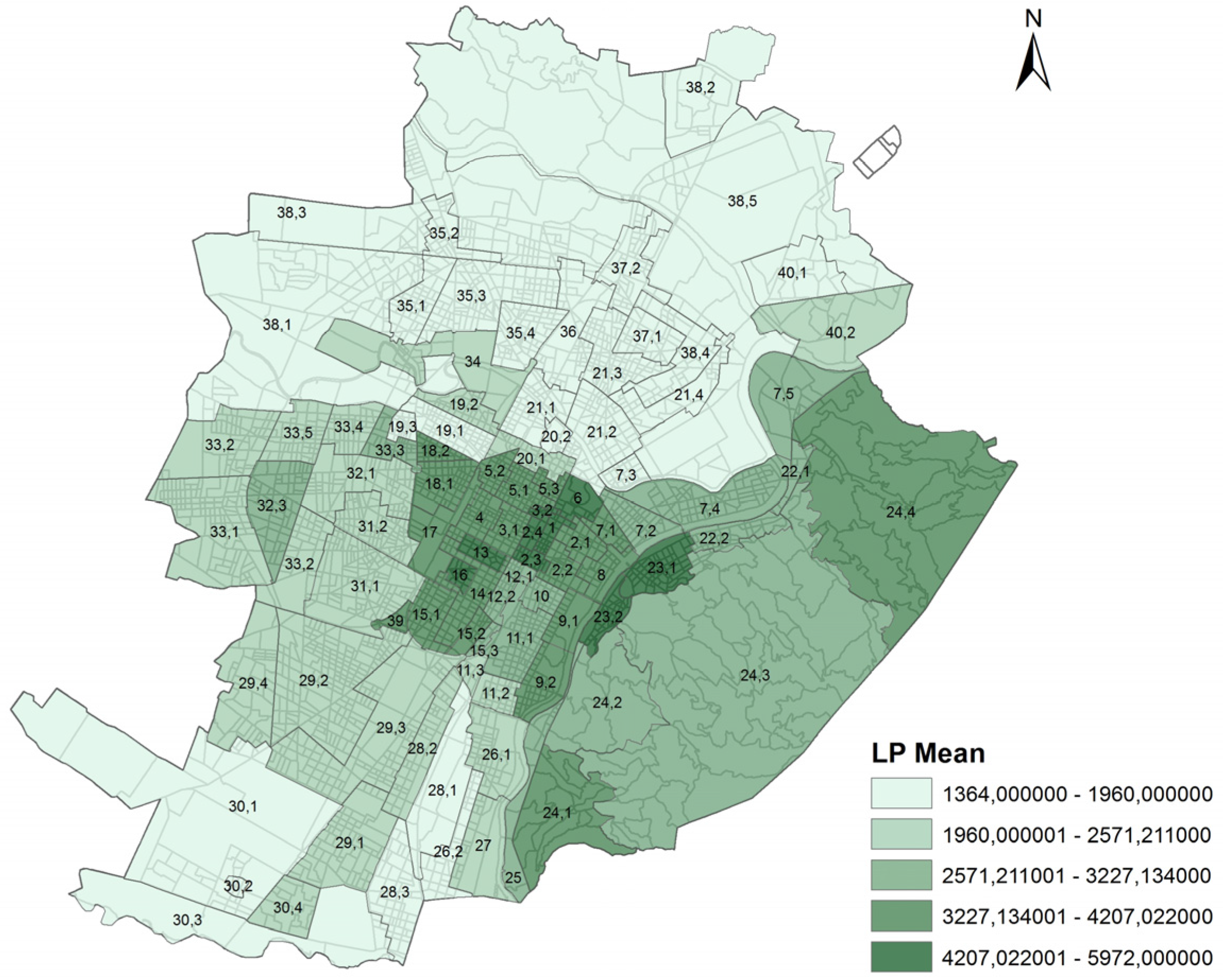
In order to proceed with the third phase of the proposed approach (spatial analyses) we built a dataset that included the location, specified using the above mentioned geographical segmentation in Historical Territorial Units (HTU): the frequency of each indicator and price means were calculated for each HTU. Figure 2 shows the sample size and the price means in the 93 HTUs.
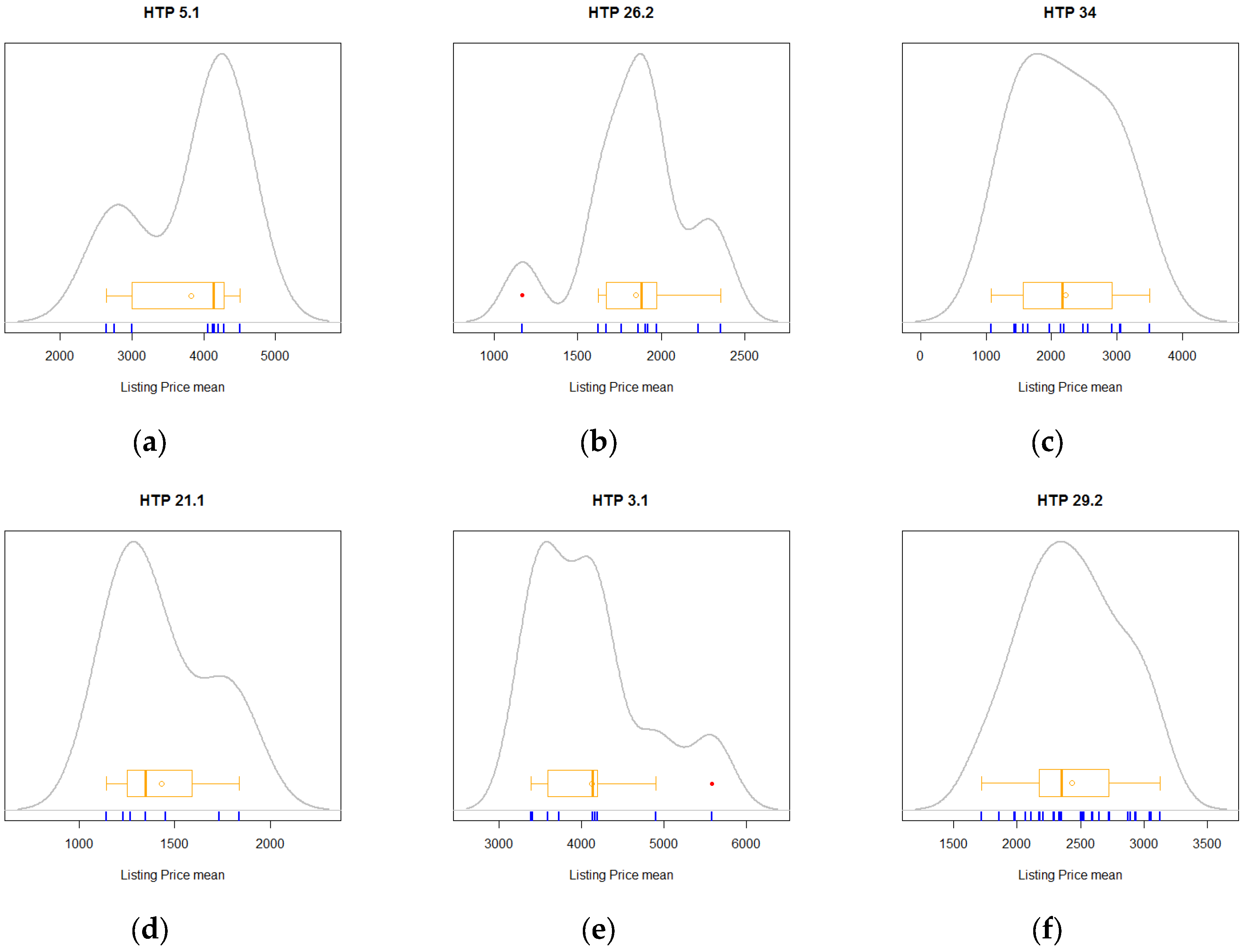
For those HTUs which presented statistically significant samples we provided the Kernel density plot and the LP box plots: some examples in Figure 3 show that each HTU presents a different distribution of the LP variable. It is important to underline that the frequency of the observations in each of the territorial units obviously affects the density curve: huge samples more frequently present a normal distribution.
5. Results
5.1. Social and Territorial Vulnerability Indicators
On the basis of the Turin population sample described in Section 4.1, extracted from the data warehouse of the 2011 ISTAT data—15th Population and Housing Census, we calculated the three indicators for each of the 3713 census cells. The Low Education Population Indicator (LEPI), Unemployed Population Indicator (UPI) and Foreign Population Indicator (FPI) are differently represented throughout the whole city. The LEPI ranged from 0.00 to 1.00, with an average score of 0.48. The UPI ranged from 0.00 to 0.67 with an average score of 0.03, while the FPI ranged from 0.00 to 1.00 with an average score of 0.05.
5.2. The Hedonic Model Results
The dependent variable of the hedonic model represented the apartments listing price (LP), measured in Euro per square meter. Before applying the hedonic analysis we tested the normality of the LP variable. The test rejected normality, even after removing the outliers (with a p-value p < 0.05). We therefore transformed the LP variable into a logarithmic variable (logLP). We repeated the test which then did not reject the null hypothesis.
We therefore applied the regression model (1) outlined in Section 3.2 to assess the overall influence of the three indicators on property prices. In addition to the three indicators, the set of explanatory variables employed in the hedonic model included some physical observable features (apartment characteristics and building characteristics) [63]. Results are shown in Table 3.
By analysing the results it is possible to notice that the model was able to explain 69% of the price variation (Adjusted R2 = 69%) and that only two indicators (LEPI and FPI) significantly influenced the property price determination process.
Furthermore, the model showed that the variables “building quality” and “apartment condition” significantly influenced price values. On the contrary, other variables such as the building typology, the Energy Performance Certificate (EPC) label and the presence of a lift had a low influence on prices and for this reason they were not included in the model [39,42].
We then tested the correlation between the dependent variable and the three indicators: the results showed a high negative correlation between them. The correlation analysis identified LEPI as the component that was more correlated to the dependent variable (Table 4).
It is important to underline that the OLS model was applied with a descriptive purpose, since the spatial dependence was not investigated at this first stage. A second stage was therefore devoted to this aim by using a spatial regression on a sample of data aggregated for the 93 Historical Territorial Units (HTUs) and focusing the attention on the social and territorial vulnerability indicators.
5.3. Spatial Analyses in the 93 Historical Territorial Units (HTUs)
We decided to analyse the spatial component of the two indicators that significantly influenced the process of property price determination (LEPI and FPI). These two indicators and the property listing prices, calculated for each HTU, constituted the data to be analysed by means of spatial analyses.The trends in listing prices and in the two indicators are presented in Figure 4.
The trends suggested a correlation between the pattern of the price means in the HTUs and the pattern of LEPI. Overall the proportion of LEPI varies between 22 percent in the city centre and on the hills and rises to 70 percent in the northern and southern areas of the city. The proportion of FPI varied between 1 percent and 17 percent in the urban area between “Piazza della Repubblica” and “Borgata Monterosa”.
By means of spatial autocorrelation analyses (LISA) we firstly identified spatial clusters that represented the highest concentration of the most and least vulnerable population. Secondly, a spatial regression was applied to take into account the presence of spatial dependence.
5.3.1. Spatial Autocorrelation Analysis
We calculated Moran’s I, Moran Scatter plot and Local Indicators of Spatial Association (LISA), detailed in Section 3.3, by using the HTU as territorial minimum unit.
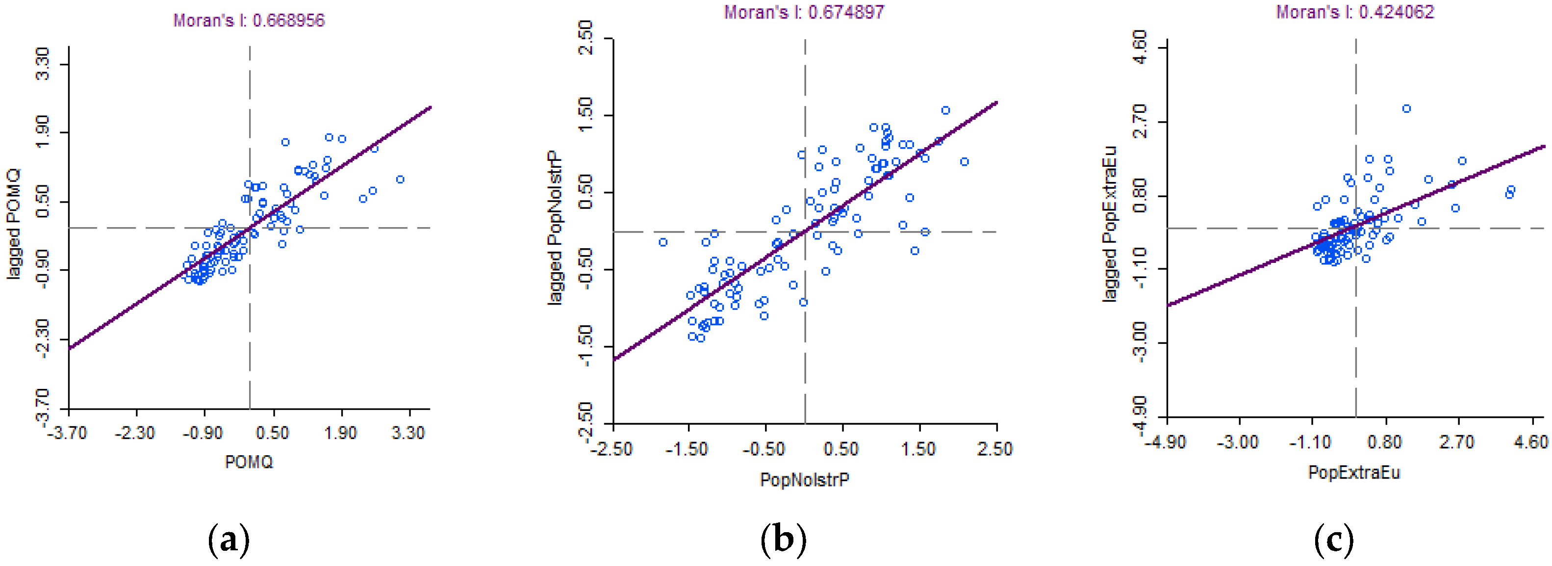
Moran’s I and Moran Scatter Plot Results
To account for the magnitude of geo-spatial clustering among the dependent and the explanatory variables, we calculated the Moran’s I statistics for each of the variables. The results are presented in Figure 5. The findings suggest geo-spatial clustering in the dependent and explanatory variables and the highest value of autocorrelation (Moran’s I = 0.675) was observed for the variable LEPI.
The Moran scatter plot allowed us to verify the presence of a positive autocorrelation across the HTUs since most of the observations were located in the I and III quadrant. There were also some hypothetical outliers with data that were distant from the mean in the III quadrant.
LISA Results
We subsequently calculated LISA for the dependent and the explanatory variables in the 93 HTUs and examined the spatial relationship between them. The calculation of significance (99 permutation) processed by GeoDa on the basis of Monte Carlo statistics confirmed the significance of the clusters, with a p-value of between 0.001 and 0.05 [64].
The LISA results for listing price and the two indicators are presented in Figure 6.
Findings suggest striking geographic clustering of property prices in the central, northern and southern urban areas. A first cluster, located in the north and in the south areas of the city, represented the urban areas characterized by a positive autocorrelation of high values and high level of similarity with its surroundings (High-High). A second cluster, located in the city centre and on the hills, represented the urban areas characterized by the positive autocorrelation of low values and high level of similarity with its surroundings (Low-Low).
A similar clustering was observed in the case of the low education population: in particular it is possible to notice a certain reverse correspondence between the spatial clusters obtained for property prices and those obtained with LEPI: the LEPI High-High LISA Cluster corresponds to the LP Low-Low LISA Cluster, and vice versa.
The northern area is also characterized by a high concentration of African and American nationals living in Italy, identified by a smaller cluster of HTUs that are between “Piazza della Repubblica” and “Borgata Monterosa”.
The results presented in Figure 6 provide compelling evidence that the urban areas characterized by low education level inhabitants were also more likely to record low price housing rates. Furthermore, the findings suggested that the HTUs of the north part of the city are marked by a strong presence of the population with a low education level and a large number of African and American nationals living in Italy.
5.3.2. Spatial Lag Model
We applied the Spatial Lag Model (3) outlined in Section 3.3.2 to assess the influence of LEPI and FPI on property prices. The dependent variable represented the apartments LP, measured in Euro per square meter and transformed in its logarithmic form.
Since we found considerable geo-spatial clustering in the dependent and explanatory variables, we presented both the results of the OLS model and Spatial Lag model, used to assess the association between logLP and LEPI and FPI (Table 5).
We presented the results of the Spatial Lag model to account for the geo-spatial clustering in the dependent and explanatory variables. Findings revealed the improvement of the model with the introduction of the spatial variable (W) with a R-squared rising from 0.822 to 0.875. Findings also suggested that a low education level population and the presence of foreigners—represented by the two indicators—were spatially correlated with property values and had a significant and negative influence on them.
The results showed the considerable explanatory power of the indicators, which can also be considered proxies of other physical and territorial features. Future studies may therefore be oriented to further explore not only the influence of the social and territorial vulnerability indicators, but also the effects deriving from their interactions.
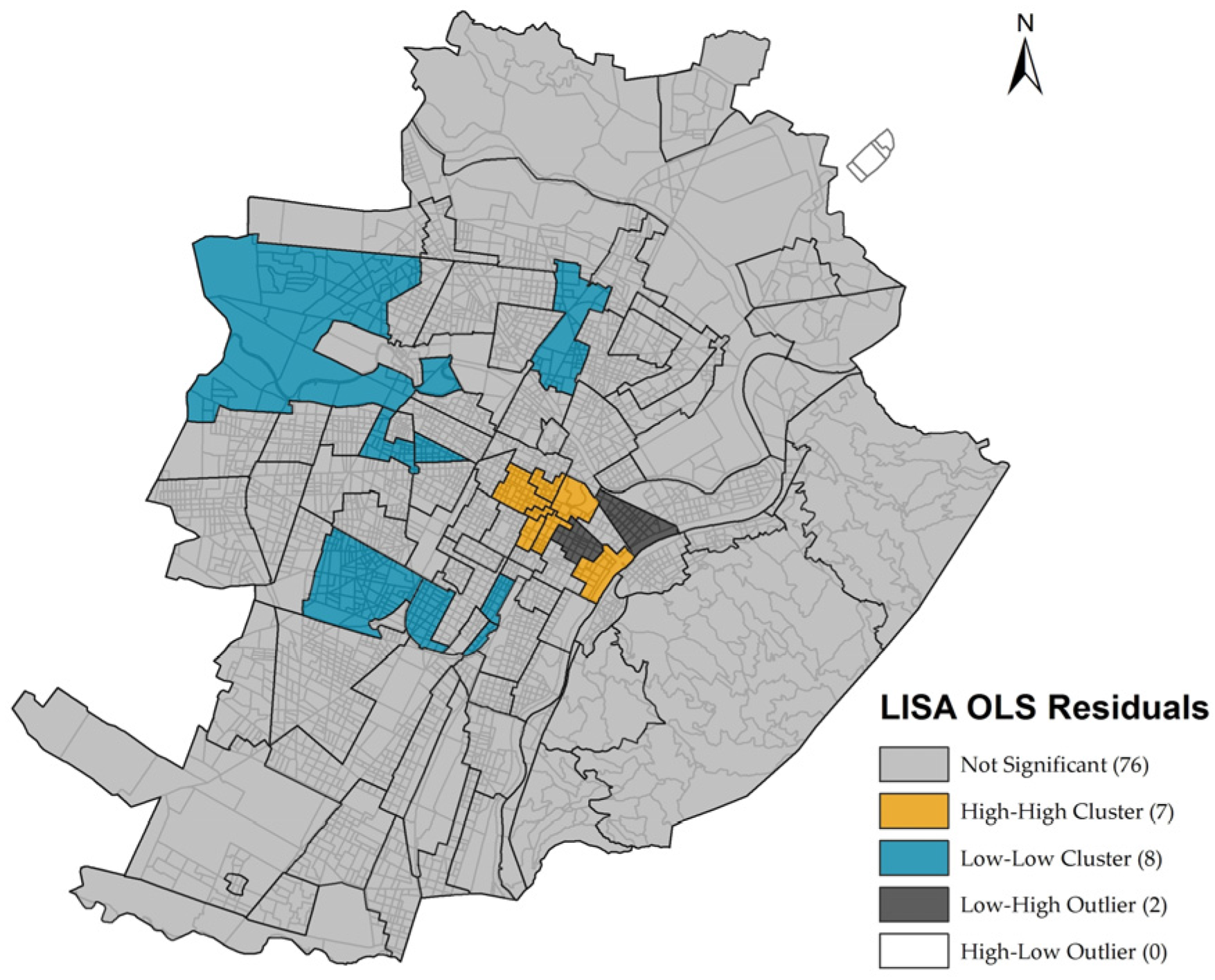
Subsequently we measured the spatial autocorrelation detected in the residuals of the hedonic pricing model. The OLS residual pattern, showed in Figure 7, revealed the absence of autocorrelation in 76 HTUs.
As expected, the High-High cluster included 7 HTUs located in the city center, which is characterized by low values of vulnerability and high property prices. On the contrary, the Low-Low cluster included 8 HTUs located in different urban areas of the city. For example, the HTU in the western side is characterized by different building typologies and by the presence of the Dora river that delimits specific territorial segments. This could mean that some HTUs are not homogeneous since they include areas with different urban and environment features and also historical buildings that are heterogeneous considering their typology and condition level. Furthermore, the real estate market may not work equally in all the HTUs; above all in contexts characterized by low price trends the stochastic components play a primary role. We can therefore conclude that the OLS residuals are not correlated with LEPI and FPI, but with other physical or territorial variables—not included in the spatial regression model—that need to be further explored.
6. Conclusions
The concept of social vulnerability has been widely studied in literature. We introduced an analysis within the context of real estate submarkets. We identified and analysed a set of three social and territorial vulnerability indicators representative of the most fragile sectors of the population in the city of Turin. We based our analysis on a sample of open census data available for each census cell, which allowed us to study 11 census variables and to aggregate those which significantly and negatively influenced property prices into a set of three indicators.
The hedonic model results showed that only two indicators (LEPI and FPI) had a significant and negative influence on property prices. This means that a concentration of low education population and/or of foreigners influenced the real estate market.
Subsequently, spatial analyses were investigated to focus on the spatial components of the two indicators LEPI and FPI and property prices. By measuring the spatial autocorrelation of property prices with the Local Indicator of Spatial Association (LISA) we found that the areas characterized by positive autocorrelation of high house prices usually presented low values of LEPI and vice versa. In particular, we identified two spatial clusters. The first cluster, located in the north and in the south areas of the city, represented the urban areas characterized by the positive autocorrelation of high values of LEPI (hot spots).The second cluster, located in the city centre and on the hills, represented the urban areas characterized by the positive autocorrelation of low values of LEPI (cold spots).
Finally, we applied a spatial regression in order to take into account the presence of spatial dependence. The spatial analyses results showed that the two indicators were spatially correlated with property prices and had a significant and negative influence on them.
Starting from our study, further researches can be developed, analysing and comparing the social and territorial vulnerability of different cities or repeating the present analysis by using samples from other years. Furthermore, the proposed approach may help not only to identify the most vulnerable urban areas characterized by the lowest property prices, but also to support the future modification to the actual geographical segmentation of Turin. Future studies can therefore be focused not only on social and territorial vulnerability but also on its relations with other physical and territorial variables, in order to further explore and eventually modify the actual boundaries of the Microzones and the HTUs.
Limitations of the Study
One of the key limitations of the analysis was the non-availability of information at the census cell scale, such as the inhabitants’ incomes, the number of inhabitants who live in highly crowded residential units, the number of vulnerable inhabitants who need social and welfare assistance. Several recent studies have highlighted the importance of such variables in explaining the process of price determination. We could not use such variables because of they are not available at the census cell level, although at municipality and regional level they are available. It is important to underline that in future studies the availability of additional ISTAT data would enhance the research by providing other significant indicators.
Moreover, other key limitation of the analysis was the non-availability of transaction prices; we had to use a sample of listing prices, using them as a proxy of the actual transaction prices.
Author Contributions
This paper is to be attributed in equal parts to the authors.
Conflicts of Interest
The authors declare no conflicts of interest.
References
- EC (European Commission). Social Protection Committee Indicators Sub-group EU Social Indicators—Europe 2020 Poverty and Social Exclusion Target. Available online: http://ec.europa.eu/social/main.jsp?catId=756&langId=en (accessed on 27 July 2017).
- Schneider, M. The “quality of life” and social indicators research. Public Administration Review. Public Adm. Rev. 1976, 36, 297–305. [Google Scholar] [CrossRef]
- Davis, E.E.; Fine-Davis, M. Social indicators of living conditions in Ireland with European comparisons. Soc. Indic. Res. 1991, 25, 103–365. [Google Scholar] [CrossRef]
- Diener, E. A value based index for measuring national quality of life. Soc. Indic. Res 1995, 36, 107–127. [Google Scholar] [CrossRef]
- Diener, E.; Suh, E. Measuring quality of life: Economic, social, and subjective indicators. Soc. Ind. Res. 1997, 40, 189–216. [Google Scholar] [CrossRef]
- Segre, E.; Rondinella, T.; Mascherini, M. Well-being in Italian regions. Measures, civil society consultation and evidence. Soc. Ind. Res. 2011, 102, 47–69. [Google Scholar] [CrossRef]
- Andrews, F.M.; Withey, S.B. Social Indicators of Well-being: Americans’ Perceptions of Life Quality; Springer Science & Business Media: Berlin, Germany, 2012. [Google Scholar]
- Bechini, T. La disuguaglianza in Italia: Un’analisi multidimensionale per circoscrizioni. EyesReg—Giornale di Scienze Regionali 2017, 7, 64–69. [Google Scholar]
- Calcagnini, G.; Perugini, F. Un indicatore di benessere per le province italiane. EyesReg—Giornale di Scienze Regionali 2017, 7, 70–74. [Google Scholar]
- Grootaert, C.; Van Bastelaer, T. Understanding and Measuring Social Capital; The World Bank Social Development Family; Environmentally and Socially Sustainable Development Network: Washington DC, USA, 2002. [Google Scholar]
- Sabatini, F. Capitale sociale, imprese sociali, spesa pubblica e benessere sociale in Italia. Impresa Sociale 2007, 76, 192–233. [Google Scholar]
- Blokland, T.; Savage, M. Networked Urbanism: Social Capital in the City; Ashgate: Farnham, UK, 2008; ISBN 978 0 7546 7201 2. [Google Scholar]
- Atkinson, A.B. On the measurement of inequality. J. Econ. Theory 1970, 2, 244–263. [Google Scholar] [CrossRef]
- Sagar, A.D.; Najam, N. The human development index: A critical review. Ecol. Econ. 1998, 25, 249–264. [Google Scholar] [CrossRef]
- Monni, S. L’indice di sviluppo umano nelle province italiane. QA Rivista dell’Associazione Rossi-Doria 2002, 1, 115–131. [Google Scholar]
- Kovacevic, M. Review of HDI critiques and potential improvements. Hum. Dev. Res. Pap. 2010, 33, 1–44. [Google Scholar]
- UNDP (United Nations Development Programme). Human Development Report—Technical Notes 2016. Available online: http://hdr.undp.org/en/2016-report (accessed on 13 May 2017).
- Hirai, T. The Human Development Index and Its Evolution. In The Creation of the Human Development Approach; Springer International Publishing: Berlin, Germany, 2017; pp. 73–121. [Google Scholar]
- Atkinson, T.; Cantillon, B.; Marlier, E.; Nolan, B. Social Indicators: The EU and Social Inclusion; OUP Oxford: Oxford, UK, 2002. [Google Scholar]
- Giambona, F.; Vassallo, E. Composite indicator of social inclusion for European countries. Soc. Ind. Res. 2014, 116, 269–293. [Google Scholar] [CrossRef]
- Pollutri, S. Indicatori sintetici d’integrazione degli immigrati: Un’applicazione ai comuni marchigiani. EyesReg—Giornale di Scienze Regionali 2017, 7, 106–111. [Google Scholar]
- Cutter, S.L.; Boruff, B.J.; Shirley, W.L. Social vulnerability to environmental hazards. Soc. Sci. Q. 2003, 84, 242–261. [Google Scholar] [CrossRef]
- Rygel, L.; O’sullivan, D.; Yarnal, B. A method for constructing a social vulnerability index: An application to hurricane storm surges in a developed country. Mitig. Adapt. Strateg. Glob. Chang. 2006, 11, 741–764. [Google Scholar] [CrossRef]
- Flanagan, B.E.; Gregory, E.W.; Hallisey, E.J.; Heitgerd, J.L.; Lewis, B. A social vulnerability index for disaster management. J. Homel. Secur. Emerg. Manag. 2011, 8. [Google Scholar] [CrossRef]
- Lee, Y.-J. Social vulnerability indicators as a sustainable planning tool. Environ. Impact Assess. Rev. 2014, 44, 31–42. [Google Scholar] [CrossRef]
- Armaş, I.; Gavriş, A. Census-based social vulnerability assessment for Bucharest. Procedia Environ. Sci. 2016, 32, 138–146. [Google Scholar] [CrossRef]
- De Mello Rezende, G.B. Social Vulnerability Index: A Methodological Proposal for Application in the Cities of Barra do Garcas—MT, Pontal Do Araguaia—MT and Aragarcas—GO, Brazil. Open J. Soc. Sci. 2016, 4, 32–45. [Google Scholar] [CrossRef]
- Torre, C.M.; Morano, P.; Taiani, F. Social balance and economic effectiveness in historic centers rehabilitation. In International Conference on Computational Science and Its Applications; Springer: Cham, Switzerland, 2015; pp. 317–329. [Google Scholar]
- Whitehead, C.M.E. Chapter 40 Urban housing markets: Theory and policy. In Handbook of Regional and Urban Economics; Elsevier: Amsterdam, The Netherlands, 1999; Volume 3, pp. 1559–1594. [Google Scholar]
- Watkins, C.A. The definition and identification of housing submarkets. Environ. Plan. 2001, 33, 2235–2253. [Google Scholar] [CrossRef]
- Anselin, L. Local indicators of spatial association—LISA. Geogr. Anal. 1995, 27, 93–115. [Google Scholar] [CrossRef]
- Italian National Institute of Statistics (ISTAT). Available online: www.istat.it (accessed on 13 May 2017).
- 8milaCensus—ISTAT. Available online: www.ottomilacensus.istat.it (accessed on 13 May 2017).
- Bourassa, S.C.; Cantoni, E.; Hoesli, M. Spatial Dependence, Housing Submarkets, and House Prices. J. Real Estate Financ. Econ. 2007, 35, 143–160. [Google Scholar] [CrossRef]
- Curto, R.; Fregonara, E.; Semeraro, P. Asking Prices vs Market Prices: An Empirical Analysis. Territorio Italia 2012, XII, 53–72. [Google Scholar]
- Semeraro, P.; Fregonara, E. The impact of house characteristics on the bargaining outcome. J. Eur. Real Estate Res. 2013, 6, 262–278. [Google Scholar] [CrossRef]
- Curto, R.; Fregonara, E.; Semeraro, P. Listing behaviour in the Italian real estate market. Int. J. Hous. Mark. Anal. 2015, 8, 97–117. [Google Scholar] [CrossRef]
- Barreca, A.; Curto, R.; Rolando, D. Location and real estate values: a study of the territorial segmentation of the Microzones of Turin. Territorio Italia 2017, 1, 69–91. [Google Scholar]
- Fregonara, E.; Rolando, D.; Semeraro, P. Energy Performance Certificates in the Turin real estate market, accepted for publication. J. Eur. Real Estate Res. 2017, 10, 149–169. [Google Scholar] [CrossRef]
- Rosen, S. Hedonic prices and explicit markets: Production differentiation in pure competition. J. Political Econ. 1974, 82, 34–55. [Google Scholar] [CrossRef]
- Hoesli, M.; Morri, G. Investimento Immobiliare, Mercato, Valutazione, Rischio E Portafogli; Hoepli: Milano, France, 2010. [Google Scholar]
- Becchio, C.; Ferrando, D.G.; Fregonara, E.; Milani, N.; Quercia, C.; Serra, V. The cost optimal methodology for evaluating the energy retrofit of an ex-industrial building in Turin. Energy Procedia 2015, 78, 1039–1044. [Google Scholar] [CrossRef]
- Bourassa, S.; Cantoni, E.; Hoesli, M. Predicting House Prices with Spatial Dependence: A Comparison of Alternative Methods. J. Real Estate Res. 2010, 32, 139–159. [Google Scholar]
- Anselin, L. Exploratory Spatial Data Analysis and Geographic Information Systems. In New Tools for Spatial Analysis; Painho, M., Ed.; Euro-Stat.: Luxembourg, 1994; pp. 45–54. [Google Scholar]
- Goodman, A.C.; Thibodeau, T.G. Housing market Segmentation. J. Hous. Econ. 1998, 7, 121–143. [Google Scholar] [CrossRef]
- Goodman, A.C.; Thibodeau, T.G. Housing market segmentation and hedonic prediction accuracy. J. Hous. Econ. 2003, 12, 181–201. [Google Scholar] [CrossRef]
- Goodchild, M.F. Spatial Autocorrelation; Hutchins, C.S., Ed.; Geo Books: Norwich, UK, 1986; ISBN 0-86094-223-6. [Google Scholar]
- Basu, S.; Thibodeau, T. Analysis of Spatial Autocorrelation in House Prices. J. Real Estate Financ. Econ. 1998, 17, 61–85. [Google Scholar] [CrossRef]
- LeSage, J.P. An Introduction to Spatial Econometrics. Revue d’Economie Industrielle 2008, 19–44. [Google Scholar] [CrossRef]
- Anselin, L.; Syabri, I.; Kho, Y. GeoDa: An introduction to spatial data analysis. Geogr. Anal. 2006, 38, 5–22. [Google Scholar] [CrossRef]
- Scardaccione, G.; Scorza, F; Las Casas, G.; Murgante, B. Spatial autocorrelation Analysis for the Evaluation of Migration Flows: The Italian Case. In ICCSA 2010: Computational Science and Its Applications; Springer: Berlin/Heidelberg, Germany, 2010; pp. 62–76. [Google Scholar]
- Anselin, L. Spatial Econometrics: Methods and Models; Kluwer Academic: Dordrecht, The Netherlands, 1988. [Google Scholar]
- Barbaccia, I.; Ghiraldo, E.; Festa, M. Real estate values in low dynamic markets: Proximity effects. Territorio Italia 2012, 2, 35–69. [Google Scholar]
- Wu, C.; Sharma, R. Housing submarket classification: The role of spatial contiguity. Appl. Geogr. 2012, 32, 746–756. [Google Scholar] [CrossRef]
- Cliff, A.; Ord, J. Spatial Processes: Models and Applications; Pion Limited: London, UK, 1981. [Google Scholar]
- Haining, R.P. Spatial Data Analysis, Theory and Practice; Cambridge University Press: Cambridge, UK, 2003. [Google Scholar]
- Breusch, T.S.; Pagan, A.R. A Simple Test of Heteroscedasticity and Random Coefficient Variation. Econometrica 1979, 47, 1287–1294. [Google Scholar] [CrossRef]
- Bourassa, S.C.; Hoesli, M.; Peng, V.S. Do housing submarkets really matter? J. Hous. Econ. 2003, 12, 12–28. [Google Scholar] [CrossRef]
- Fregonara, E.; Giordano, R.; Rolando, D.; Tulliani, J.M. Integrating Environmental and Economic Sustainability in New Building Construction and Retrofits. J. Urban Technol. 2016, 23, 3–28. [Google Scholar] [CrossRef]
- Fregonara, E. Methodologies for supporting sustainability in energy and buildings. The contribution of Project Economic Evaluation. Energy Procedia 2017, 111, 2–11. [Google Scholar] [CrossRef]
- Turin Real Estate Market Observatory. Available online: www.oict.polito.it/en (accessed on 13 May 2017).
- Curto, R.; Fregonara, E. Un sistema informativo territoriale per l’osservazione del mercato immobiliare a supporto dei catasti urbani e della gestione del territorio. Quaderni CeSET. Aestimum 2002, 1, 24–60. [Google Scholar]
- Anselin, L.; Rey, S. Properties of Tests for spatial dependance in Linear Regression Models. Geogr. Anal. 1991, 23, 112–131. [Google Scholar] [CrossRef]
- Slocum, T.A.; McMaster, R.B.; Kessler, F.C.; Howard, H.H. Thematic Cartography and Geovisualization, 3rd ed.; Pearson Prentice Hall: Upper Saddle River, NJ, USA, 2009. [Google Scholar]
Figure 1.
Anselin‘s Moran scatter plot interpretation guide. (Source: Authors’ elaboration on [51]).
Figure 1.
Anselin‘s Moran scatter plot interpretation guide. (Source: Authors’ elaboration on [51]).
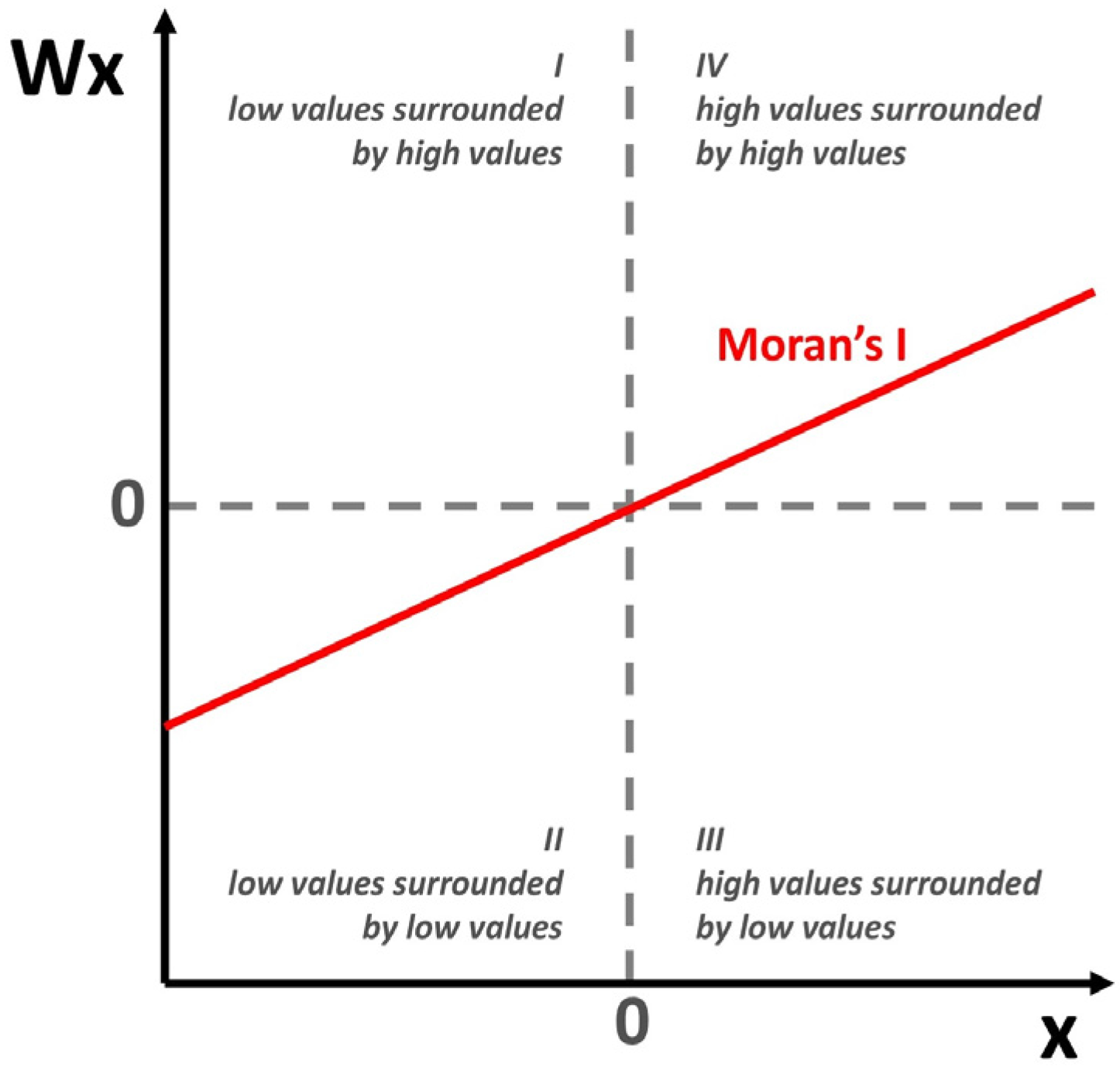
Figure 2.
The price means in the 93 Historical Territorial Units (Source: Authors’ elaboration on TREMO data).
Figure 2.
The price means in the 93 Historical Territorial Units (Source: Authors’ elaboration on TREMO data).

Figure 3.
Kernel density plot and LP box plot (measured in Euro per square metre): (a) HTU 5_1 subsample; (b) HTU 26_2 subsample; (c) HTU 34 subsample; (d) HTU 21_1 subsample; (e) HTU 3.1 subsample; (f) HTU 29.2 (Source: Authors’ elaboration on TREMO data).
Figure 3.
Kernel density plot and LP box plot (measured in Euro per square metre): (a) HTU 5_1 subsample; (b) HTU 26_2 subsample; (c) HTU 34 subsample; (d) HTU 21_1 subsample; (e) HTU 3.1 subsample; (f) HTU 29.2 (Source: Authors’ elaboration on TREMO data).

Figure 4.
Trends in the two indicators across 93 HTUs of Turin: (a) LEPI, census data of 2011; (b) FPI, census data of 2011. (Source: Authors’ elaboration).
Figure 4.
Trends in the two indicators across 93 HTUs of Turin: (a) LEPI, census data of 2011; (b) FPI, census data of 2011. (Source: Authors’ elaboration).
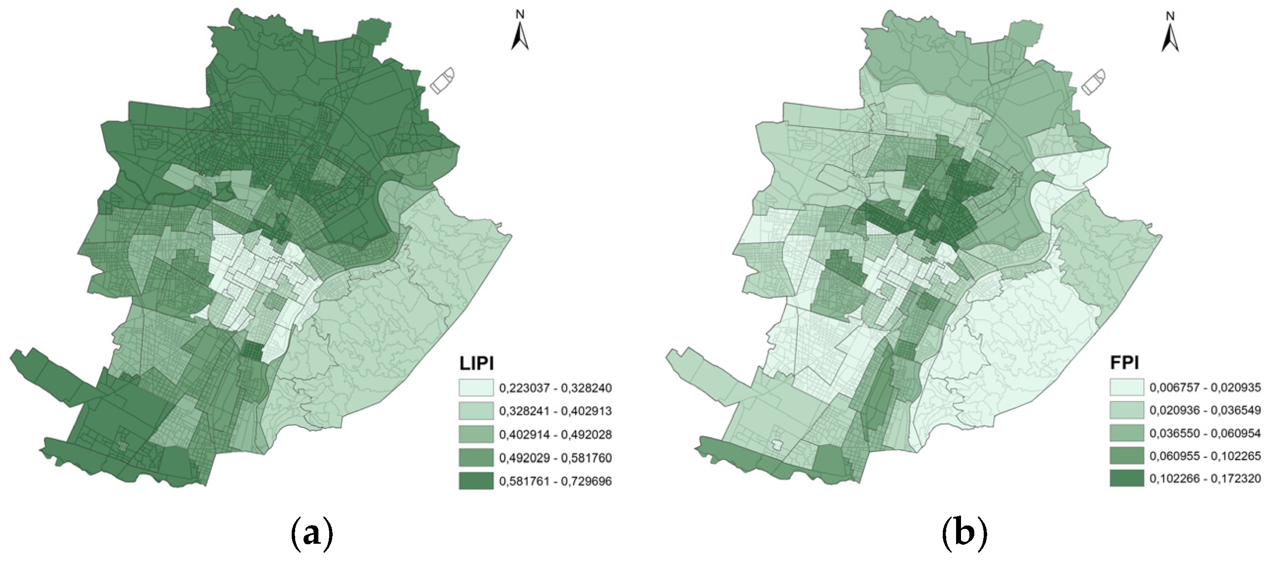
Figure 5.
Moran’s I and Moran Scatter plots: (a) LP mean; (b) LEPI; (c) FPI. (Source: Authors’ elaboration).
Figure 5.
Moran’s I and Moran Scatter plots: (a) LP mean; (b) LEPI; (c) FPI. (Source: Authors’ elaboration).

Figure 6.
LISA (Cluster and Significance) maps depicting spatial clustering and spatial outliers in the 93 HTUs of Turin, 2011: (a) LP rate, measured in Euro per square meter; (b) LEPI rate; (c) FPI rate (Source: Authors’ elaboration).
Figure 6.
LISA (Cluster and Significance) maps depicting spatial clustering and spatial outliers in the 93 HTUs of Turin, 2011: (a) LP rate, measured in Euro per square meter; (b) LEPI rate; (c) FPI rate (Source: Authors’ elaboration).
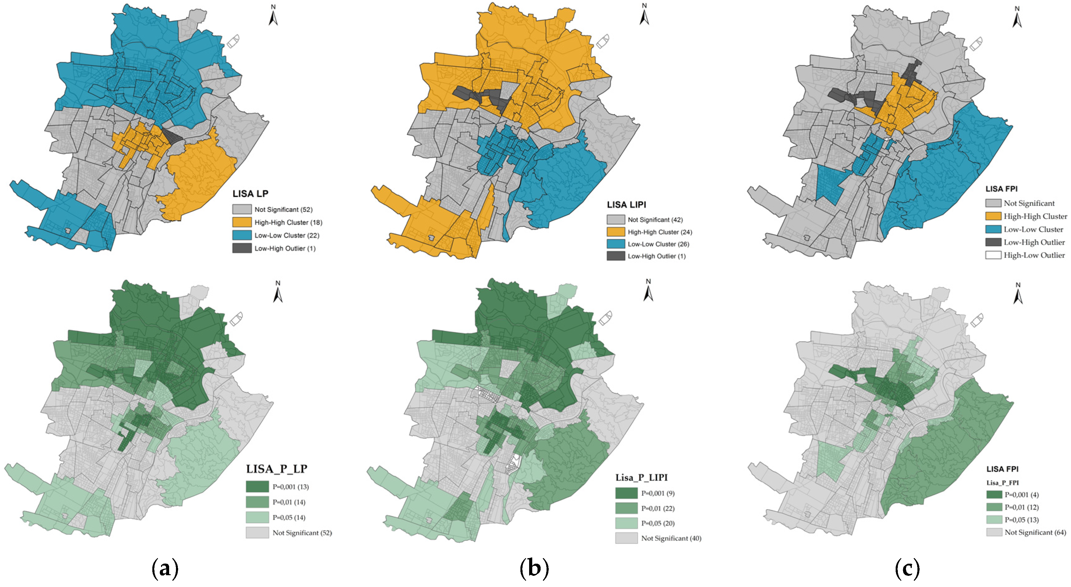
Figure 7.
LISA (Cluster) maps depicting spatial clustering and spatial outliers of OLS residuals in the 93 HTUs of Turin. (Source: Authors’ elaboration).
Figure 7.
LISA (Cluster) maps depicting spatial clustering and spatial outliers of OLS residuals in the 93 HTUs of Turin. (Source: Authors’ elaboration).

Table 1.
Turin population sample: descriptive statistics of the census data variables (Source: Authors’ elaboration on 2011 ISTAT 15th Population and housing census).
Table 1.
Turin population sample: descriptive statistics of the census data variables (Source: Authors’ elaboration on 2011 ISTAT 15th Population and housing census).
| Census Data Variables | Number | % |
|---|---|---|
| Inhabitants with a middle school certificate | 244,189 | 27.992 |
| Inhabitants with a primary school certificate | 139,508 | 15.992 |
| Literate inhabitants (without any qualifications) | 53,932 | 6.068 |
| Illiterate inhabitants | 6848 | 0.785 |
| Unemployed inhabitants over 15 years of age who are looking for a new job | 28,126 | 3.224 |
| Unemployed inhabitants over 15 years of age who are not part of any workforce | 375,357 | 43.027 |
| Foreigners from Europe living in Italy | 59,687 | 6.842 |
| Foreigners from Africa living in Italy | 27,130 | 3.110 |
| Foreigners from America living in Italy | 13,144 | 1.507 |
| Foreigners from Asia living in Italy | 10,823 | 1.241 |
| Foreigners from Oceania living in Italy | 21 | 0.002 |
| Total number of inhabitants | 872,367 | 100.000 |
Table 2.
Descriptive statistics of the Turin property prices sample: the dependent variable Listing Price (LP), characteristics of buildings and apartments (Source: Authors’ elaboration on TREMO data).
Table 2.
Descriptive statistics of the Turin property prices sample: the dependent variable Listing Price (LP), characteristics of buildings and apartments (Source: Authors’ elaboration on TREMO data).
| Variable | Levels | Mean | St. Dev. | Freq. |
|---|---|---|---|---|
| LEPI | - | 0.39 | 0.12 | - |
| UPI | - | 0.03 | 0.02 | - |
| FPI | - | 0.05 | 0.06 | - |
| Buildings Construction | <1945 | - | - | 29% |
| Period (BCP) | 1946–1980 | - | - | 42% |
| 1981–present | - | - | 5% | |
| NA | - | - | 24% | |
| Building quality | Classy | - | - | 2% |
| Distinguished | - | - | 20% | |
| Medium-level | - | - | 53% | |
| Economical | - | - | 22% | |
| Council housing | - | - | 3% | |
| Apartment condition | New/Refurbished | - | - | 21% |
| Not to be renovated | - | - | 46% | |
| To be partially renovated | - | - | 26% | |
| To be completely renovated | - | - | 6% |
Table 3.
Hedonic regression results. The explanatory power of the three indicators and the key categorical variables (physical characteristics). Dependent variable: logLP, measured in Euro per square meter (Source: Authors’ elaboration on TREMO data).
Table 3.
Hedonic regression results. The explanatory power of the three indicators and the key categorical variables (physical characteristics). Dependent variable: logLP, measured in Euro per square meter (Source: Authors’ elaboration on TREMO data).
| logLP (Dependent Variables) | |||||
|---|---|---|---|---|---|
| Variable | Levels | Estimate | St. Error | Pr (>|t|) | |
| (Intercept) | 8.24 | 0.06 | <2e-16 | *** | |
| LEPI | −1.64 | 0.11 | <2e-16 | *** | |
| UPI | −0.13 | 0.65 | 0.84 | ||
| FPI | −1.42 | 0.17 | 0.00 | *** | |
| Buildings Construction Period (BCP) | <1945 | 0.07 | 0.02 | 0.00 | *** |
| 1946–1980 | omitted | ||||
| 1981–present | −0.01 | 0.04 | 0.71 | ||
| Buildings quality | Classy | 0.46 | 0.07 | 0.00 | *** |
| Distinguished | 0.19 | 0.03 | 0.00 | *** | |
| Medium-level | 0.06 | 0.02 | 0.01 | ** | |
| Economical | omitted | ||||
| Council housing | −0.07 | 0.06 | 0.23 | ||
| Apartments condition | New/Refurbished | 0.28 | 0.04 | 0.00 | *** |
| Not to be renovated | 0.20 | 0.04 | 0.00 | *** | |
| To be partially renovated | 0.11 | 0.04 | 0.00 | ** | |
| To be completely renovated | omitted | ||||
| Adjusted R2 | 0.69 | ||||
| p-value | <2.2e-16 | ||||
Notes: Signif. codes: 0 ‘***’ 0.001 ‘**’ 0.01 ‘*’ 0.05 ‘.’ 0.1 ‘ ‘ 1.
Table 4.
Correlation test (Source: Authors’ elaboration).
| Variable | logLP | UPI | LEPI | FPI |
|---|---|---|---|---|
| logLP | 1 | −0.5177386 | −0.7406729 | −0.3895628 |
| UPI | −0.51774 | 1 | 0.5793088 | 0.4863813 |
| LEPI | −0.74067 | 0.5793088 | 1 | 0.3888762 |
| FPI | −0.38956 | 0.4863813 | 0.3888762 | 1 |
Table 5.
OLS model and LM Spatial Lag model to assess the association between LP and LEPI and FPI. (Source: Authors’ elaboration).
Table 5.
OLS model and LM Spatial Lag model to assess the association between LP and LEPI and FPI. (Source: Authors’ elaboration).
| Variable | OLS Model for Social and Territorial Vulnerability | LM Spatial Lag Model for Social and Territorial Vulnerability | ||
|---|---|---|---|---|
| Coefficients | Probability | Coefficients | Probability | |
| LEPI | −2.440 | 0.000 | −1.545 | 0.000 |
| FPI | −0.718 | 0.200 | −0.983 | 0.032 |
| Constant | 9.021 | 0.000 | 5.023 | 0.000 |
| Number of observations | 93 | 93 | ||
| Log likelihood | 44.692 | 59.315 | ||
| AIC | −83.385 | −110.631 | ||
| R square | 0.822 | 0.875 | ||
| Spatial coefficient (W) | 0.458 | 0.000 | ||
| Breush-Pagan test for DIGNOSTIC OF HETEROSKEDASTICITY | 7.320 | 0.026 | 5.565 | 0.062 |
| Likelihood ratio test | 29.246 | 0.000 | ||
© 2017 by the authors. Licensee MDPI, Basel, Switzerland. This article is an open access article distributed under the terms and conditions of the Creative Commons Attribution (CC BY) license (http://creativecommons.org/licenses/by/4.0/).
Share and Cite
MDPI and ACS Style
Barreca, A.; Curto, R.; Rolando, D. Assessing Social and Territorial Vulnerability on Real Estate Submarkets. Buildings 2017, 7, 94. https://doi.org/10.3390/buildings7040094
AMA Style
Barreca A, Curto R, Rolando D. Assessing Social and Territorial Vulnerability on Real Estate Submarkets. Buildings. 2017; 7(4):94. https://doi.org/10.3390/buildings7040094
Chicago/Turabian StyleBarreca, Alice, Rocco Curto, and Diana Rolando. 2017. "Assessing Social and Territorial Vulnerability on Real Estate Submarkets" Buildings 7, no. 4: 94. https://doi.org/10.3390/buildings7040094
Note that from the first issue of 2016, this journal uses article numbers instead of page numbers. See further details here.