Abstract
The Hedonic Pricing Method is one of the principal assessment methods for evaluating services and resources not normally exchanged on the market. However, the method is often unable to account for the great variety of qualities in an urban context and faces scarce and heterogeneous market data. This paper presents a model for the valuation of benefits generated by environmental and urban improvement investments adopting a mixed hedonic-multi-attribute procedure for modeling a value function of urban real estate values. The peculiarity of the model is that the independent variables are aggregated indicators, which synthetize more detailed characteristics. Using the expertise of real estate agents, all relevant variables influencing real estate values were weighted and synthetized in a set of cardinal indicators. Next, market prices were used to calibrate a hedonic function that transforms the cardinal indicators into real estate values. The valuation model was integrated into a GIS for mapping the housing value, and its variation induced by urban investment. The proposed model pointed out plausible and robust results, in particular, the possibility to use any available information, such as location, position, technical and economic characteristics of buildings, and organize it in a flexible and transparent way, and to keep evident the role of each characteristic through the hierarchical structure of the model. The model was applied to the real estate market of Venice to test the effects of the MOSE project (Electromechanical Experimental Module) for the protection of Venice from high tides. The results of the application showed a relevant increase in real estate values in the center of Venice, especially related to property in ground floor units, of about 1.4 billion €.
1. Introduction
The evaluation of urban improvements is a relevant issue for urban planning and public decision making. Urban improvements are usually evaluated using either multiple-criteria analysis methods, which allow for the coherent assessment of quantitative and qualitative data and produce qualitative outputs in terms of preferred solutions, or cost–benefit analysis, which base judgments on quantitative results in terms of benefits generated by public investments. The application of cost-benefit approaches offers the potential advantage of assessing and comparing public benefits and co-benefits of investments in urban infrastructures, especially in “soft” or “green” infrastructures with more traditional assessments of infrastructure.
Most of the benefits produced by public infrastructure and services, including the conservation and development of environmental amenities, are not exchanged on markets, yet produce considerable benefits which translate into private increases in welfare and benefits. The assessment of these benefits represents one major challenge in decision making on options for public investments. Being able to quantify these benefits could allow for business cases to be made for infrastructure solutions which produce higher benefits—thanks to indirect impacts—at comparable costs. The assessment of environmental externalities in generally based on individual preferences with respect to welfare gains, based on: (i) stated preference (or willingness to pay), that is estimated using the contingent valuation method [1] or choice experiments [2]; or (ii) revealed preference that is elicited on the basis of expenditure persons are actually incurring, using e.g., travel cost methods [3] or hedonic pricing methods [4]. In this context, residential properties are of particular interest. As their value incorporates qualities both related to the characteristics of the building, as well as to the residential and urban environment. Real estate properties are complex goods whose market value depends on many characteristics and where the urban quality of the surroundings has a primary role. The immobility of residential properties makes them extremely sensitive to the quality of the neighborhoods [1,2] and the analysis of real estate values may be useful for assessing its value [3,4]. The fact that environmental externalities are incorporated in private goods has been recognized since the beginning of modern urban planning when, for instance, increments of enhanced value attributable to a park were used to fund early parks in the UK and USA [5]. The same argument is still used today, for instance, when the city of Copenhagen included increased income tax due to improved greenery into the cost benefit analysis of a cloud burst plan which relied heavily on urban green and blue spaces [6].
The use of the hedonic price method (HPM) for evaluating public services and goods often clashes over real estate market characteristics which are opaque and have a scarce number of transactions, preventing them from using econometric procedures, as these are generally very exigent in terms of data. However, the methodology is complex, and, as it is based on empirical data, it is exigent in terms of the quality and quantity of market data which allows for robust regression approaches. Consequently, hedonic valuation studies have mostly concentrated on specific environmental improvements or damages in circumscribed contexts, thus reducing the number of variables to be considered for the analysis of relevant. This approach has been particularly successful in the USA where a wealth of public real estate market data is available [5].
To overcome this limitation, this paper aims to develop an integrated approach that merges multi attribute value functions based on expert judgments with the econometric (hedonic prices) analysis of market information—allowing for the assessment of changes in the urban environment in a specific local real estate market. The model was designed and calibrated to a housing market in the historic center of Venice, and was tested by assessing the impact of increased building protection against tidal flooding by the MOSE project (a mobile barrier system which aims at solving the problem of periodic tidal flooding). The MOSE project consists of flap gates, installed in the bottom of the three inlets of the lagoon, which separate the lagoon from the open sea in case of higher tides. (www.mosevenezia.eu). According to the most recent schedules, completion of construction works is planned for 2021.
The paper is structured as follows. In Section 2, a review of studies using the hedonic approach for the assessment or urban quality is provided. In Section 3, the valuation model that combines the HPM and the Multi Attribute Approach (MAA) is described and the estimation of the model presented. The same section describes the combined model for the Historic Center of Venice is explained. In the last part of the Section 3, the distribution of position and location characteristics and the distribution of residential property is shown using GIS. Section 4 addresses the simulation of urban improvements according to the valuation model presented. In Section 5, some concluding remarks are presented.
2. The Use of Hedonic Approach for the Assessment or Urban Quality
The hedonic approach has been used, almost since its first development, for the assessment of externalities produced by changes in the quality of (urban) environments, and, more recently, to assess climate change impacts on urban areas. Some recent applications from the scientific debate are reported in this section.
HPM has been applied to very different urban contexts: in cities such as Geneva [7,8,9] or Glasgow [10]; metropolises such as Naples [11,12], Tokyo [13], Chicago, Denver, Philadelphia, Baltimore, Washington DC [14,15], or Seoul [16]; and in informal settlements in Asian cities such as Bangkok and Jakarta [17]. Studies have either focused on one specific local context [18,19], or compared various local environments ranging over wide territorial areas to estimate the effect of the proximity to natural attractions [20,21,22], or big infrastructures such as airports [23]. More recently, the assessment of the benefits and co-benefits of environmental amenities or green infrastructures [24], or the exposure to environmental hazards [25] has received major attention.
The environmental characteristics that are more often evaluated and are believed to have a considerable impact on urban quality and on real estate values are related to air pollution [9,14,16,26] or noise impact [7,11,23], further to the already cited example of urban parks and green spaces [5]. Among the positive aspects evaluated, we found a perspective that had a relevant influence on housing values, in particular, views on urbanized, agricultural, or wooded areas [27], lakes [20], on open spaces offering recreational attractions, and slowing down further urbanization [28].
Many studies have used a spatial approach to the assessment of hedonic values, eliciting information on the value of accessibility and distance of real estate objects to environmental amenities [9,29,30,31,32], and a panoramic view [9,27]. Bin et al. [33] used a spatial autoregressive model to investigate the effects of flood risk on property values; in other cases, GIS has been used for deriving the location characteristics of the buildings [7,34]. A particular use of GIS in connection with hedonic pricing methods was made by Roebeling et al. [35], who implemented a hedonic pricing simulation model into a GIS raster model for the ex-ante assessment of changes in real estate prices associated with development scenarios for green/blue spaces, and urban residential and road infrastructure developments in the city of Lyon.
In most cases, a semi logarithmic value function has been utilized where the dependent variable is the logarithm of the property price. Many studies have also used linear [13,14,20,36] and logarithmic functions [13,14,15,17]. Sample size is also another important characteristic distinguishing existing studies, which varies from a minimum of 190 [13,28] to a maximum of 55,799 [15] observations. Most studies have used around 500 observations [16,17,23].
In contexts similar to those discussed in this study, the HPM has been used primarily for flooding events and coastal hazards caused by climate change. Due to the particular characteristics of Venice, it is impossible to find in scientific literature valuations of similar case studies. In fact, most of the articles have taken into account the effects on real estate value of the location in areas subject to flood from exceptional events (100–500-year floodplain) and/or exposed to flooding risk by sea level rise caused by climate change. In this article, instead, the phenomenon considered occurs several times a year, and has been part of the city’s history for centuries. Regarding the use of HPM for the assessment of the impact of flood risk and coastal hazards on housing values, an evolution of the focus put in the analyses can be noted that initially took into account only the localization in floodplains and subsequently, started analyzing also interactions between flood risk and environmental amenities (e.g., views on rivers and coastlines) often using spatial hedonic models. Donnelly [37] in 1989 observed that previous studies showed a controversial effect of a floodplain location on the real estate market value because of buyers being “myopic” [37]. Using housing sales from a small Midwestern town in which severe flooding had occurred one decade before his analysis, he demonstrated that homebuyers did adjust the purchase price for houses within a floodplain by an amount of, on average, over 12%. Harrison et al. [38] in 2001 using a large database (30,000) of property transactions in Florida demonstrated that buildings located within a flood zone have been sold on average for $1000–2000 less than homes with comparable characteristics located outside flood zone. Furthermore, the price differential is shown to have increased since the adoption of the National Flood Insurance Reform Act of 1994. Bin and Polasky [39], in 2004, utilizing data from sales of 8000 homes between 1992 and 2002 in North Carolina, found that a house located within a floodplain has a 5.7% lower market value than equivalent house located outside the floodplain and that the price discount doubled after Hurricane Floyd. Bin and Kruse [40], in 2005, using digital flood maps coupled with extensive residential property sales records from the period between 2000 and 2004 in a coastal county in North Carolina, indicated that on average property values were 5 to 10% lower if located within a flood zone that was not subject to wave action. However, location within a flood zone that was vulnerable to wave action was associated with higher property values due to the substantial premiums that appear to be associated with proximity to coastal water. Bin et al. [41] in 2008 used a spatial autoregressive model to investigate the effects of differential flood risks (100-year floodplain and 500-year floodplain) on property values, controlling for amenities associated with proximity to water. Without controlling for amenities, floodplain location appears to have no effect on housing value. When amenities are included, floodplain location lowers the average property’s value by 7.3%. Furthermore, location within the flood zone with 100-year return interval lowers the average property’s value by 7.8%, whereas location within a 500-year floodplain lowers average property value by 6.2%. Daniel et al. [42] in 2009 performed a meta-analysis on previous hedonic pricing studies and find that an increase in the probability of flood risk of 0.01 in a year is associated to a difference in transaction price of −0.6%. The marginal willingness to pay for reduced risk exposure has increased over time, although obfuscating amenity effects and risk exposure associated with proximity to water continue causing systematic bias in the implicit price of flood risk. Samarasinghe and Sharp [43] explored the relationships among flood-hazard zone location and information on residential property prices. They utilized data from over 2000 private residential property sales during 2006 in New Zealand. The spatial autoregressive hedonic model suggested that the sale price of a residential property within a flood prone area is lower than an equivalent property outside the flood prone area. Interestingly transparency and access to information has a positive impact on prices, as flood plain location discounts are found to be reduced from 6.2 to 2.3% by the release of public information regarding flood risk (flood plain maps). In the aftermath of the flooding connected to the Hurricane Katrina in New Orleans McKenzie and Levendis [44] in 2010 use a hedonic price function of estimating changes in the value of amenities. Their findings show that elevation is found to have a positive relationship with selling prices and increased from a premium of only 1.4% per foot in flood-prone areas before Katrina to 4.6% after Katrina. According to their conclusions, these increases are not merely the result of flood risk, but also to the potential of higher compliance costs for prevention and post-flood rebuilding or repair, in the case of associated with more stringent National Flood Insurance Program (NFIP) guidelines. Bin et al. [45] applied HPM to estimate the impact of sea-level rise on coastal residential properties across four sites in North Carolina. The study was based on the analysis of spatial attributes of ocean and estuarine front property parcels that considered the specific attributes of the properties (age, number of bedrooms, size, installations like fireplace, air condition, etc.) and location relevant attributes such as proximity to the shoreline and elevation above sea level. The results, referring to approximate damages, were estimated in terms of the inundation of buildings due to rising sea levels, assuming the loss of the entire property in cases of inundation. The hedonic price function was estimated considering spatial dependence applying a spatial autoregressive coefficient. Referring to an overall sample of approximate 100,000 residential properties, the losses (with respect to the overall values range) for the 2030 scenarios of sea level rise between 0% and 1.78% of the present overall values, and between 0.17% and 9.45% for the 2080 climate scenarios. Taking a discount rate of 2% into account, these values reduced to 0% and 1.06% for the 2030 climate scenarios and to a range from 0.04 and 2.10% for the long-term scenarios. Rambaldi et al. [46] in 2013 demonstrated that property prices for a flood level that occurs on average once every 100 years in Brisbane, Australia discounts of 5.5% per meter below the defined flood level. Bin et al. [47], considering that price differentials reflecting risk of flooding become much larger in the wake of a storm re-examined previous findings and detected that, in Pitt County, North Carolina prior to Hurricane Fran in 1996, there were no market risk premium for the presence in a flood zone. They found significant price differentials after major flooding events, amounting to a 5.7% decrease after Hurricane Fran and 8.8% decrease after Hurricane Floyd. Model that examines more recent data, covering a period without significant storm-related flood impacts, indicate a significant risk premium ranging between 6.0% and 20.2% for homes sold in the flood zone, but this effect is diminishing over time, essentially disappearing about five or six years after Hurricane Floyd. More recently, Fu et al. [48] in 2016 employed a spatial hedonic approach to estimate the economic cost due to inundation by future sea level rise to inform local decision making about loss prevention potential of local protection measures. According to their findings, inundation by three-foot sea level rise in 2050 could cost Hillsborough and Pinellas County over 300 and 900 million dollars, respectively, for the real estate market alone.
These studies show that flood related impacts are clearly appreciated by the real estate market, but can be obfuscated by other impacts, which may raise prices in a situation of major exposure to flooding, for instance amenities related to a particular view, or, in the case of Venice, a location in a particularly prestigious area of the city.
3. The Methodology
In this section, the methodology adopted for the study is explained. First, the basic approaches for the construction of the model are illustrated. Second, the Hedonic-Multi Attribute model for the historic center of Venice is illustrated. Finally, the geographic model that represents the distribution of location and position characteristics and the present distribution of residential property values are discussed.
3.1. The Valuation Model
The valuation in this study for estimating the effects of urban improvements on real estate value was developed by addressing some of the limitations of the classic hedonic approach, particularly in very complex urban contexts with a great number of potentially important variables and the low availability of market data. Traditional approaches dealt with these limitations by simplifying value functions selecting the most important variables. They thus incurred the risk of excluding those variables that were considered significant by market operators, although not recognized being relevant in the econometric analysis due to the small samples, the poor quality of the information collected, and/or an incorrect treatment of qualitative variables. The model proposed in this paper sought to overcome these limits by integrating the expertise of real estate market operators—formalized through a multi-attribute analysis procedure—into the hedonic approach applied to market data.
3.1.1. The Hedonic Price Method
The HPM assumes that goods can be considered as aggregates of different components, some of which, as they cannot be sold separately, do not have a market price. The HPM attempts to estimate the implicit price of a characteristic from its effects on a good’s market price (i.e., in the real estate market, it is impossible to purchase a room, preferred location, a beautiful view, air quality, or quietness, separately). Obviously, HPM is used predominantly for assessing the value of environmental amenities and negative impacts from environmental hazards on those market goods whose value strictly is dependent on the quality of public goods and services. Given that real estate values are strongly influenced by location quality, they are particularly interesting for this type of assessment.
The HPM basic theory was proposed by Rosen [49] and successively adapted to the valuation of urban and environmental qualities by Freeman [50]. Rosen’s approach simulates a market, modeling simultaneously demand and supply function [51]. In the case of real estate markets with their very rigid supply function, the model can be simplified to the neoclassical theory of consumer’s demand [52].
In this case, the HPM assumes a buyer with income y and socio-economic characteristics and preferences α, who spends its budget choosing a house with characteristics z = (z1, ..., zn), urban qualities A, and a level of expenditure on other goods x. The problem to be solved for the consumer is the maximization of the following utility function U = U (z1, ..., zn, A, x, a), with budget constraints y = x + P(z1, ..., zn; A) where P represents the price of the house as a function of its characteristics, that is the hedonic price function to be estimated. The first order conditions for the resolution of the model are dP/dz = (dU/dz)/(dU/dx)dP/dA = (dU/dA)/(dU/dx).
The evaluation of urban and environmental externalities (A) with HPM requires the following assumptions:
- Market offers properties with a continuous combination of public and private characteristics (A and z);
- Purchasers behave according to the principle of decreasing marginal utility of environmental and urban qualities;
- Purchasers have the same access opportunity to the real estate market; in other words, they have the same information, transaction and transfer costs, and the same income and mobility;
- The real estate market is transparent regarding prices and properties characteristics;
- Market prices adapt immediately to changes in environmental and urban quality; and
- Market offers many transactions.
These assumptions are often too restrictive for the real estate market because of the scarce mobility of the households, low number of transactions, and housing market segmentation.
The estimate of the value function of private goods is generally obtained by applying econometric methods. The real estate value is expressed by a linear (or linearized) function:
where Pj is the market price of good j; β0 is the constant; βI is the coefficient of the variable xij; xij is the variable representing the characteristics of the market good j; and εj is the error. The βi coefficient represents, if the above conditions are satisfied, the implicit marginal price of characteristic xi.
The choice of variables xi is the key point in the application of HPM using real estate market data. In fact, real estate properties are very complex goods and require many variables to properly describe them. Therefore, at the operative level, given the quantitative and the qualitative scarcity of data, the major difficulty lies in the construction of a sufficiently detailed value function capable of including all significant parameters. It must be remembered that the data need increases with an increasing heterogeneity of private goods, so an increasing number of variables need to be considered in the model [53]. When selecting the variables, particular attention should be given to the correlations among the independent variables that might lead to distorted implicit prices [54]. Multicollinearity increases with the number of variables included in the model.
The value functions estimated with the usual econometric approach rarely have more than seven or eight significant independent variables, a number of variables which appears insufficient for describing urban real estate with an adequate accuracy. In contrast, real estate agents often have expertise in market dynamics and on the impact of all property characteristics on market value. In the following paragraph, a proposal to join expertise and market data is illustrated.
3.1.2. The Multi Attribute Procedure
One of the most important phases when using HPM is data collection and, in particular, variable selection and encoding. Variables may be of various typology: quantitative and qualitative. Quantitative variables represent easily measurable aspects such as dimension, number of rooms and bath, distance from the town center, etc. Qualitative variables are usually expressed by words or sentences describing aspects of the goods that are not measurable including finishing, maintenance, panoramic view, etc. Qualitative variables may be ordinal when it is possible to identify a priori a relationship between the state of the variable and the value of the good (i.e., maintenance and market value). Qualitative variables may be nominal when it is not possible to identify a priori their impact on value (i.e., architectonic style and market value).
Various solutions have been developed to transform ordinal and nominal variables into cardinal variables: (a) transformation of ordinal or nominal variables into dummy variables (i.e., good finishing: yes = 1, no = 0); and (b) transformation of rankings into natural numbers scale (e.g., finishing: good = 3, average = 2, poor = 1, bad = 0). An alternative to the above solutions is the use of Multi Attribute Approaches (MAA) to transform qualitative variables into cardinal variables. Curto [55] proposed transforming qualitative variables into cardinal variables using the Analytic Hierarchy Process. Using pairwise comparison matrices of real estates, nominal and ordinal variables were transformed into cardinal variables. Rosato and Lisini [56] adopted an MAA procedure to synthetize qualitative and quantitative variables into cardinal variables.
In this paper, the original proposals of Curto, Rosato and Lisini were refined to improve the structure of the aggregated indicator and the procedure of aggregating detailed parameters. The added value of such an approach lies in the possibility to recode in a formal model all information available on the market, including the experience of practitioners as well as the market transactions. The main improvements are:
- Structures indicators in hierarchical trees that summarize the real estate characteristics at various aggregation levels;
- Estimates aggregate indicators from a comparison between detailed characteristics rather than from a comparison between the real estates in the sample; and
- Uses a direct weights assignment procedure for characterization instead of the pairwise comparison.
The main differences between the proposed procedure and the previous ones can be summarized in:
- More detailed identification and characterization of the variables and indicators affecting market value;
- The possibility to build more general models than those built with reference to specific real estate sample;
- Eliminates the risk of “rank reversal” in the estimate of the cardinal aggregate indicator, inherent in the pairwise comparison approach;
- The possibility to apply econometric analysis to indicators at various aggregation levels.
The procedure to estimate the cardinal indicators (ck) is based on two main steps:
- Individuation of the characteristics (xi) potentially influencing the value of real estate goods in the specific urban context and aggregation of characteristics (xi) in indicators (aj, ck);
- The elicitation of weights (wi) which represent the relative importance of the various characteristics (xi) at each level of hierarchical decomposition for the definition of the aggregated indicators (ck).
The characteristics to be considered in the evaluation model were derived from the analysis of the appraisal literature [57] that grouped the variables influencing the real estate value into four categories:
- Location characteristics, which include environmental and urban quality;
- Position characteristics, which describe the way the building is related to the surrounding context;
- Technical characteristics, which comprehend dimension, architecture typology, finishing and maintenance;
- Economic characteristics, which regard particular aspects, such as third party rights and usufruct.
For each category, some features were common in all urban realities, while others were very specific. For example, features that define the quality of a location in a historic town close to the sea were different from those describing a modern city in the mountains. Therefore, the characteristics to be considered in the evaluation model needed to be defined with reference to the specific urban reality. After identifying the features that properly described the properties, they were aggregated into synthetic indicators. The structure of the synthetic indicators is represented by a pyramidal scheme (Figure 1), with the elementary characteristics (xi) at the base, the intermediate level represented by the pre-synthesized attributes (a), and the synthetic indicator at the top (ck).
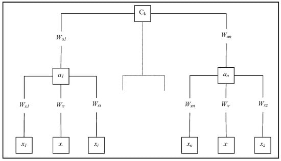
Figure 1.
The hierarchical structure of the model.
The hierarchical model can be variously structured using different levels of aggregation and intermediate criteria (aj) between the elementary characteristics (xi) and the aggregated indicators (ck).
The weight (wi) assigned to a characteristic or an aggregation of characteristics (an) is a scale factor which compares it with the others. (In a multi attribute model, the weights represent the trade-off between different parameters of evaluation. In particular, in the case of weighted-sum models, under the hypothesis of independency among preferences, weights can be considered as scale factors [10].) If the characteristic x1 weighs twice that of characteristic x2 in the aggregated criteria (a1), then the weight attributed to it should be twice the weight assigned to the second. Furthermore, passing from the worst to the best case in the first characteristic would have twice the importance of passing from the worst to the best state of the second characteristic. Therefore, the assignment of weights has to consider the possible states of each characteristic in a specific context [58].
To avoid the over/underestimation of weights assigned to a certain characteristic, a SWING procedure [59] was defined based on the priority (score) attributed at obtaining the maximum possible improvement in the characteristic under exam with respect to the maximum improvements obtainable in other characteristics. The bottom-up procedure is organized in five steps:
- For each node (an) of the hierarchy, the relative characteristics (xi) are identified
- For each characteristic, the best and the worst possible state is defined to obtain a set of maximum possible improvements on each characteristic.
- The characteristics (xi) are ordered according to the contribution in defining the complex variable represented by a node (an).
- Score are fixed out of 100, the score of the most important characteristics, with the remainders receiving a score according to their relative importance.
- Scores are normalized.
This procedure, described for the lower levels of the hierarchy, is repeated for the higher levels (i.e., aggregating an into ck).
The bottom-up approach was chosen as it first evaluated tangible characteristics, and then valuated the aggregations of synthetic indicators in the following step. This facilitated a self-learning process that improved the real estate expert’s familiarity and confidence with the weighting procedure. The outcome of the procedure were value functions that, given the characteristics (xi) of each real estate in a specific context, calculated the indicators ck.
The aggregation functions assume the following formulation:
where ck are the synthetic indicators; xi are the characteristics; wi are the weights of the i-th characteristics; and h are the nodes that separate in the hierarchical model the characteristic (xi) from the indicator ck (e.g., in the tree of Figure 1, there are two nodes).
3.1.3. The Model Estimation
The calibration of the model consists of the estimate of an econometric function which is able to transform the indicators (ck) into a market value (Vu). The complexity of the function transforming the indicators ck into market values strictly depends on the amount of market data available. With little data, nonparametric procedures should be adopted, whereas, if more data are available, multi-parametric techniques can be used. It must be noted that multi-parametric techniques allow for weights evaluation to move from the experts’ judgment towards econometric analysis. Thus, with more available market data, more aspects can be evaluated relying on the statistical analysis.
The hybrid valuation model (HVM), which combines these characteristics, can be expressed with the following formula:
where Vu is the value of the real estate (€ m−2); α and β are the estimated parameters with an econometric analysis; ck are the aggregated indicators; and xi are the characteristics of the single property.
Hence, the value increment of the real estate stock induced by an urban improvement is the following:
where Dj is the dimension of the j-th property (m2); Vujs is the value (€ m−2) of the j-th property without improvement; and Vujc is the value (€ m−2) of the j-th property with improvement.
The simulation has been realized in four phases:
- Identification of modified characteristics by eliminating high flooding (tides greater than 110 cm);
- Identification of the variation induced on the state of these variables;
- Calculus of the modified aggregated indicators (cl,p,t,e) using MAA models of Figures 3–6; and
- Calculus of the modified value using Equation (2).
Finally, the model was implemented in a GIS, based on maps representing the spatial distribution of the characteristics of properties and the property values, and was used for simulating the spatial distribution of real estate value changes induced by changes in characteristics.
3.2. A Hedonic-Multi Attribute Model for the Historic Center of Venice
The model for the valuation of urban improvements in Venice was based on a set of indicators (ck) synthetizing the characteristics of the real estate. The indicators were defined according to consolidated appraisal literature [57] that grouped the characteristics influencing the value in four categories:
- Location characteristics (cl), which includes environmental and urban quality like services, accessibility, infrastructure, amenities, pollution, noise, etc.;
- Position characteristics (cp), which describe the way the building is related to the surrounding context like views, brightness, etc.;
- Technical characteristics (ct), which comprehend architecture typology, finishing, maintenance, etc.; and
- Economic characteristics (ce), which regard those aspects that influence income, profitability, costs, etc.
The structure of each indicator and the weight assigned to the characteristics were assessed by an expert panel, comprising five of the most active real estate agents operating in Venice and following the steps illustrated in Figure 2. Figure 3, Figure 4, Figure 5 and Figure 6 report the structure of the aggregation function, its components and the weight assigned (in parenthesis) for each indicator (cl,p,t,e).
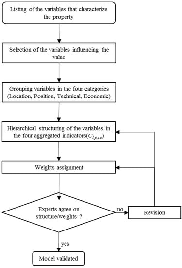
Figure 2.
The procedure eliciting the structure of the aggregate indicators.
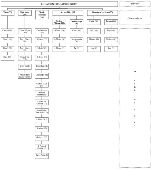
Figure 3.
The structure of the “location” indicator (cl).
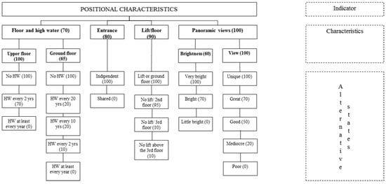
Figure 4.
The structure of the “position” indicator (cp).
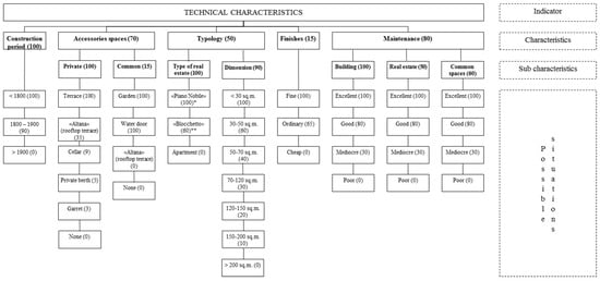
Figure 5.
The structure of the “technical” indicator (ct) (* “Piano Nobile” is a property, usually located on the first floor of Venetian palaces, with excellent finishes and decorations (frescoes) where the rich families of Venetian merchants lived in the past. ** “Blocchetto” is a popular Venetian property type consisting of two or more overlaid floors with independent access to public spaces: Calle or Campo).
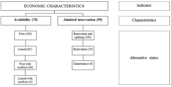
Figure 6.
The structure of the “economic” indicator (ce).
The econometric model was estimated using market data collected through a 2007 survey among real estate agencies in Venice (see Appendix A). The survey collected the prices and characteristics of 197 recently sold residential properties that were uniformly distributed throughout the Venice historic center. Table 1 and Table 2 provide a summary of the main characteristics of the sample.

Table 1.
Summary of cardinal variables of the sample.
Table 2.
Summary of nominal/ordinal variables of the sample.
Calibration was performed in the following phases:
- Calculation for each market data (comparable) of the aggregate indicators described above (cl,p,t,e);
- Stepwise OLS (ordinary least square) regression with the aggregate indicators as independent variables and the property prices (€ m−2) as dependent variables.
To consider the segmentation of the real estate market in Venice, two hedonic models were estimated. The first was based on properties purchased in primary touristic areas. The districts of primary touristic interest are Sestieri of S. Marco, the western zones of Castello, the eastern zones of Cannaregio, the Sestieri of Dorsoduro (central and eastern part) S. Croce, and S. Polo. The areas of prevailing local resident interest are the eastern areas of Castello, including S. Elena, the Giudecca Island with Sacca Fisola, S. Marta, and the western parts of Cannaregio (see Table 3 and Table 4). The second was estimated with reference to properties located in areas with relevant residential destination, or better, of minor touristic interest (see Table 5 and Table 6). To test the presence of heteroskedasticity, which is frequent when dealing with monetary dependent variables, the White and Breusch–Pagan tests were performed. Both tests rejected the null hypothesis of homoskedasticity in the subsample of the resident’s market segment and accepted it in the tourist’s segment subsample. Thus, to avoid distortions in standard error estimates, White’s “robust standard error” was adopted.
Table 3.
Pearson correlations test of the touristic sample (85 cases; Sig. 2-code in brackets).
Table 4.
The value function of touristic market segment, robust standard errors with respect to heteroskedasticity, HC1 variant.
Table 5.
Pearson correlations test of the resident samples (112 cases; Sig. 2-code in brackets).
Table 6.
The value function of residents’ market segment, robust standard errors with respect to heteroskedasticity, HC1 variant.
According to the OLS stepwise analysis, economic characteristics did not significantly influence the market price in the sample. Real estate values in the most attractive touristic areas were strongly influenced by location (district) and technical characteristics (finishes and state of repair). In the areas of prevalent local residential demand, a high and significant constant was observed. Where those wanting to live in Venice had a significant “base” they were willing to pay, to which the effects of the other characteristics were added. In these cases, positional and technical characteristics also appeared to be significant, but with different priorities. Technical characteristics had the highest coefficient, followed by position and location characteristics. For residents, the building characteristics appeared to be much more important than its location. Buyers seemed to be willing to sacrifice the prestige of a good location (higher presence of tourists) for good technical characteristics (maintenance and finishing); however, this was dependent on the high refurbishment costs and the conflicts between the resident’s life quality and tourist congestion.
3.3. The Geographic Model
The value functions developed in the previous paragraph were implemented in a GIS model to represent the spatial distribution of present property values and simulate changes induced by hypothetical urban improvements. In this study, GIS was used exclusively to represent the spatial distribution of features and values. No spatial statistical analysis was performed that could be an interesting development of the evaluation model. The GIS organized and geo-referenced the information to represent the state of each building in Venice in relation to the characteristics (xi) implemented in the valuation model. The layers adopted a raster grid of 1 m2 and were implemented using data collected for preparing the master plan for the historic center of Venice. Assuming the quality of the available information, some simplifications and elaborations were made. First, the available information referred to entire buildings rather than single flats, which are the most common property type purchased. For missing data, an interpolation between nearby points was necessary. Regarding the technical characteristics of the buildings, poor information was available to precisely define the state of indicator, so a uniform (most probable) state of repair was assumed for those buildings lacking specific information. The value functions applied to layers mapping the Venice property characteristics allowed us to map the aggregate indicators (cl and cp) and, finally, the real estate value. In the following paragraphs, some examples are illustrated.
3.3.1. The Distribution of Location Characteristics
The noise exposure of buildings noise exposure was assessed using the acoustic classification plan developed by the municipality of Venice. The document shows that noise was essentially due to boat traffic in the most important canals, and the presence of tourists and recreation facilities (mainly bars) in the most congested areas. Plan mapping provided a classification in zones with similar noise. Therefore, buildings in the various zones were assigned a relative noise class.
Flooding in Venice is an occurrence that happens as the result of a complex interplay of metrological and oceanographic phenomena. High tides are favored especially where strong winds from the south/south-east, such as the sirocco, blow for a long time. These winds push additional sea water into the lagoon through the three lagoon outlets, which add up to water flowing into the lagoon as a result of tidal flows and rising water levels flood Venice’s streets and squares. The phenomenon of high tides has been being systematically monitored in the municipality of Venice since the 1870s and allows for modeling frequencies of different flood levels.
The frequency of flooding was estimated with an interpolation between the level quotas given by the Municipality of Venice. The classification was made according to the frequency with which the areas flooded. According to the flood frequency, six classes were set, from the worst case of three or more floods per year, up to the best situation of less than one flooding in 100 years [60]. Figure 7 shows the annual distribution of tides higher than 110 cm for the period between 1872 and 2016.
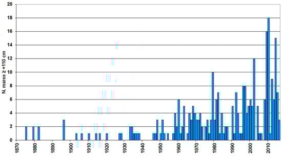
Figure 7.
Annual distribution of high tides (≥110 cm) recorded in Venice from 1872 to 2016 [60].
According to the experts’ judgments, properties in the historic center of Venice were first classified according to the six urban districts (Sestieri). This partition had to be further differentiated into 15. During the panel discussion, the touristic/residential vocation of the various areas of the center of Venice was also explored.
To qualify each building regarding its accessibility from public transport, a spatial-temporal relation was created assuming a speed of 4 km h−1 for pedestrians. Measuring the minimum distance from each building to the public boat stops along public walkways (using the network of canals as a barrier), a map of times needed to reach the nearest boat stop was created. This map was integrated with the travelling times of public transport from each boat stop towards the main access points to Venice from the mainland (the Piazzale Roma car park and S. Lucia railway station) at a speed of 7 km h−1. The result consisted of a layer of travel time from each building to the access point from the mainland.
The judgment on the density of services available was based on the linear distance towards public services (hospital and other sanitary services, schools and public administrations) in the historic center, and on the density of private services (using a classification of density of commercial services made by the local authority).
3.3.2. The Distribution of Position Characteristics
One of the positional characteristics that most characterizes the real estate in Venice is the frequency a building is flooded. This attribute is extremely important if the real estate is on the ground floor, while its importance decreases with the rising floor levels. Thus, for ground floors as well as for the upper floors, classification with reference to the level of exposure to high waters has been created.
Panorama quality was introduced into the geographic model to synthesize two factors: the building’s brightness and the view quality. Brightness was computed based on the minimum insolation of the buildings by assuming a value of 22° for the sun elevation, which corresponded (for the Venetian latitude) to an insolation at noon (azimuth 180°) during the months of December and January. The values obtained were then classified into three categories: little bright (values < 4), bright (values of 4–6), and very bright (values > 6).
Judgment on the view’s quality was related to the prestige of the urban areas that the building faces. The buildings facing S. Marco basin and squares (Piazza and Piazzetta) were classified as having a “unique” view; buildings facing the Grand Canal, major squares (Campi), and the main canals were computed as having a “prestigious view”; and buildings facing smaller canals and places was classified as having a “nice view”. The class “ordinary view” was attributed to the remaining buildings, except those with scarce brightness where the view was also assumed to be “scarce”.
The building period was based directly on the information gathered with a typological survey of the Venice municipality, which distinguished between pre-19th century, 19th century, and more recent buildings.
3.3.3. The Present Distribution of Residential Property Value
The distribution of real estate values was mapped by synthesizing the indicators described above. Data available did not offer enough information to allow the attribution of different judgments to single buildings for technical and economic characteristics. The synthesis considered that two different models were estimated for the areas of different tourist vocation. Therefore, it was necessary to consider that all areas of the historic center were attractive to tourists as well as for residents, but with different intensity. Hence, the spatial representation of the value of real estate was obtained by joining the model developed for the main touristic areas and the one for more “residential” districts. In other words:
where Vu is the real estate value (€ m−2); aT is the coefficient of tourist vocation; VuT is the real estate value (€ m−2) on the touristic market/location; and VuT is the real estate value (€ m−2) of the residential market/location. The coefficient of tourist vocation (e.g., S. Marco (1) and Sacca Fisola (0)) was obtained by interpolating expert judgments on homogenous areas where the center was subdivided.
4. The Simulation of Urban Improvements
The model illustrated in Section 5 was used to simulate the benefits (value gain) to the real estate produced by eliminating flooding of more than 110 cm due to the implementation of mobile barriers at outlets of the lagoon (MOSE). At present, the tidal level at which the gates will be raised is set at 110 cm, which aims to reduce the time the gates will be raised. Closing the gates limits access to the commercial harbors in Marghera, Chioggia, and the cruise ship harbor in Venice and is further expected to cause problems of water quality by interrupting the exchange of water between the lagoon and the sea. On the other hand, urban spaces need to be equipped for the range of tidal flooding not protected by the MOSE gates by raising the floor levels of public spaces [61,62]. As mentioned earlier the simulation was realized in four phases:
- Identification of modified characteristics by eliminating high flooding (tides greater than 110 cm);
- Identification of the variation induced on the state of these variables;
- Calculating the modified value using Equation (2).
The variation produced by the elimination of high tides essentially concerned the location and position of the properties. Therefore, the state of the following variables was modified:
- Location characteristics: The frequency of flooding was set to zero for areas situated above 110 cm above sea level, thus diminishing the flood frequency. For buildings situated in areas under 110 cm, the frequencies were reduced consequently.
- Position: Analogously, the frequency of building flooding was modified by eliminating those caused by tides higher than 110 cm above sea level.
The changes in the state of these variables produced a significant variation in the indicators cl and cp. After calculating the variations produced by the MOSE project in the indicators, the variation in residential value was calculated. Furthermore, the valuation was performed, for obvious reasons, separately for ground floors and for upper stories.
Results for the value increments on the ground floor (Figure 8) show a maximum value increase of 680 € m−2 that was registered in the areas most exposed to high waters. The average increase for ground floor dwellings was 340 € m−2, which corresponds to an average increase of 8.2%. A value increment for ground floor residential premises of approximately of 960 million € was obtained for the whole city.
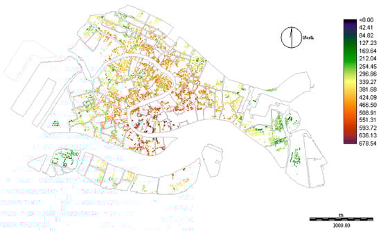
Figure 8.
Average value increments eliminating high water in ground floor residences (€ m−2).
Results for the value increments on the ground floor (Figure 9) show a maximum value increase of 580 € m−2 and the mean growth of real estate values for the upper floors was about 177 € m−2, which corresponded to an average increase of 3.8% and to a total increase for the upper floors of around 500 mln €. Comparison of the results for the value increments on the ground to those for upper floors shows that the value increase for upper floors was lower than those obtained for the ground floors, which can be attributed to the fact that upper floors suffer less from impacts of direct flooding although high levels of humidity due to saline intrusion into building elements require specific maintenance activities, too. The total increase for the ground and upper floors estimated is about 1.4 billion €. Table 7 shows average value increments for each Sestiere considered and Figure 10 shows the total average increases. Interestingly, it can be noted that there is also a significant value increase for buildings not directly exposed to the risk of flood. This improvement is due to two aspects: first, improvements in accessibility, as flooding significantly impedes people’s mobility; and, second, because the real estate market appreciates the reduction in humidity and salinity damage to the buildings. This corresponds to decreasing maintenance costs, which are usually very high in Venice.
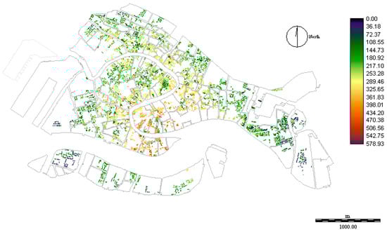
Figure 9.
Average value increments of eliminating high water for upper stories.
Table 7.
Average value increments for the Sestiere (€ m−2).

Figure 10.
Average value increases (€ m−2).
Value increments were higher in the Sestieri of S. Polo, S. Marco, S. Croce, and Dorsoduro, whereas minor increments were registered in Castello and Giudecca due to lower real estate value.
5. Conclusions
The economic evaluation of urban improvements is a focal point in urban planning and the decision-making process when regarding public investment. However, they are not widely used by public decision makers due to the difficulty and burden of assessments. This paper presented a method to evaluate the impact on real estate values of urban improvements using a hybrid hedonic multi attribute model, integrated into a GIS. The model adopted a multi attribute procedure to calculate a set of aggregate indicators derived from expert opinions and a hedonic function to transform them into market values. The model was used to simulate the impacts of the realization of flood protection measures (the MOSE project) on housing values in the historic center of Venice.
Despite the experimental application of the model, some interesting results were obtained. First, it proposed a procedure for synthesizing information from market transactions with the know-how of real estate operators. This allows the use heterogeneous sources of information on preferences of the real estate market available and organizes it in a flexible and transparent way. Second, the hierarchical structuring of the valuation model allowed the thorough analysis of the determinants of real estate value, evidencing the role of each characteristics. Third, the implementation of the model in a GIS increased its flexibility and widened the utility of the obtained results. The possibility of mapping the real estate characteristics and values allow for the verification of their coherence and widens the possibility of application. Furthermore, the experimental application permitted a first evaluation of its concrete applicability, and the results, despite the numerous simplifications, appear to be plausible and robust, especially considering the transparent and logical process from which they were obtained.
This suggests that using the model not only for una tantum evaluations, but also for permanent mass appraisal services, addresses different measures of urban improvements. The model, especially if implemented in a permanent evaluation service, lends itself to many uses, particularly: (a) the ex-ante cost–benefit analysis of public investments; (b) the evaluation of impact and distribution of costs and benefits of planning; (c) the assessment of value for the determination of property local taxes; and (d) an information system for real estate valuation.
The experimental evaluation of the MOSE project showed that the elimination of flooding caused by higher tides produced a significant increase in real estate values in Venice. This improvement was higher on ground floor properties (+8.2%) than in upper floor real estate (+3.8%). Considering both upper and ground floors the increase in real estate values is about 5.9%. The overall residential real estate value improvements resulting from the simulation was approximately 1.4 billion € (213 € m−2). As mentioned in Section 2, it is difficult to compare the results of this study with those reported in literature, because the phenomena considered are different. In this study, flooding is a phenomenon that happens more times a year and does not involve destructive effects, with which the city lives for centuries through adaptation measure, such as the raising of the shores. Instead, in the previous literature, the phenomena analyzed involve destructive effect, with generally a 100-years return period. Having regard to the foregoing, the total increase in real estate, deriving from this study, equal 5.9%, which is similar to the estimations of the hedonic evaluation reported in the literature, showing a varying effect deriving from the exposition to flood hazard, with the higher frequency around 5–7%.
The valuation presented here has some limitations. First, it was developed to illustrate the application of the model and the quality of the results suffers from the scarcity of market data. Second, it presents static assessments that did not consider the effect of property use changes caused by drastic reductions in flood frequency. Third, it assumed that the present value was not affected by the expectations of the MOSE project. Finally, it also assumed the current flood frequency and did not consider the possible effects of the sea level rise caused by climate change, which might lead to complex impacts under frequent closures of MOSE flood gates These limitations in the application of the model suggest some undervaluation of the effects of the MOSE project on the real estate value of Venice. Other potentially interesting applications of the model could regard, for instance changes in the pattern of access to the city, which is actually concentrated on two main points (railway station and parking site in Piazzale Roma) while a more diffuse organization of arrivals in the city could contribute to change preferences also of the real estate market.
In conclusion, the procedure illustrated has a large margin for improvement, especially with good data quantity and quality, and a more intensive interaction with real estate experts. A higher quality of data might provide the opportunity to apply econometric valuations to more detailed indicators, thus, moving the valuations from expert judgment to rigorous statistical analysis. On the other hand, the possibility to deepen collaboration with experts might improve the formalization of expertise using more sophisticated and precise procedures [34].
Acknowledgments
The research was funded by FEEM (Fondazione Eni Enrico Mattei). The authors would like to thank the anonymous reviewers for their helpful and constructive comments that contributed to improving the final version of the paper.
Author Contributions
P.R. performed Section 1, Section 3.1, Section 4 and Section 5; M.B. built up Section 1, Section 2, Section 3.2, Section 3.3, Section 4 and Section 5; C.G. developed Section 1, Section 3.3 and Section 5; R.B. implemented Section 1, Section 2, Section 3.2 and Section 5.
Conflicts of Interest
The authors declare no conflict of interest.
Appendix A.
Table A1.
Scheme for data collection.
Table A1.
Scheme for data collection.
| Property _________ | |||
| Date of purchase (month/year) | |||
| Price (€) | |||
| Floor area (m2) | |||
| Location (house number or position on the map) | |||
| Positional Characteristics | |||
| 1. | Flooding with high water | Tide level at which the ground floor of building is flooded (cm) | |
| Flooding frequency per year (average) | |||
| 2. | Entrance/Lift | Independent entrance | |
| Is there a lift serving the property? | |||
| 3. | Construction period | Before 1800 | |
| 1800–1900 | |||
| 1900–1945 | |||
| After 1945 | |||
| 4. | Brightness of the property | Very bright | |
| Bright | |||
| Little bright | |||
| Quality of the view from the property | Unique | ||
| Great | |||
| Good | |||
| Mediocre | |||
| Poor | |||
| 5. | Accessory | Terrace | |
| “Altana” | |||
| Cellar | |||
| Private berth | |||
| Garret | |||
| Technical Characteristics | |||
| 1. | Dimension | <30 m2 | |
| 30–50 m2 | |||
| 50–70 m2 | |||
| 70–120 m2 | |||
| 120–150 m2 | |||
| 150–200 m2 | |||
| 2. | Typology | “Piano Nobile” | |
| “Blocchetto” | |||
| Apartment | |||
| 3. | Finishes | Fine | |
| Ordinary | |||
| Cheap | |||
| 4. | Building maintenance | Excellent | |
| Good | |||
| Mediocre | |||
| Poor | |||
| Real estate maintenance | Excellent | ||
| Good | |||
| Mediocre | |||
| Poor | |||
| Common spaces maintenance | Excellent | ||
| Good | |||
| Mediocre | |||
| Poor | |||
| 5. | Floor | GF, 1st, 2nd, 3rd, 4th or 5th floor | |
| Economic Characteristics | |||
| 1. | Availability | Free | |
| Rented | |||
| Free with usufruct | |||
| Rented with usufruct | |||
References
- Hanley, N.; Knight, J. Valuing the environment: Recent UK experience and an application to Green Belt Land. J. Environ. Plan. Manag. 1992, 35, 145–160. [Google Scholar] [CrossRef]
- Bullock, C.H. Valuing Urban Green Space: Hypothetical Alternatives and the Status Quo. J. Environ. Plan. Manag. 2008, 51, 15–35. [Google Scholar] [CrossRef]
- Whitehead, J.C.; Haab, T.C.; Huang, J.-C. Measuring recreation benefits of quality improvements with revealed and stated behavior data. Resour. Energy Econ. 2000, 22, 339–354. [Google Scholar] [CrossRef]
- Pearce, D.; Atkinson, G.; Mourato, S. Cost-Benefit Analysis and the Environment: Recent Developments; Organisation for Economic Co-Operation and Development: Paris, France, 2006; ISBN 978-92-64-01004-8. [Google Scholar]
- Crompton, J.L. The impact of parks on property values. empirical evidence from the past two decades in the United States. Manag. Leisure 2005, 10, 203–218. [Google Scholar] [CrossRef]
- Cloudburst Management Pays Off 2014—Climate-ADAPT. Available online: http://climate-adapt.eea.europa.eu/repository/11286781.pdf/view (accessed on 16 October 2017).
- Bender, A.; Din, A.; Favarger, P.; Hoesli, M.; Laakso, J. An analysis of perceptions concerning the environmental quality of housing in Geneva. Urban Stud. 1997, 34, 503–513. [Google Scholar] [CrossRef]
- Din, A.; Hoesli, M.; Bender, A. Environmental variables and real estate prices. Urban Stud. 2001, 38, 1989–2000. [Google Scholar] [CrossRef]
- Baranzini, A.; Ramirez, J.V. Paying for quietness: The impact of noise on Geneva rents. Urban Stud. 2005, 42, 633–646. [Google Scholar] [CrossRef]
- Lake, I.R.; Lovett, A.A.; Bateman, I.J.; Langford, I.H. Modelling environmental influences on property prices in an urban environment. Comput. Environ. Urban Syst. 1998, 22, 121–136. [Google Scholar] [CrossRef]
- Del Giudice, V.; De Paola, P. The Effects of Noise Pollution Produced by Road Traffic of Naples Beltway on Residential Real Estate Values; Trans Tech Publications: Zürich, Switzerland, 2014; Volume 587, pp. 2176–2182. [Google Scholar]
- Del Giudice, V.; De Paola, P.; Manganelli, B.; Forte, F. The monetary valuation of environmental externalities through the analysis of real estate prices. Sustainability 2017, 9, 229. [Google Scholar] [CrossRef]
- Gao, X.; Asami, Y. The external effects of local attributes on living environment in detached residential blocks in Tokyo. Urban Stud. 2001, 38, 487–505. [Google Scholar] [CrossRef]
- Zabel, J.E.; Kiel, K.A. Estimating the demand for air quality in four US cities. Land Econ. 2000, 76, 174–194. [Google Scholar] [CrossRef]
- Irwin, E.G. The effects of open space on residential property values. Land Econ. 2002, 78, 465–480. [Google Scholar] [CrossRef]
- Kim, C.W.; Phipps, T.T.; Anselin, L. Measuring the benefits of air quality improvement: A spatial hedonic approach. J. Environ. Econ. Manag. 2003, 45, 24–39. [Google Scholar] [CrossRef]
- Crane, R.; Daniere, A.; Harwood, S. The contribution of environmental amenities to low-income housing: A comparative study of Bangkok and Jakarta. Urban Stud. 1997, 34, 1495–1512. [Google Scholar] [CrossRef]
- Coulson, N.E.; Leichenko, R.M. The internal and external impact of historical designation on property values. J. Real Estate Financ. Econ. 2001, 23, 113–124. [Google Scholar] [CrossRef]
- Votsis, A. Planning for green infrastructure: The spatial effects of parks, forests, and fields on Helsinki’s apartment prices. Ecol. Econ. 2017, 132, 279–289. [Google Scholar] [CrossRef]
- Bond, M.T.; Seiler, V.L.; Seiler, M.J. Residential real estate prices: A room with a view. J. Real Estate Res. 2002, 23, 129–138. [Google Scholar]
- Tajani, F.; Morano, P.; Locurcio, M.; Torre, C.M. Data-driven techniques for mass appraisals. Applications to the residential market of the city of Bari (Italy). Int. J. Bus. Intell. Data Min. 2016, 11, 109–129. [Google Scholar] [CrossRef]
- Walsh, P.; Griffiths, C.; Guignet, D.; Klemick, H. Modeling the Property Price Impact of Water Quality in 14 Chesapeake Bay Counties. Ecol. Econ. 2017, 135, 103–113. [Google Scholar] [CrossRef]
- Tomkins, J.; Topham, N.; Twomey, J.; Ward, R. Noise versus access: The impact of an airport in an urban property market. Urban Stud. 1998, 35, 243–258. [Google Scholar] [CrossRef]
- Mei, Y.; Hite, D.; Sohngen, B. Demand for urban tree cover: A two-stage hedonic price analysis in California. For. Policy Econ. 2017, 83, 29–35. [Google Scholar] [CrossRef]
- Saginor, J.; Ge, Y. Do hurricanes matter?: A case study of the residential real estate market in Brunswick County, North Carolina. Int. J. Hous. Mark. Anal. 2017, 10, 352–370. [Google Scholar] [CrossRef]
- Chay, K.Y.; Greenstone, M. Does air quality matter? Evidence from the housing market. J. Polit. Econ. 2005, 113, 376–424. [Google Scholar] [CrossRef]
- Paterson, R.W.; Boyle, K.J. Out of sight, out of mind? Using GIS to incorporate visibility in hedonic property value models. Land Econ. 2002, 78, 417–425. [Google Scholar] [CrossRef]
- Wu, J.; Adams, R.M.; Plantinga, A.J. Amenities in an urban equilibrium model: Residential development in Portland, Oregon. Land Econ. 2004, 80, 19–32. [Google Scholar] [CrossRef]
- Anselin, L.; Lozano-Gracia, N.; Deichmann, U.; Lall, S. Valuing Access to Water-A Spatial Hedonic Approach, with an Application to Bangalore, India. Spat. Econ. Anal. 2010, 5, 161–179. [Google Scholar] [CrossRef]
- Curto, R.; Fregonara, E.; Semeraro, P. A spatial analysis for the real estate market applications. In Advances in Automated Valuation Modeling; Springer: Cham, Switzerland, 2017; pp. 163–179. [Google Scholar]
- Fotheringham, A.S.; Brunsdon, C.; Charlton, M. Geographically Weighted Regression: The Analysis of Spatially Varying Relationships; John Wiley & Sons: Chichester, UK, 2003; ISBN 0-470-85525-8. [Google Scholar]
- Herath, S.; Choumert, J.; Maier, G. The value of the greenbelt in Vienna: A spatial hedonic analysis. Ann. Reg. Sci. 2015, 54, 349–374. [Google Scholar] [CrossRef]
- Bin, O.; Poulter, B.; Dumas, C.F.; Whitehead, J.C. Measuring the Impact of Sea-Level Rise on Coastal Real Estate: A Hedonic Property Model Approach. J. Reg. Sci. 2011, 51, 751–767. [Google Scholar] [CrossRef]
- Orford, S.; Dorling, D.; Harris, R. Review of Visualisation in the Social Sciences: A State of the Art Survey and Report; Advisory Group on Computer Graphics: Bristol, UK, 1998. [Google Scholar]
- Roebeling, P.; Saraiva, M.; Palla, A.; Gnecco, I.; Teotónio, C.; Fidelis, T.; Martins, F.; Alves, H.; Rocha, J. Assessing the socio-economic impacts of green/blue space, urban residential and road infrastructure projects in the Confluence (Lyon): A hedonic pricing simulation approach. J. Environ. Plan. Manag. 2017, 60, 482–499. [Google Scholar] [CrossRef]
- Wen, H.-Z.; Jia, S.-H.; Guo, X.-Y. Hedonic price analysis of urban housing: An empirical research on Hangzhou, China. J. Zhejiang Univ. 2005, 6, 907–914. [Google Scholar] [CrossRef]
- Donnelly, W.A. Hedonic Price Analysis of the Effect of a Floodplain on Property Values. J. Am. Water Resour. Assoc. 1989, 25, 581–586. [Google Scholar] [CrossRef]
- Harrison, D.T.; Smersh, G.; Schwartz, A. Environmental determinants of housing prices: The impact of flood zone status. J. Real Estate Res. 2001, 21, 3–20. [Google Scholar]
- Bin, O.; Polasky, S. Effects of flood hazards on property values: Evidence before and after Hurricane Floyd. Land Econ. 2004, 80, 490–500. [Google Scholar] [CrossRef]
- Bin, O.; Kruse, J.B. Real estate market response to coastal flood hazards. Nat. Hazards Rev. 2006, 7, 137–144. [Google Scholar] [CrossRef]
- Bin, O.; Kruse, J.B.; Landry, C.E. Flood hazards, insurance rates, and amenities: Evidence from the coastal housing market. J. Risk Insur. 2008, 75, 63–82. [Google Scholar] [CrossRef]
- Daniel, V.E.; Florax, R.J.; Rietveld, P. Flooding risk and housing values: An economic assessment of environmental hazard. Ecol. Econ. 2009, 69, 355–365. [Google Scholar] [CrossRef]
- Samarasinghe, O.; Sharp, B. Flood prone risk and amenity values: A spatial hedonic analysis. Aust. J. Agric. Resour. Econ. 2010, 54, 457–475. [Google Scholar] [CrossRef]
- McKenzie, R.; Levendis, J. Flood Hazards and Urban Housing Markets: The Effects of Katrina on New Orleans. J. Real Estate Financ. Econ. 2010, 40, 62–76. [Google Scholar] [CrossRef]
- Bin, O.; Landry, C.E.; Meyer, G.F. Riparian buffers and hedonic prices: A quasi-experimental analysis of residential property values in the Neuse River basin. Am. J. Agric. Econ. 2009, 91, 1067–1079. [Google Scholar] [CrossRef]
- Rambaldi, A.N.; Fletcher, C.S.; Collins, K.; McAllister, R.R. Housing shadow prices in an inundation-prone suburb. Urban Stud. 2013, 50, 1889–1905. [Google Scholar] [CrossRef]
- Bin, O.; Landry, C.E. Changes in implicit flood risk premiums: Empirical evidence from the housing market. J. Environ. Econ. Manag. 2013, 65, 361–376. [Google Scholar] [CrossRef]
- Fu, X.; Song, J.; Sun, B.; Peng, Z.-R. “Living on the edge”: Estimating the economic cost of sea level rise on coastal real estate in the Tampa Bay region, Florida. Ocean Coast. Manag. 2016, 133, 11–17. [Google Scholar] [CrossRef]
- Rosen, S. Hedonic prices and implicit markets: Product differentiation in pure competition. J. Polit. Econ. 1974, 82, 34–55. [Google Scholar] [CrossRef]
- Freeman, A.M., III. Hedonic prices, property values and measuring environmental benefits: A survey of the issues. In Measurement in Public Choice; Springer: London, UK, 1981; pp. 13–32. [Google Scholar]
- Witte, A.D.; Sumka, H.J.; Erekson, H. An estimate of a structural hedonic price model of the housing market: An application of Rosen’s theory of implicit markets. Econom. J. Econom. Soc. 1979, 1151–1173. [Google Scholar] [CrossRef]
- Diamond, D.B.; Smith, B.A. Simultaneity in the market for housing characteristics. J. Urban Econ. 1985, 17, 280–292. [Google Scholar] [CrossRef]
- Curto, R. Mercato delle abitazioni e valori: Il caso di Torino. Genio Rurale 1990, 5, 11–27. [Google Scholar]
- Ozanne, L.; Malpezzi, S. The efficacy of hedonic estimation with the annual housing survey. Evidence from the demand experiment. J. Econ. Soc. Meas. 1985, 13, 153–172. [Google Scholar]
- Curto, R. L’uso Delle Tecniche Multicriteri Come Procedimenti Pluriparametrici; CELID: Torino, Italy, 2005. [Google Scholar]
- Rosato, P.; Lisini, L. I metodi di analisi quantitativa nell’estimo immobiliare: Una valutazione comparata. In Estimo E Valutazione Metodol. E Casi Studio; DEI Tipogr. Genio Civ.: Roma, Italy, 2007; pp. 45–60. [Google Scholar]
- Forte, C.; De’Rossi, B.; Ruffolo, G. Principi di Economia ed Estimo; Etas Libri: Milano, Italy, 1974. [Google Scholar]
- Belton, V.; Stewart, T. Multiple Criteria Decision Analysis: An Integrated Approach; Springer Science & Business Media: Berlin/Heidelberg, Germany, 2002; ISBN 0-7923-7505-X. [Google Scholar]
- Von Winterfeldt, D.; Edwards, W. Decision Analysis and Behavioral Research; Cambridge University Press: Cambridge, UK, 1993. [Google Scholar]
- Comune di Venezia Distribuzione Annuale Alte e Basse Maree. Available online: http://www.comune.venezia.it/it/content/distribuzione-annuale-delle-alte-maree-110-cm (accessed on 26 November 2017).
- Umgiesser, G.; Matticchio, B. Simulating the mobile barrier (MOSE) operation in the Venice Lagoon, Italy: Global sea level rise and its implication for navigation. Ocean Dyn. 2006, 56, 320–332. [Google Scholar] [CrossRef]
- Vergano, L.; Umgiesser, G.; Nunes, P.A. An economic assessment of the impacts of the MOSE barriers on Venice port activities. Transp. Res. Part D Transp. Environ. 2010, 15, 343–349. [Google Scholar] [CrossRef]
© 2017 by the authors. Licensee MDPI, Basel, Switzerland. This article is an open access article distributed under the terms and conditions of the Creative Commons Attribution (CC BY) license (http://creativecommons.org/licenses/by/4.0/).