Urban and Rural—Population and Energy Consumption Dynamics in Local Authorities within England and Wales

Abstract

The formulation of feasible and pragmatic policies that mitigate climate change would require a thorough understanding of the interconnectivity that exists between environment, energy, and the composition of our settlements both urban and rural. This study explores the patterns of energy consumption in England and Wales by investigating consumption behavior within domestic and transport sectors as a function of city characteristics, such as population, density, and density distribution for 346 Local Authority Units (LAU). Patterns observed linking energetic behavior of these LAUs to their respective population and area characteristics highlight some distinctly contrasting consumption behaviors within urban and rural zones. This provides an overview of the correlation between urban/rural status, population, and energy consumption and highlights points of interest for further research and policy intervention. The findings show that energy consumption across cities follows common power law scaling increasing sub-linearly with their population regardless of their urban/rural classification. However, when considering per capita and sector specific consumptions, decreasing per capita consumption patterns are observed for growing population densities within more uniformly populated urban LAUs. This is while rural and sparsely populated LAUs exhibit sharply different patterns for gas, electricity, and transport per capita consumption.

1. Introduction

The year 2009 saw a subtle and yet fundamentally significant change of the world. United Nation Population Division [1] reported that, by midyear 2009, the total number of people living in urban and metropolitan areas across the world exceeded that of those still inhabiting rural areas. While 3.3 billion at the time, the urban population, and by extension the spatial development associated with it, is projected to soar to almost 5 billion people by 2030 with over 80% of this growth taking place in developing regions. This growth, inevitable in nature, can be identified as a response to the far more favorable environments urban settings potentially offer in terms of job opportunities, education, and most other services [2].

Human settlements have been identified to be responsible for approximately 76% of the total global energy consumption corresponding to a conspicuous 60% of today’s total global fossil fuel consumption [3] and 71% of the direct energy-related CO₂ emissions [4]. The importance and significance of their contribution towards climate change and the necessary policies to address this has slowly become more widely acknowledged.

As such, a crucial role in any municipal planning process is the formulation of practical and feasible strategies to mitigate for and achieve environmental targets. Subsequently, associated issues arising include balancing different scale renewable technologies and energy efficiency measures across countries, cities, and buildings, addressing the need for energy storage and the suitable scale for them, and finally, the engineering understanding of their collective implications [5]. Formulation of practical and feasible strategies to mitigate climate change on either an urban or a rural scale and achieve environmental targets would require a much better apprehension of the interconnectivity that exists between the urban form, environment, and energy and the dynamics informing energy consumption. Yet, there has been and remains a lack of adequate understanding and clarity surrounding the drivers of the energy consumption and environmental emissions within cities [6,7,8]. This requires a fundamental understanding of the potential interconnectivity that exists between urban form and its inhabitants, the environment, consumption patterns, and the ways in which these could be exploited to plan and design for more sustainable and energy efficient cities and settlements.

Studies delving into the energy metabolism of urban environments and cities have revealed a few intriguing trends between energy variations across cities and their composition. For instance, in the late 80s and early 90s, Newman and Kenworthy [9,10] studied the energy consumption of transportation systems within cities. As part of the study, the variations of the transport energy use were investigated against population density of several major urban zones noting the annual consumption of fuel for transport is inversely proportional to population density in a power law. Also on a neighborhood scale, in a case study performed on low- and high-density areas in Toronto, Norman et al. [11] note a lower per person energy associated with the high-density development in transportation, building operations, and material sectors. Similarly, O’Brien et al. [12] suggest an overall decreasing behavior for the net energy use in cities, consisting mainly of household and transportation uses, with increasing housing density. A study of Australian households [13] provides analogous findings suggesting that despite urban households being responsible for higher energy consumptions when considering their larger consumption of goods and services, lower direct energy use levels, i.e., electricity, fuel, etc., are related to the households in the urban areas as opposed to those within the suburban and rural regions. Studies of this nature, which often indicate that increasing population/built density is correlated with decreasing urban energy consumption profiles, are mostly rooted in and can be explained by a theoretical expectation regarding consumption and accessibility within denser areas. A theoretical modelling of energy demand for different urban morphologies based on four case study cities of London, Paris, Berlin, and Istanbul confirms this by finding potential for significant savings achievable in heat-demand through higher built densities [14]. Hui [15] cites four reasons as to why high density built-environment and cities are expected to be more efficient in their energy use: (i) the compactness and higher densities results in lower consumptions within the buildings; (ii) the reduced time of travel and communication characteristics are advantageous towards better transportation performance; (iii) the implementation of novel and emerging technologies is more easily achieved; and (iv) the wider options and possibility of mixing land use would contribute towards higher efficiencies.

Thermodynamic principles could often be expected to suggest a decreasing overall consumption pattern in dwellings against increasing population density. Taking increasing population density to indicate denser construction forms [16], the more compactly built forms tend to provide smaller surface-to-volume ratios and hence lower potential environmental losses and overall urban consumption. Jones and Kammen [17], however, in their study of a large number of urban and suburban areas in the US and their household carbon and energy footprint, note the role of the quality of construction and the current state of the building stock, specifically within core urban areas, as sources of departure from these expected norms. In a similar manner, Minx et al. [18] analyze the carbon footprint of human settlements in the UK at a high spatial granularity noting a limited influence of the density on emissions contrasted with a stronger correlation of the CO₂ emissions with the socio-economic drivers. They also report generally higher levels of per capita emission associated with urban areas. Looking at CO₂ emissions in the UK on an even finer resolution, Baiocchi et al. [19] reject the adequacy of “one-size-fit-all” general models and use a tree regression model to establish different settlement types with similar emission patterns based on a mix of indicators, namely, density, income, household size, heating degrees-day, number of houses in poor conditions, and access to centralized heating technologies.

In a decidedly different approach to cities, through a series of analyses based on large urban datasets pertaining to the United States, China, and Europe, Bettencourt and West [20] and Bettencourt et al. [21], put forward the notion of “universal features” with special emphasis put on size of the city, mostly expressed and represented as the total population of inhabitants, as the primary determinant of urban characteristics with its geography, design, and history to follow. Their observation notes that cities’ properties averaged at a macroscale, e.g., number of patents, crimes reported, GDP, etc., scales with their population through simple power laws in a range of sub- to super-linear relations [22,23]. The availability of free and publicly accessible data on a range of city indicators has since provided opportunities to investigate the existence of similar scaling behaviors across different countries and for various other indicators including but not limited to the area of the city [24,25,26], length and area of infrastructure (e.g., length of road networks [27,28,29,30], electricity cables [21], etc.), and CO₂ emissions and energy dissipation [16,28,31,32]. These studies also make the observation that certain properties consistently exhibit specific scaling regimes with metrics describing built infrastructure showing sub-linear scaling, demonstrative of increasing efficiencies in larger cities, and those descriptive of individual interactions and processes, i.e., wealth, information, etc., displaying super-linear scaling. However, the universality of these exponents and their sensitivity to the choice of settlement boundary has recently been pointed out [33,34], especially in scaling patterns relating to energy and CO₂ emissions where different studies report exponents with broad or conflicting interval ranges.

The following explores the existence of similar power law relations linking the domestic and transport consumption with population and population density at a local authority level in a UK context and investigates whether and how the degree of urbanization of these administrative units impacts the dynamics of consumption with respect to population and what implications may arise as a result of these differences between urban and rural local authority units (LAU).

2. Data and Methods

The study presented in this work incorporates population data gathered through the UK 2011 census [35], and sub-national energy consumption statistics made available by the Department of Energy & Climate Change (DECC) for the same year [36] to perform the exploratory analysis. The census data reported for local authorities through the Office for National Statistics (ONS) has been accessed on a higher resolution scale through the middle-layer super output areas (MSOA), defined by the ONS as set up by zone-design software complying with social homogeneity constraints with a typical average population of 7200 residents or just over 1900 households fitted within the boundaries of local authorities [37]. The consumption data from DECC, however, has directly been used in the aggregated form at the local authority level. For domestic electricity and gas, the data is prepared by DECC based on an aggregation of consumption data of individual meters assigned domestic or otherwise based on cutoff values and data pertaining to postcode classifications. The road transport fuel data are, however, modeled by Ricardo Energy & Environment [38] on behalf of DECC and utilize estimates of vehicle fleet composition, fuel consumption factors for different fleets, and surveys of traffic flow on different road types, see DECC methodology guidebook for further details pertaining to all three datasets [39].

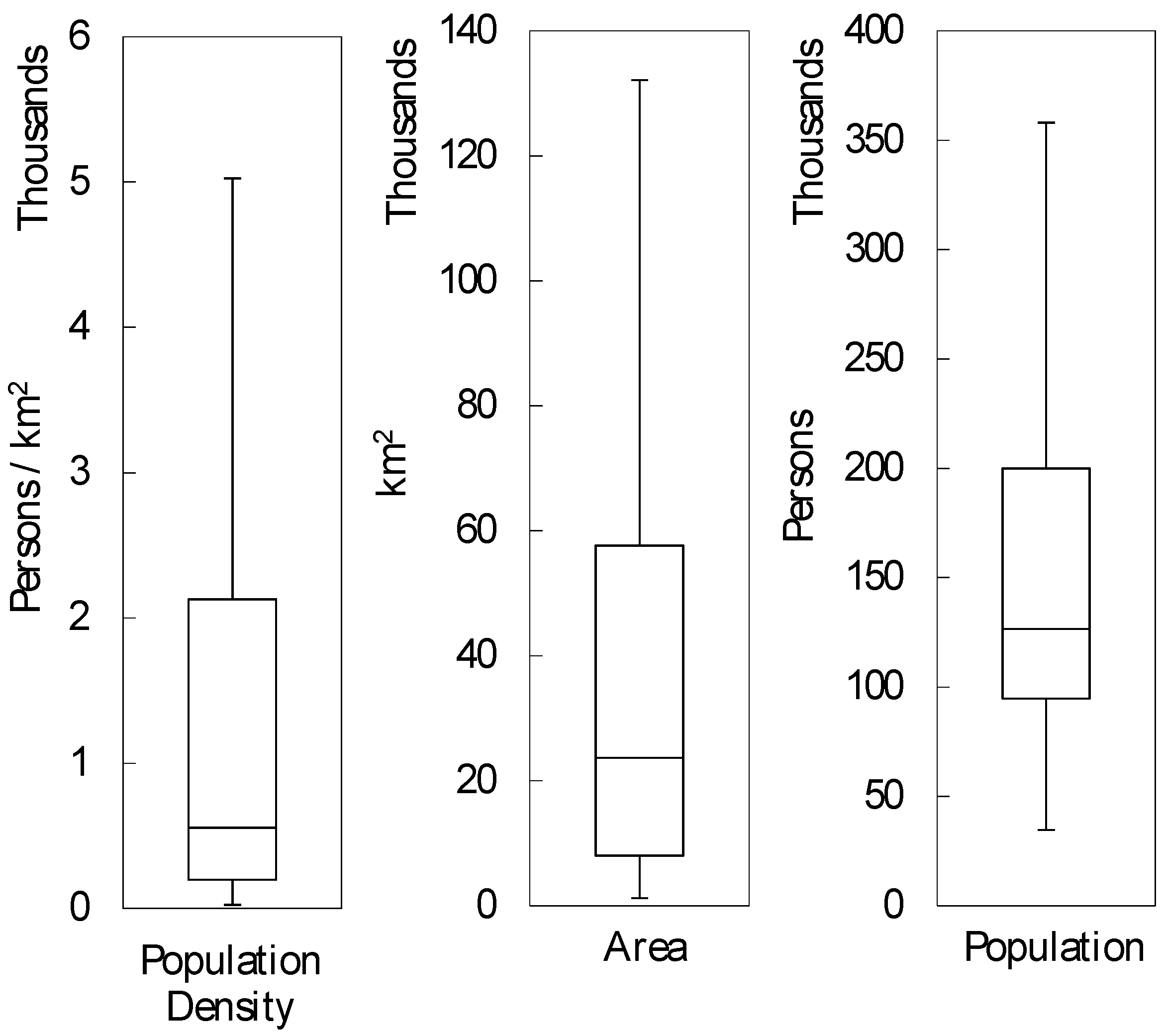
For the UK, local authorities constitute an administrative point in the local government and are treated as cities or city regions for the purposes of this study. Although there are a total of 326 authorities in England and 22 in Wales [37], due to the focus on domestic consumption and road transport here, the local authorities of City of London and Isles of Scilly have been excluded because of a mix of unique corporate function and exceptionally low total resident population respectively, hence outlier behavior in terms of population and consumption characteristics. See Figure 1 for a summary of the data retrieved for the remaining 346 local authorities.

The Department for Environment, Food & Rural Affairs (DEFRA) provides a six-tier category for urban/rural classification of local authorities [40] based on cutoff population counts and determining the total portion of urban or rural population in each local authority with some considerations for the “geographic design of local authority areas”. Here, on the other hand, a Gini coefficient indicator, calculated for each LAU based on the population density in all MSOAs building up that local authority is used according to

$$G_{LAU}=\frac{{\sum }_i^N{\sum }_j^N\left|y_i-y_j\right|}{2N^2\overline{y}}$$

(1)

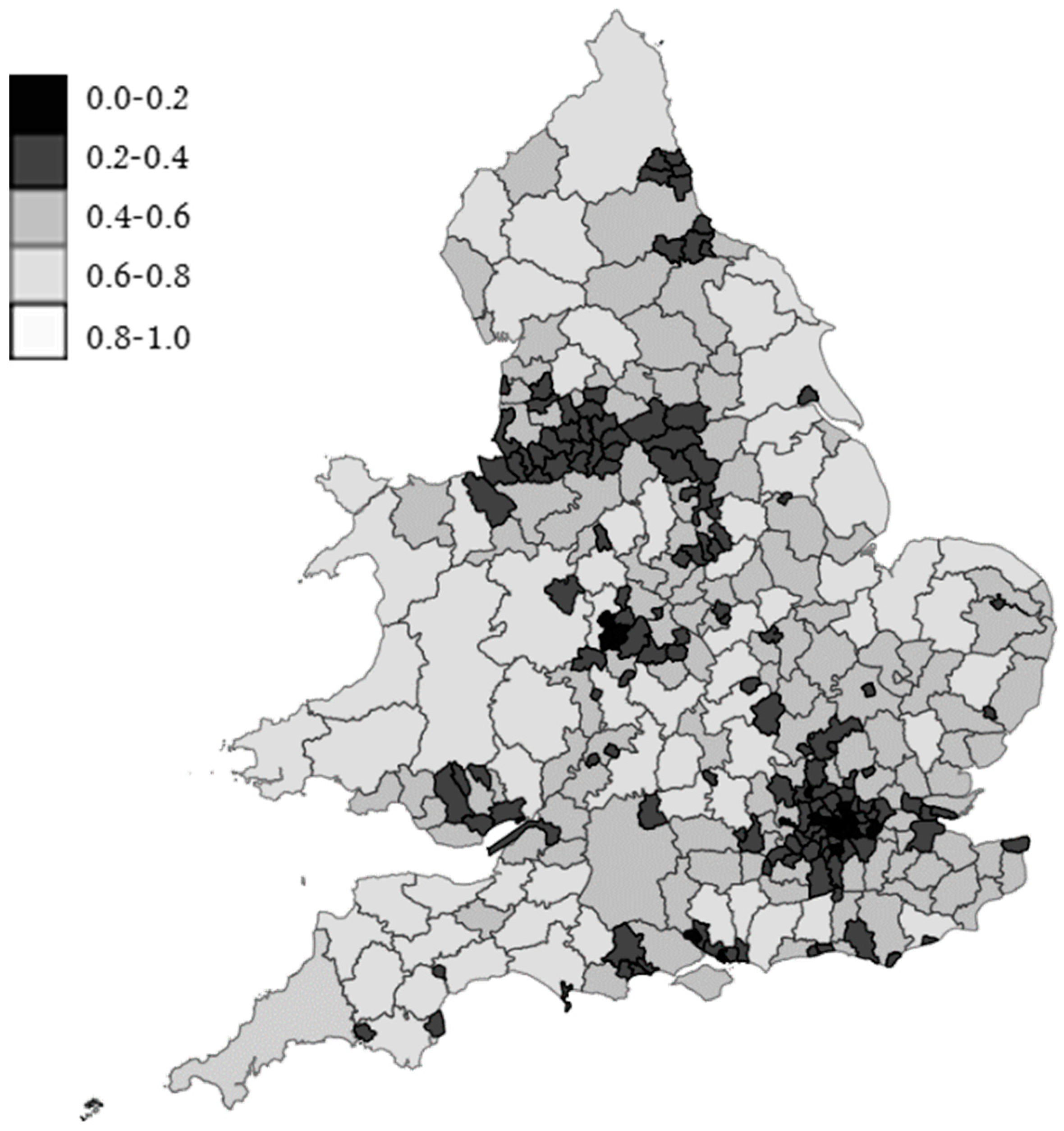
where $N$ and $y$ are the number and population density of MSOAs respectively and $\overline{y}$ denotes average population density of all comprising MSOAs for each LAU [41,42]. The index provides a measure of inequality of population density across the MSOAs of each authority unit. Values closer to 0 are indicative of a more uniform distribution of population over the area of the LAU whereas those closer to unity point to an extreme disparity between the population density of different MSOAs in the same LAU. As such, it is expected that rural authorities that have only a handful of MSOAs where the settlements are located with larger densities and numerous MSOAs enveloping unpopulated and empty land would exhibit larger Gini coefficients compared with their urban counterparts which are not expected to have sparsely populated MSOAs, see Figure 2. Consequently, the choice of the Gini coefficient based on population density of constituting MSAOs also enables an assessment of the dispersion and homogeneity of population distribution within each LAU and therefore was preferred over the DEFRA’s categorical classification [41]. For the urban/rural classification presented here, a cutoff value of 0.4 has been utilized with those below the unit marked as urban and the rest rural. It should be noted that the method utilized here matches that of DEFRA for a majority of the local authorities (identifying 161 urban LAUs as opposed to the 181 within the first three urban tiers of DEFRA classification). Figure 2 shows the visual implementation of the Gini coefficient over the LAUs in England and Wales (for a map of DEFRA’s classification see [43]).

A generic exploratory analysis is mostly concerned with an investigatory look into the basic and fundamental properties that build up the data [44]. However, given the context of the study and the relevant literature discussed previously, the existence of two main potential correlations, namely, the universal power law scaling of energy consumption with population [20,21,45], and the inverse power law between population density and per capita energy consumption, as observed by Newman and Kenworthy [9,10] for transport fuel, are particularly focused upon and explored. While both of the relations of interest here are of a power nature, they can be reduced to linear forms using log-log translations to the form

$$\log Y=\beta \times \log N+\log Y_0$$

(2)

where Y, Y₀, and N represent the various consumption, the corresponding baseline consumption, and population, respectively, while β is the exponent determining the nature of the scaling explored previously. An OLS regression procedure has then been utilized to investigate the existence and extent of these correlations for the values of domestic electricity and gas, and road transport fuel normalized against the average consumption values in each sector. A typical coefficient of determination, R², criterion has been used to quantify the fitness of each curve here. Furthermore, the robustness of the fitted lines has also been examined by bootstrapping and multiple random subsampling of the 346-member data in 70-member subsets (See [21,23,33,45] for descriptively detailed similar studies and methodology based on population driven power laws within cities).

3. Results

3.1. Scaling of Consumption with Population

Table 1. Regression analysis report for log-log relationship between average-normalized consumptions and population.

	Coefficients *	Standard Error	t Stat	p-Value	Lower 95%	Upper 95%	R2
Domestic Gas
Intercept	0.018	0.005	3.737	2.60 × 10−4	0.008	0.027	0.93
Population (Urban)	0.948	0.020	47.224	4.41 × 10−95	0.908	0.988
Intercept	−0.026	0.009	−2.840	5.01 × 10−3	−0.044	−0.008	0.82
Population (Rural)	1.078	0.037	28.893	2.70 × 10−70	1.004	1.151
Domestic Electricity
Intercept	−0.021	0.003	−6.796	2.08 × 10−10	−0.028	−0.015	0.97
Population (Urban)	0.935	0.013	69.554	2.10 × 10−120	0.909	0.962
Intercept	0.028	0.004	7.179	1.68 × 10−11	0.020	0.035	0.95
Population (Rural)	0.921	0.016	58.769	3.50 × 10−121	0.890	0.952
Road Transport Petroleum Fuel
Intercept	−0.150	0.015	−10.303	2.30 × 10−19	−0.178	−0.121	0.53
Population (Urban)	0.833	0.062	13.507	3.97 × 10−28	0.712	0.955
Intercept	0.087	0.016	5.476	1.41 × 10−7	0.055	0.118	0.45
Population (Rural)	0.793	0.064	12.398	4.73 × 10−26	0.667	0.919

* Values have been rounded to three decimal point for convenience.

summarizes the result of the analysis performed for the log of average-normalized domestic gas and electricity consumption and road transport petroleum fuel against log of similarly average-normalized resident population for urban and rural LAUs.

The consumption in all three sectors corresponds closely with the total resident population with statistically significant fits (note p-value < 0.01 in all cases, a discussion of the relatively lower R² values for the transport consumption will follow) regardless of the urban/rural classification of the LAUs. The nature of the fit on the other hand, i.e., the gradient of the log-log regression or alternatively the exponent of the power law scaling, differs between the urban and rural authorities. Those classified as urban exhibit a sub-linear scaling of their consumption with their population across all sectors where a unit addition to the population increases the consumption only by a fraction of a unit. This is also the case for the rural LAUs where domestic electricity consumption is concerned with the estimated exponent agreeing with that calculated for their urban counterparts within the standard errors and the confidence intervals. While the exponents estimated for the transport fuel consumption do also agree within their respective standard errors for both rural and urban regions and they both scale sub-linearly, it can be seen from Figure 3 that absolute rural road transport fuel consumption in general is higher within the rural LAUs. Domestic gas consumption, however, within its 95%CI exhibits a linear to super-linear behavior—1.004, 1.151—within the rural regions indicating increases in population resulting in proportional or rising increases in consumption.

3.2. Per Capita Consumption and Population Density

Equations (3) and (4) formulate the general theoretical form of the scaling laws for urban energy consumption and area, respectively.

$$E=E_0{N}^{{\beta }_E}$$

(3)

$$A=A_0{N}^{{\beta }_A}$$

(4)

where E and A represent energy consumption, e.g., domestic electricity or gas, etc., and city area corresponding to population N, E₀, and A₀ the baseline energy consumption and city area, and β_E and β_A the scaling exponent determining the scaling regime in each equation. Dividing by N, combining and rearranging the two equations would result in a general form describing per capita variation of consumption with population density

$$\frac{E}{N}=\alpha {(\frac{N}{A})}^{\frac{{\beta }_E-1}{1-{\beta }_A}}$$

(5)

where α is an aggregate constant incorporating E₀ and A₀ from Equations (3) and (4), $\frac{E}{N}$ the per capita energy consumption, and $\frac{N}{A}$ the population density. As can be seen from Equation (5), to obtain correlations similar to that observed by Newman and Kenworthy [9,10] for private transport consumption, both energy consumption and area of the city, the local authorities in this study, need to display sub-linear scaling with population, i.e., $0<{\beta }_E,{\beta }_A<1$.

Therefore, the dissimilarity of behavior patterns of the domestic gas consumption in urban and rural authorities discussed previously would also be present in the per capita variations of consumption across the three sectors with population density. As can be seen from Figure 4, per capita consumption of electricity and road transport fuel does display a similar decreasing trend with population density to that observed by Newman and Kenworthy [9,10] where more uniformly dense urban areas constitute the stable low-consuming long tail as the rural LAUs populate the energy intensive area to the left; this is while the per capita consumption of gas in the domestic sector experiences an initial rise with the increasing population density before starting on a slowly decreasing pattern with the shift from rural LAUs to urban ones (with the exception of the local authority of Brighton and Hove the energetic behavior and population density of which appears to blend better with the urban LAUs despite its Gini value of 0.42 due to an organized strip of green land MSOAs wrapping the main populated built-up MSOA, Figure 4). This is in agreement with the behavior expected for each classification based on the exponent values estimated for them previously. It should, however, be noted that although the urban/rural classification does account for and explain the split between the increasing/decreasing response, based on the power curves fitted here, changes in population density seem to explain less than half the variations in per capita consumption (R² of 0.37 and 0.28 for rural and urban fits respectively, see Figure 4).

It can also be gleaned from the data that, despite the differences and trends in the domestic per capita consumption of urban rural authorities and mostly as a direct result of the overarching population scaling effects, see Figure 3, the total consumption across LAUs remains proportional where mostly rural authorities housing about 45% of the population are also responsible for roughly 44% of the overall domestic consumption. The same, however, cannot be said of the road transport consumption where, despite their population share, the rural regions constitute 60% of the consumption.

4. Discussion

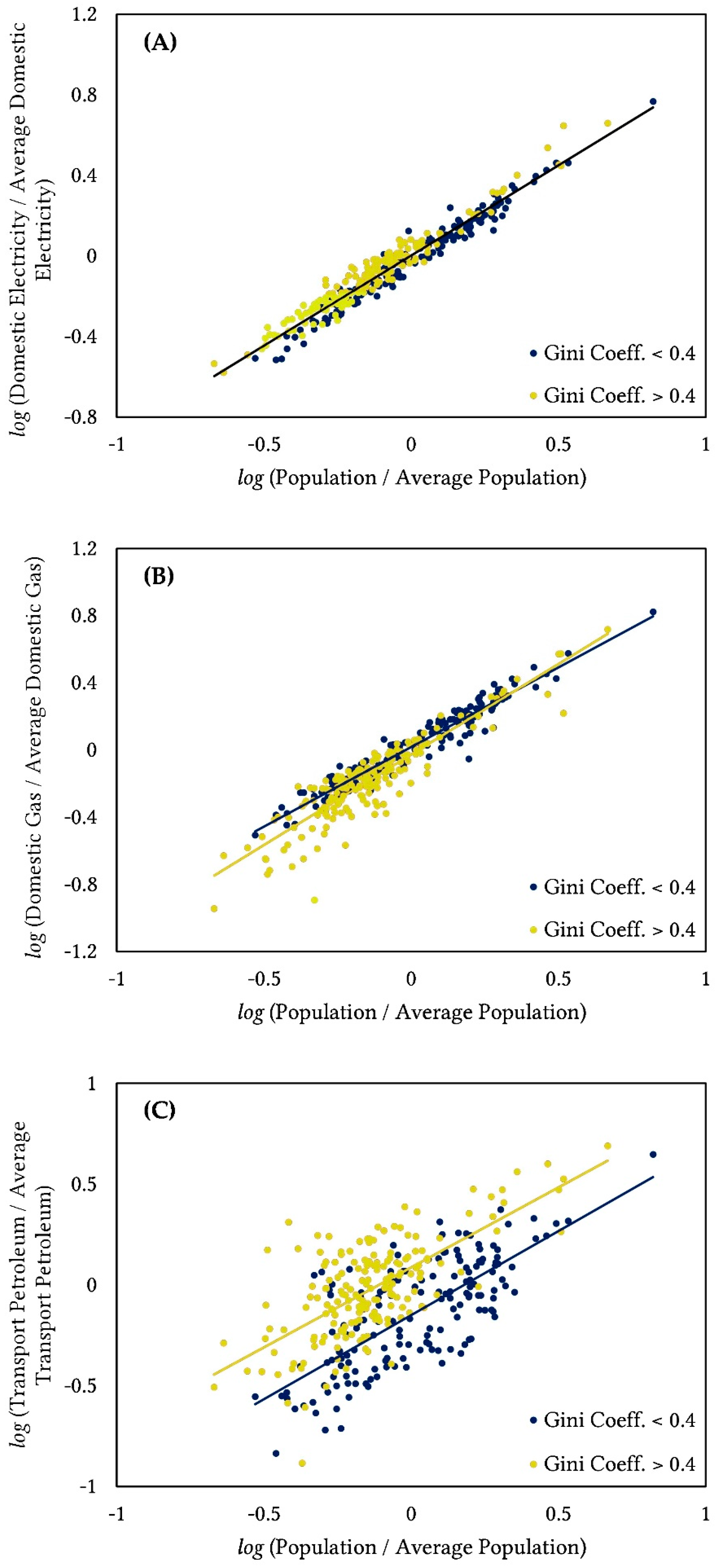
The connection between population and energy consumption across the 346 local authorities in England and Wales shows a mostly sub-linear nature. This is in agreement with the overall predictions made by Bettencourt et al. [21] that properties reflecting the production of wealth and information exhibit super-linear and those linked with built form and infrastructure in cities display sub-linear scaling with population. Although it appears fairly intuitive that there would be systematic infrastructural savings in total consumption when delivering to larger number of people on a more concentrated network (following a similar analogy to that of road networks for urban gas and electricity networks [28]), a Spanish study of electricity consumption across Andalusian settlements reports a slightly super-linear scaling [32] suggesting that unlike purely physical infrastructural characteristics, e.g., built area or length of infrastructural networks, network type, and implementation or perhaps user behavior may influence consumption behavior making its scaling context dependent and as such country specific. It should, however, be noted that the Spanish settlements considered in the study are considerably smaller than those normally considered urban, i.e., compliant with such scaling laws, with a population range of between 200 and 704,114 with the majority having less than 10,000 inhabitants.

Returning back to the findings, the tightness of the fit observed for the consumption of electricity and gas as a function of total population within the urban LAUs has an immediate implication. In their fine-resolution analysis of the UK neighborhoods, Baiocchi et al. [19] argue against the applicability of simple general models and their ability to adequately describe the dynamics behind energy consumption and CO₂ emissions in favor of a nuanced consideration of several drivers. The existence of these tight fits for the urban electricity and gas certainly signals that, at least on a macro administrative level, energy consumption dynamics are much simpler where the aggregate behavior of all inhabitants of a city relates to their total count. This is sensible when one considers that the majority of the drivers considered by Baiocchi et al. would themselves be expected to abide by various scaling relations with respect to population leaving the nuances only visible at very fine resolutions or contexts that are more driven by individual consumer behavior than the aggregated behavior of city visible in the more frequent departures from the predicted behavior of consumption in rural settings, Figure 3A.

4.1. Deviations from Expected Scaling

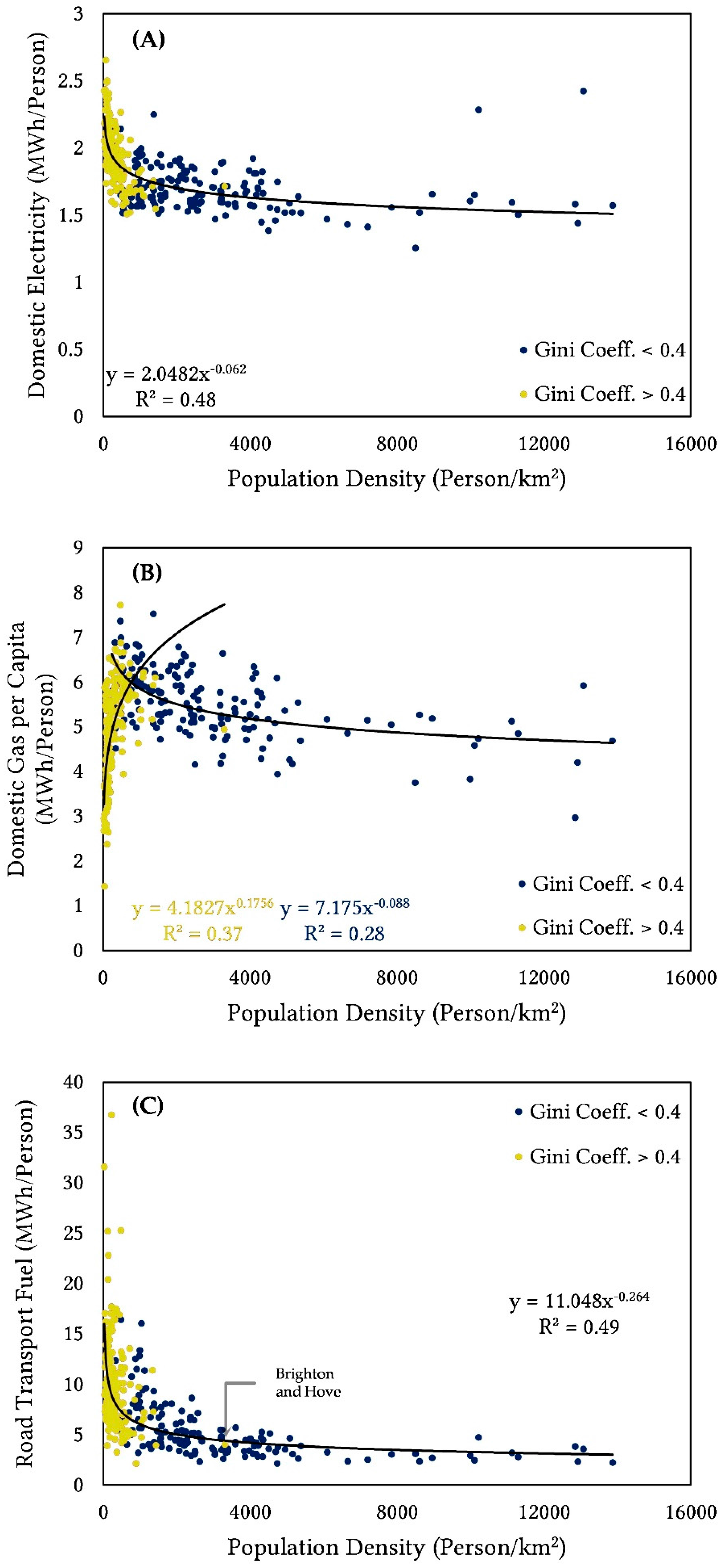
Moving on to the urban/rural differences, the super-linear exponent observed for the domestic gas consumption in rural regions can perhaps be explained by looking at the end-use of gas in the UK. The consumption of domestic gas has been indicated to largely address the space heating demand which constitutes about 70% of total domestic demand [46,47]. Heating, unlike other domestic demands, would only enjoy the effects of economies of scale when subject to more compact construction [12,15] which usually implies a smaller surface area thermodynamically and the more effective implementation of efficient heating networks. In an urban context, further increases in population can be taken as an indicator for increasing compactness of the built form and therefore higher consumption efficiencies, hence the sub-linear response of the domestic gas in the urban LAUs. In a rural setting, however, increases in total population do not necessarily translate into more compact morphologies given the nature of such settlements. In fact, the comparison of Gini coefficient and aggregate population density of the LAUs shows how the higher density urban cities also have lower Gini coefficients meaning the entirety of the population in them is focused around fewer central cores as opposed to the larger coefficients calculated for the rural authorities indicating the existence of separate and in some instances highly dispersed dense settlements. Consequently, in the absence of a decrease in surface-to-volume ratios with larger populations, larger rural entities would not exhibit a sub-linear scaling indicative of increasing efficiencies. A similar rationalization could be applied to the thermodynamically unintuitive climbing trend in the per capita consumption of domestic gas against population density for the rural areas. As already mentioned, the expectation of a decreasing trend in per capita consumption of gas, or alternatively the heating demand, is itself reliant on a sub-linear scaling of consumption with population which is in fact lacking, Equation (5).

Another issue that needs further explanation is the quality of the regression fits for the petroleum transport fuel consumption. Unlike those for the two domestic carriers, the R² of the fitted lines for transport consumption against population remains around 0.5 with relatively low slope robustness. This is also the case for the per capita consumption in the sector versus population density. Newman and Kenworthy’s [9,10] observation of the latter trend for some 32 global cities enjoys a better and tighter fit. This may partly be due to the fact that said studies only consider the fuel associated with private transport as opposed to the total road transport consumption analyzed here. However, a remaining criticism of their study and assertions has always been their consideration of population density, as a manifestation of better access, better public transportation networks, etc., as the single explaining factor driving fuel consumption [6,48]. Gordon [49] in reanalyzing their data goes on to show how economic factors such as fuel prices need to be considered as well although there does not seem to be an agreement on the extent of this dependence on economic factors as opposed to density and population related ones [50]. Returning back to the trends in the local authorities considered here, the scaling effects are undoubtedly present albeit far noisier than those seen for the total domestic demands which are unavoidable in nature and directly driven by the inhabitants and their number, the transport fuel consumption can be argued to depend on several competing factors ranging from fuel prices to vehicle ownership, road and public transport network quality, and potential traffic waiting hours. The low R² values and the scatter clouds present in the per capita consumption and density plots for the other two sectors, however, are indicative of major departures from the expected scaling relations for land area. While Bettencourt [51] puts the theoretical estimate of the areal exponent at $\frac{6}{7}$ and observed estimates [24,25,26] do mostly agree, the scaling law pertains to urbanized and/or built-up areas. The consideration of the administrative jurisdictions as functional cities in this study therefore introduces the departure from the expected scaling of area with population and, hence, the scatters seen in Figure 4.

4.2. Implications and Future Outlook

While it is important to understand the driving elements behind energy demand in cities and the possible differences in the responses of rural and urban regions highlighted in the findings here, caution must be practiced in using this understanding for policy purposes. The data provided here and the patterns and relations explored mostly suggest that there are overall savings in terms of total energy consumption associated with higher density urban settings. This on face value could lead to simple advocacy for a preference in higher density developments. It, however, should be noted that at least for the network of cities in England and Wales despite the clear existence of these trends the practical savings may not be worth other potential technical and socioeconomic expenses [52] as each 1% increase in population density only results in approximately 0.3% and 0.06% decreases in per capita transport and domestic electricity consumption, respectively. This is in contrast with the theoretical savings of up to 1.12% and 0.4% respectively, from the exponent in Equation (5), were the built-up area of the urban LAUs considered rather than their administrative boundaries. What could be used in terms of a practical lesson from the urban/rural differences seen here is the potential in better understanding the properties of the infrastructural networks implemented in denser urban cities and borrowing from them, particularly in the transport sector where the overall consumption dynamic appears to be similar despite the higher baseline consumption of the rural regions, Figure 3, for the future infrastructural developments and investments within the rural authorities in an attempt to reduce the total consumption share of these regions.

Lastly, the existence of these scaling effects also brings up further questions. Bettencourt et al. [21] and Bristow and Kennedy [53] explore possible future growth scenarios in terms of the carrying capacity of resources, e.g., social interaction, energy, GDP, etc., and population growth and also the effects of similar scaling laws between the economy of cities and their energy consumption. The study presented here explores the trends and the divide between the urban/rural consumption behavior and population for a single snapshot of England and Wales in 2011. Future works will explore the existence of potentially similar trends in a time series dataset, where the evolution of consumption patterns across the urban and rural regions can be observed both within particular settlements and across the entirety of England and Wales as a whole, and ask three questions: (i) Is there a limiting capacity to the growth of settlements where energy consumption is concerned especially in the rural areas? (ii) Is there an economic limit, based on similar power laws, to the growth of cities based on their consumption patterns? (iii) Do urban and rural authorities keep to similar general scaling patterns going back in time?