1. Introduction
The role of Heating Ventilation and Air-Conditioning (HVAC) systems and controls within a building is an important one as it has significant impact on the energy consumption and internal comfort [
1]. HVAC systems with efficient control increases the productivity and comfort satisfaction of a building’s occupants [
2]. In terms of cost and energy savings, a reduction of up to 30% can be achieved [
3]. Thus, it is of utmost importance for designers to make informed decisions on the choice and design of HVAC systems and controls [
4] to take into consideration both energy and comfort requirements.
Advances in computing technology have led to the possibility of modelling sophisticated controls and system performance in great detail. However, building energy simulation tools today are rigid and lack flexibility in terms of modelling a variety of HVAC systems and control options. As a result, this limits practitioners from exploring various system design and control strategies and deters them from seeking alternative system designs that could reveal opportunities to save energy.
This research builds on previous research by investigating the performance of a complete (primary and secondary) heating system developed specifically for a third-order lumped parameter building model [
5]. Primary plant refers to the source of heat energy, such as conventional boilers, biomass boilers, and heat pumps, The model allows three possible configurations of primary plant, namely conventional only (boilers), renewables only, or hybrid (boilers and renewables). Secondary plant refers to room-based equipment that is used to distribute the heat energy to the occupants, such as underfloor heating and radiators. The model is capable of adopting all of the common control strategies for these secondary plant items and is applicable to any commercial or residential building which has a heating system.
2. Modelling of HVAC Systems and Controls
HVAC systems and controls are traditionally modelled using either menu-based or component-based tools to cater for different levels of user skills and modelling capabilities. Of the two, the menu-based approach is a simple and straightforward method adopted by most tools such as DOE-2, eQuest, Building Analyser, BLAST, and DesignBuilder which is a graphical user interface for the extensively-used EnergyPlus simulation engine. This approach provides preconfigured and packaged heating/cooling systems that are represented in the form of a menu for users to insert the parameters.
The component-based system approach requires users to have a deeper understanding of HVAC systems as it provides greater flexibility in terms of system customization. Good examples of tools adopting this approach are IES-APACHE and TRNSYS. Each system is represented by individual components encapsulated with mathematical algorithms and energy balancing equations where the output of each component is connected to the input of the next component to make up a system [
6].
For the purpose of comparing HVAC systems and evaluating different control strategies, detailed dynamic HVAC models are required [
7,
8,
9,
10,
11]. These detailed dynamic HVAC models have higher explicitness, thus requiring a greater number of user input parameters and in-depth specialist knowledge of controls. In addition, many tools available today use a fictitious and immeasurable parameter as an input parameter for the controller such as the use of the exact energy demand (so-called “heat-balance models”) to achieve the setpoint.
Previous research [
12] successfully developed a user-friendly, dynamic heat emitter model that has achieved improved results when compared to commercially available tools, such as IES and EnergyPlus. This research expands on previous work to inform sustainability engineers and modelers of the energy performance of alternative heating systems and showcases a range of control strategies available.
The objectives for this research are as follows:
- (1)
Develop robust circuit control strategies with multi-zone functionality commonly adopted in current design practice for secondary system side and advanced system control strategies;
- (2)
Embed primary and secondary HVAC systems and component models within parent code; and
- (3)
Test and demonstrate the capabilities of the primary and secondary HVAC systems adopting a wide range of control strategies and primary plant system configurations.
3. Development of HVAC Systems and Controls
The following commonly-used control strategies have been developed for the purpose of this research. These control strategies are easy to implement allowing modelers to make comparative assessment in terms of comfort and energy:
- (1)
Constant Temperature, Varying Flow rate (1CTVF), typically used in zone feedback control;
- (2)
Varying Temperature, Constant Flow rate (2VTCF), typically used in weather-compensated control;
- (3)
Varying Temperature, Varying Flow rate (3VTVF), typically used when both of the above methods are combined; and
- (4)
Constant Temperature, Constant Flow rate (4CTCF), typically used in simple thermostatic (i.e., “on-off”) control.
3.1. Variable Flow Rate
The variable flow (VF) rate control is most commonly found on domestic radiators where a thermostatic radiator valve (TRV) regulates the flow rate into the emitter by adjusting the valve. (The term “thermostatic” in this context is a misnomer because these types of valves vary the flow rate to each radiator in response to local room temperature conditions). This method of control takes the internal temperature of the treated zone as an input to control the flow rate. Flow rate is regulated linearly between zero and the designed mass flow rate with reference to the deviation between the upper and lower limits of the proportional band imposed on the setpoint, also known as the throttling range. Once the internal temperature reaches above the upper limit, when heating is no longer required, the controller delivers zero flow, turning the emitter off. Conversely, the heat emitter receives the designed mass flow rate to provide maximum thermal output when the internal temperature is below the lower limit. Equation (1) shows the calculation method to determine the mass flow rate when varying:
3.2. Variable Temperature
Variable (VT) temperature control, better known as weather-compensating control, modulates flow temperature in accordance to the external temperature [
13]. This method of control is frequently adopted in the UK [
14] because it has a low installation cost and enables the heating system to be adjusted in relation to the coldness of the weather [
15].
The external dry bulb temperature and the flow temperature are required as inputs for the weather compensating control to function. The flow temperature serves as a feedback input to ensure the required temperature is met. The flow temperature, which varies between the design water temperature and minimum flow water temperature, is linearly proportional to the design external dry bulb temperature (typically, −3 °C) and a balance point temperature [
12], shown in Equation (2). The balance point temperature refers to an external temperature, typically 15–20 °C dry bulb temperature, where heating is no longer required [
15]. The minimum flow water temperature is dependent on the type of emitter. Typical minimum flow water temperatures for radiators and underfloor heating are 20 °C and 35 °C respectively [
15,
16].
3.3. Constant Temperature and/or Constant Flow Rate
The control strategies 1, 2, and 3 developed for the emitter models have either flow temperature and/or the flow rate varying. Emitters adopting strategies with constant flow (CF) temperature will receive water temperature at design value dependent on the type of emitter, typically 80 °C for radiators and 45 °C for underfloor heating.
Similarly, constant flow rate control circuits will be supplied with the designed mass flow rate. Control strategy 4, with constant temperature and constant flow (CTCF) control, better known as ON/OFF thermostatic control, toggles between fully on when the internal zone temperature falls below the heating setpoint, and fully off when it is above the setpoint.
3.4. Assumptions for Primary HVAC Systems
The following assumptions are made for the primary HVAC systems and controls developed for this research and for the other software used for comparison:
All emitter systems are connected to a single main circuit on the secondary side;
A maximum of three units of primary plant have been specified for each of the heating systems tested and compared in this research;
Pressure loss effects in pipe fittings and plant are neglected;
The schedule controller is designed to offer the minimum number of primary plant (e.g., boilers) to satisfy load requirements;
Loads are shared equally between the online primary plant;
Flow rate entering the primary plant is constant; and
Required flow water temperature by the secondary systems is constantly met.
3.5. Modelling of Primary HVAC Systems
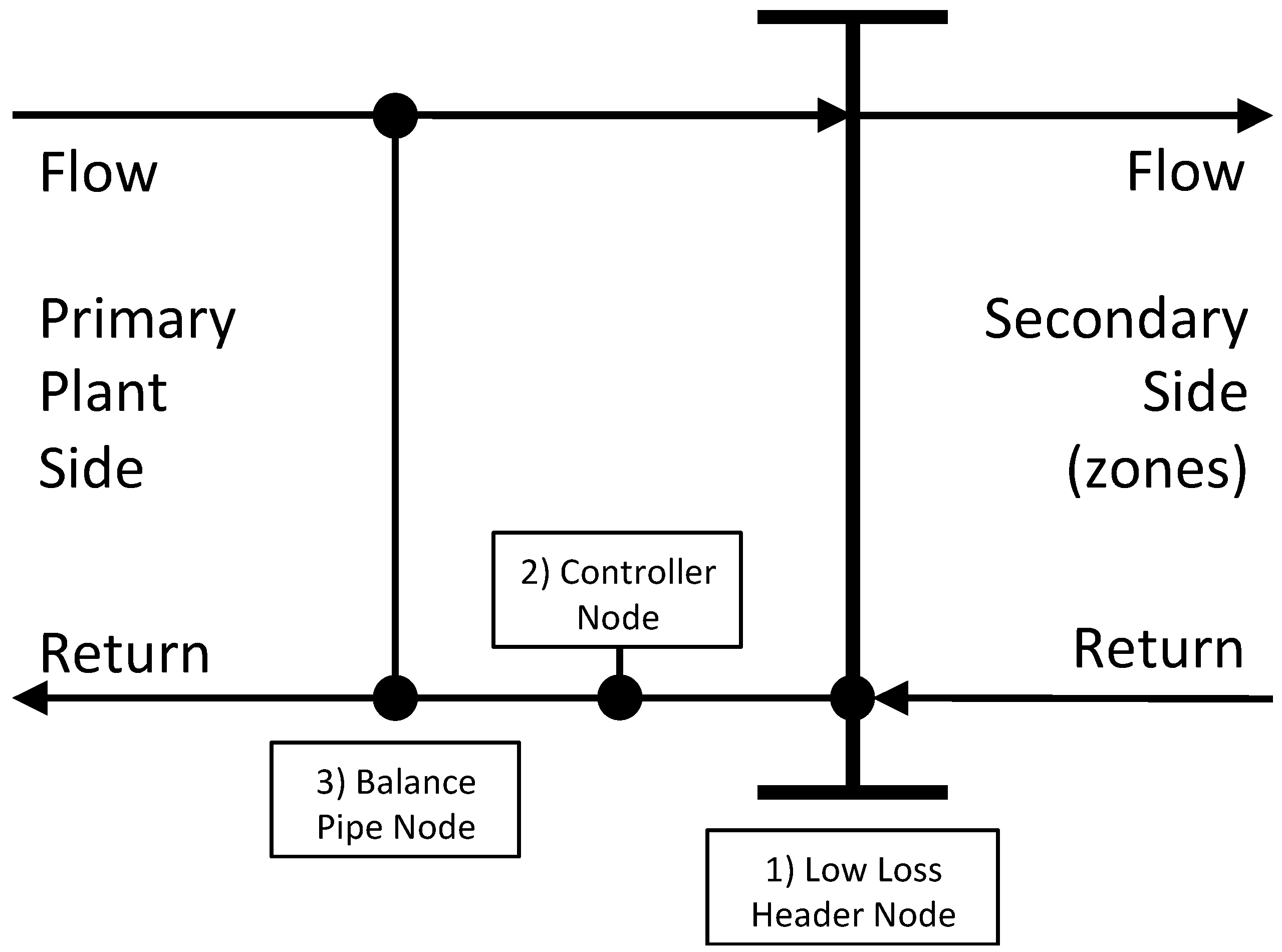
Modelling of the primary plant for this research is carried out in three stages by passing parameters from one node to the next as illustrated in
Figure 1 below. Node, in this context, refers to a conjunction point where variables are passed from one model/side to another stage. The first stage at the (1) Low Loss Header Node is where variables from the secondary system side are passed to the primary side (heat generator (s)). These parameters are fed into the next stage at the (2) Controller Node to determine the status (es) of the generators/s based on energy demand from the building. Lastly, the flow rates between the flow and return sections on the primary side are balanced in the (3) Balance Pipe Node.
3.5.1. Step 1: Low Loss Header Node
The low loss header node is an intersection point that balances the flow rates and temperatures between primary plant and secondary systems. Variables for the primary side are calculated using return outputs from the secondary side at the low loss header node. For future expansion, secondary systems, such as domestic hot water (DHW) and heating coils for all air systems, can be easily connected to the low loss header node.
(a) Weighted average return water temperature across all zones
The weighted average of the return water temperature is a single return water temperature from all secondary circuits returning to the primary system calculated using Equation (3):
(b) Sum of total mass flow rate of all zones
Mass flow rates for all treated zones are summed as an input for the boiler model using Equation (4):
3.5.2. Step 2: Controller Node
The modulating sequence controller determines the operational status and percentage load capacity of the primary plant side using the input parameters calculated at the low loss header. The energy demand of the secondary systems is shared equally amongst the online primary plant to meet the load demand.
At the start, all three generators are offline when loads are below the assumed 25% (i.e., the assumed minimum turn-down ratio) of the lead generator. Once the load increases to above 25% of the maximum generator capacity, the lead generator comes online. When the load exceeds the lead generator’s maximum capacity, the sequence controller will schedule the next generator to come online and share the total load equally. The same process is repeated when the load exceeds the capacity of two generators and the third generator will be brought online to share the load equally.
Primary Plant Systems Configurations
The various configurations of primary plant are one of the highlights of this paper. It allows users to model different plant combinations to conduct comparative analysis on their energy performances. Three possible primary plant configurations as shown below have been developed for this research. Users would simply select one configuration from the three options available. For the hybrid system plant configuration, the low carbon renewable system(s) will serve as the lead with the conventional plant topping-up.
- (1)
Conventional system(s) only;
- (2)
Renewables system(s) only; and
- (3)
Hybrid system(s).
3.5.3. Step 3: Balance Pipe Node
The balance pipe is used to balance the flow rates between the flow and return streams of the primary side. Depending on the number of generators online, the flow rate required by the return stream entering the plant can be determined and the excess flow rate between the flow and return streams is automatically balanced by the balance pipe.
When the flow rate required by the plant is less than the flow rate on the return side, the excess flow rate is diverted away from the return to the flow stream in the balance pipe. This would result in cooler return water mixing directly to the flow stream and is compensated by the plant generating higher supply temperature.
Conversely, when the plant requires additional flow rate to operate, flow is directed from the supply stream with the higher temperature and mixed directly with the cooler return stream, raising the temperature of the flow entering the plant.
3.6. Development of Primary Plant Models
Three primary plant models have been developed for this research:
3.6.1. Development of Conventional and Biomass Boiler Models
The boiler model developed for this research adopts the British European Standards (BS EN 15316 series) for development of conventional boilers [
17] and biomass boilers [
18]. The standard is in compliance with the Council Directive 92/42/ECC regarding boiler efficiency [
19].
The model has a convenient setup which requires a total of only four input parameters by the user. These are the type of boiler (conventional low temperature or condensing), burner (atmospheric, fan-assisted, gas or oil), location (room temperature or naturally ventilated space) and, lastly, boiler capacity.
In each of the BS EN standards, three steady state methods with increasing complexities have been detailed. The intermediate complexity boiler efficiency calculation method has been adopted for this research as it offers more detail than the simpler method whilst not requiring iteration/loops that will add to the computational effort found in the more complex method.
The method consists of a total of 21 and 29 calculations steps for the conventional boiler and biomass boiler as detailed in Appendix F of British European Standard 15316: 4:1 and Appendix A of British European Standard 15315: 4:7 respectively. The calculation steps for both conventional and biomass boiler types can be categorized into three main sections. The first section consists of calculation steps to generate parameters that are kept constant throughout the simulation at full, intermediate, and zero load points, such as boiler efficiency and thermal losses. The second section adjusts the efficiencies, thermal losses, auxiliary power, and fuel consumption with reference to the load using interpolation at each time-step. Finally, the latter variables are summed and scaled up by multiplying by the number of operational hours to calculate overall energy performance.
This procedure is re-calculated and updated at each time-step providing a realistic representation of the system over a full operating cycle of the plant after which the results are integrated to form operating cycle total energy consumptions, etc.
3.6.2. Development of Heat Pump Models
The heat pump models developed for this research have been curve-fitted from manufacturer’s data [
20]. At each time-step, the equation below is used to determine the load on the evaporator/condenser and compressor by assuming a 5K temperature difference.
A,
B,
C,
D,
E,
F are coefficients obtained from the regression curve fitting method and models fitted for the purpose of this research and can be found in
Table 1. These heat pump models have been selected based solely on the capacity of the systems and availability of the data. Subsequently, the coefficient of performance (CoP) can be determined. For further details of this method, see [
21]:
where:
: external dry bulb temperature (°C);
: return water temperature (°C).
4. Testing/Debugging of Primary Plant Models
Tests were carried out independently on separate components using manual calculations and analytically verified on a spreadsheet. The systems are then integrated as a complete heating primary-side system and extensively tested by manually stepping through the code for various possible scenarios to ensure the robustness and functionality of the model.
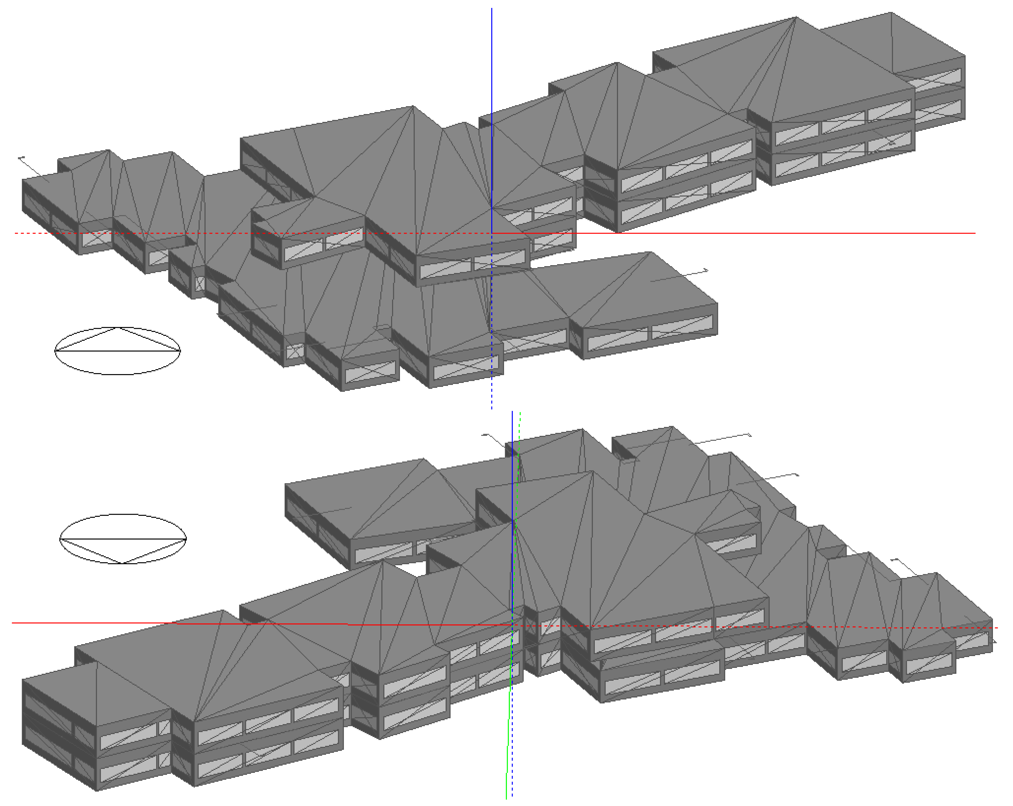
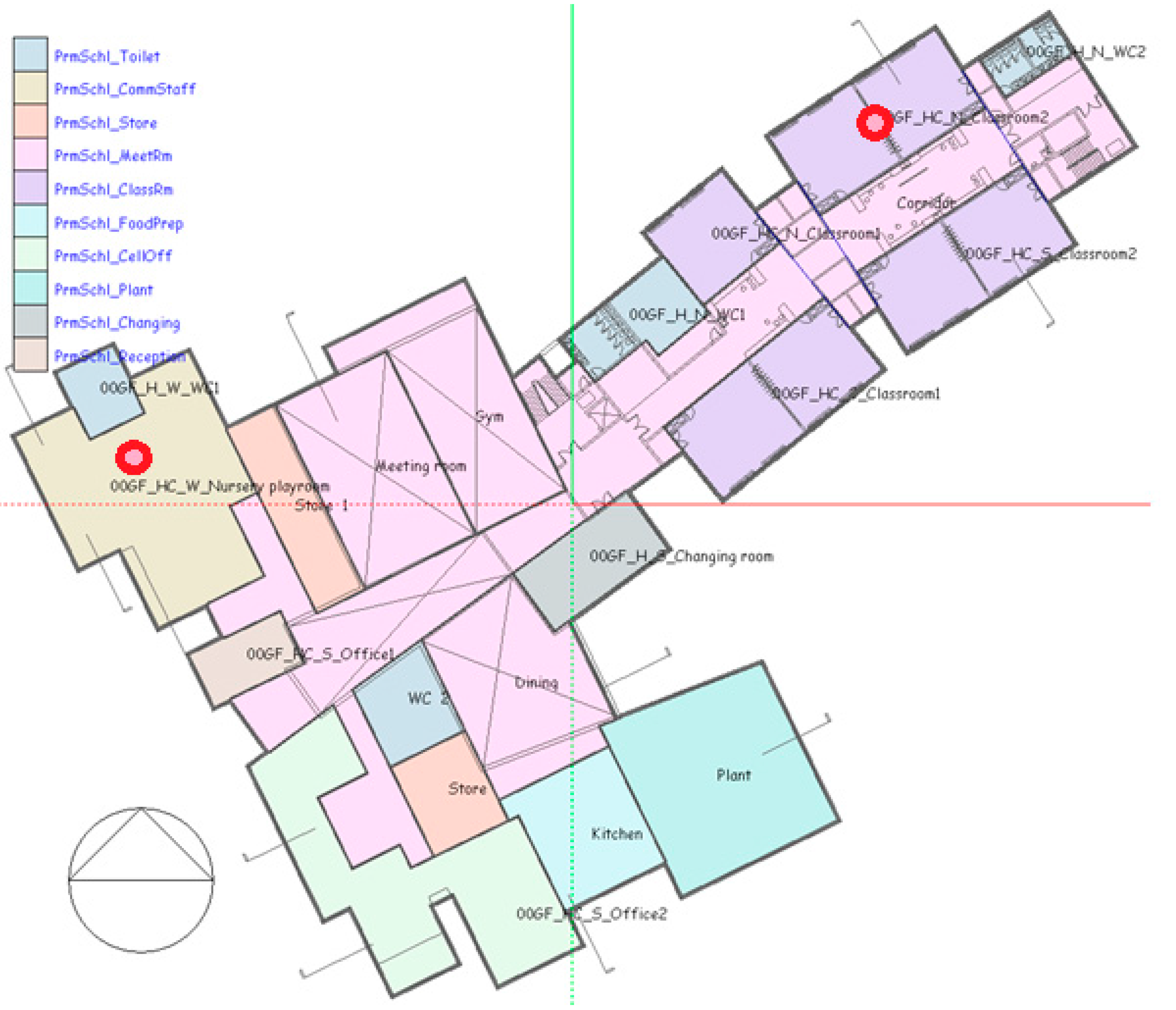
4.1. Test Case Building Model
For the purpose of this research, a naturally-ventilated 25-zone actual school building, shown in
Figure 2 and
Figure 3, with a gross floor area of 4870 m
2 has been adopted [
22]. The models developed for this research are tested against EnergyPlus (version 7.2.0.006, U.S. Department of Energy, Washington D.C., U.S.) and IES VE (version 6.4.0.10, Integrated Environmental Solutions, Glasgow, U.K.), two building energy modelling tools widely used in both academia and industry. Inter-model comparison [
23] is an accepted tool to verify simulation software results.
The building was first modelled in DesignBuilder (version 3.1.0.089, DesignBuilder Software Ltd., Stroud, U.K.) and exported to XML format, which was further modified to incorporate the detailed HVAC module developed for this research. In order to fully embed the developments of this research, modifications had to be made to the XML schema, which contains the input parameters of the systems and the source code of the third order lumped parameter building model to read the input parameters. The HVAC module developed for this research is fully embedded within the simulation tool that reads and calls upon the relevant modules when required.
For simulations in EnergyPlus, the same model developed in DesignBuilder was used and exported to IDF format. For further comparison the same information was used to create an identical model in IES VE.
Results from two key zones (Nursery and Classroom) on the ground floor have been selected as indicated (red dots) in the floor plan above to provide results for zones with different usage patterns. Simulations were performed using a local Newcastle weather file [
24,
25] for the building which adopts construction templates used in the COPSE Project [
22] shown in
Table 2.
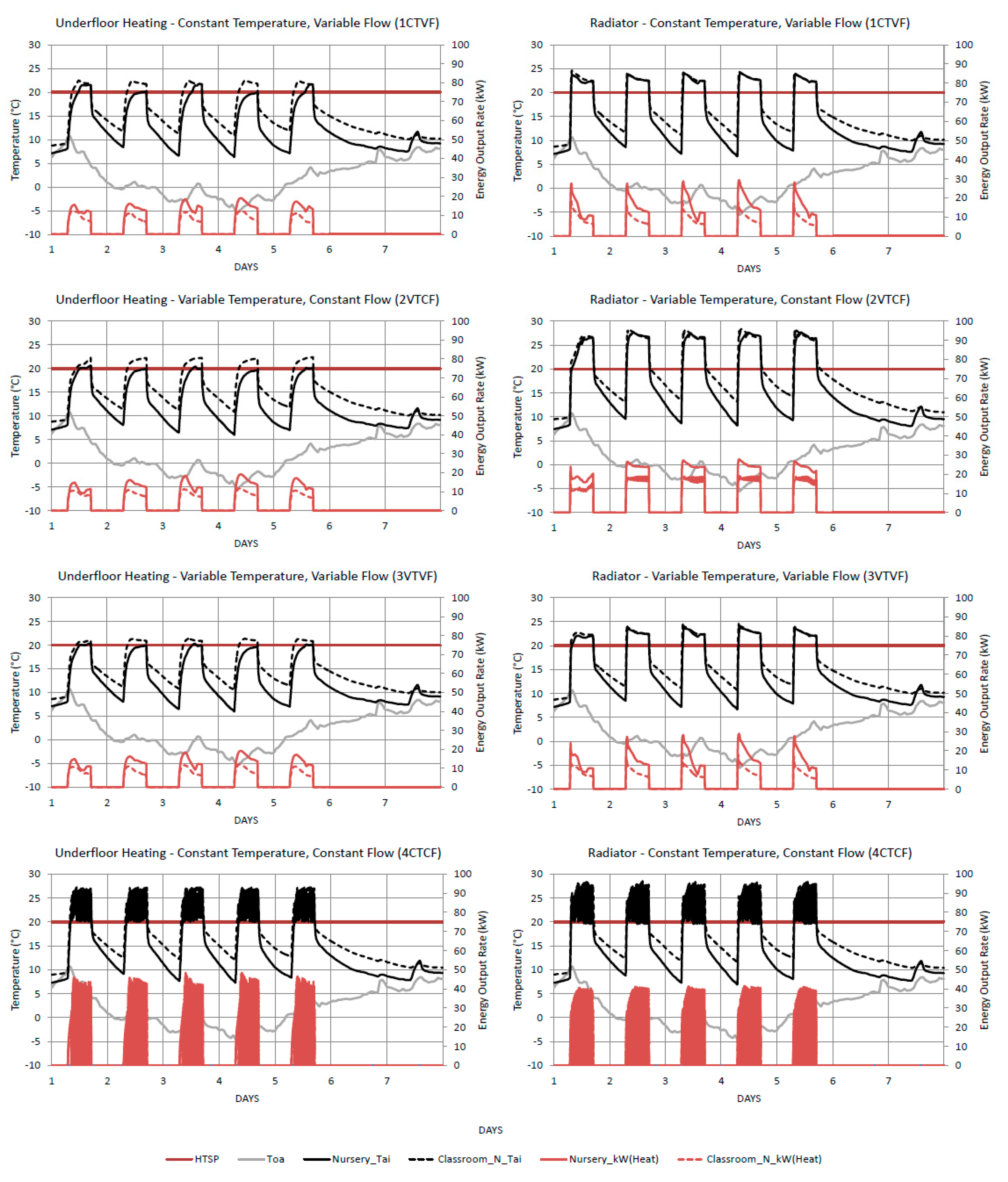
Temperature profiles and energy output rates for the variants in the table listed below (
Table 3) have been presented. Parameters investigated are emitters with different thermal capacities, various control strategies and primary plant configurations. Results are presented for a peak winter week with a typical day extracted providing a clearer representation of the emitter and control strategies in terms of temperature and energy profiles.
4.2. Thermal Comfort
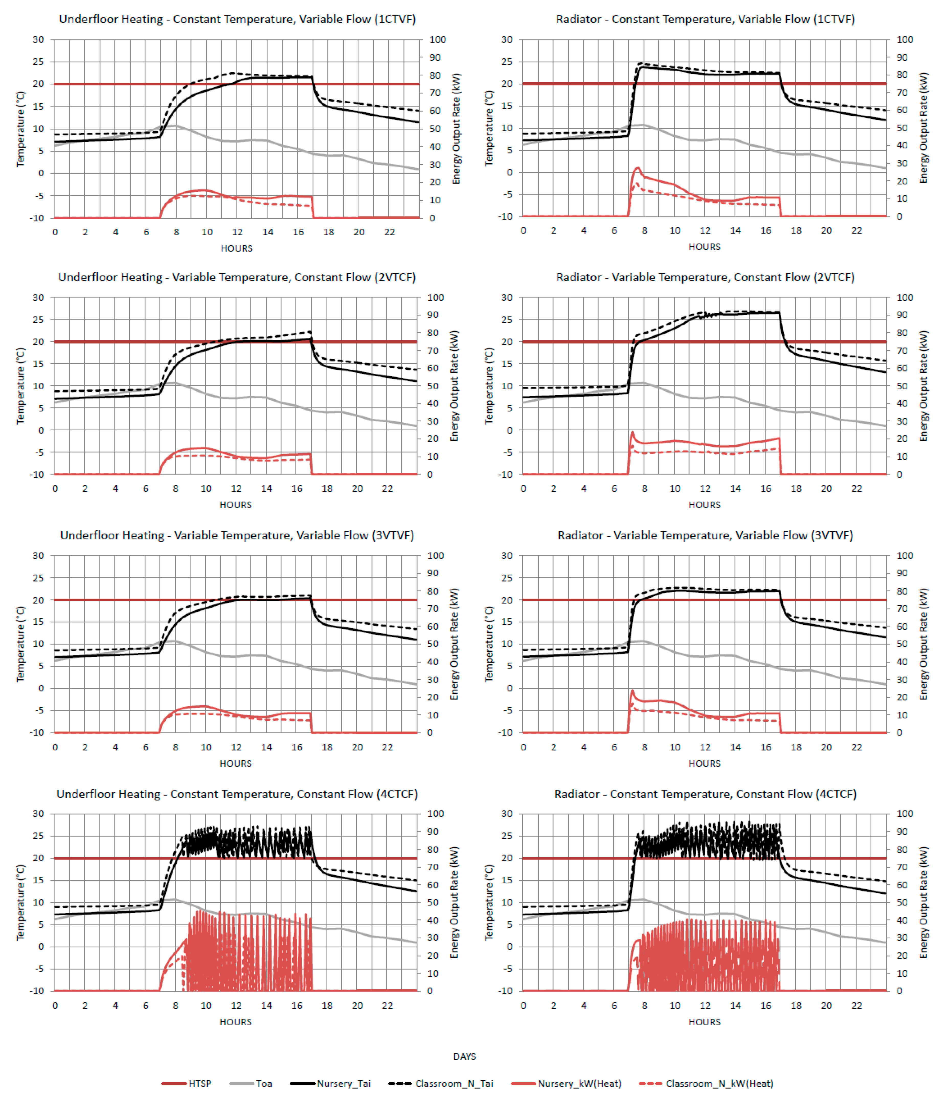
Figure 4 and
Figure 5 present results generated for underfloor heating (left column) and radiators (right column) for various control strategies (top to bottom) for a peak winter week. Looking from top to bottom at the various control strategies imposed on the emitters, it is clear that the first three control strategies are capable of successfully achieving the setpoint temperature of 20 °C and demonstrate stable results throughout the peak winter week. Circuit 4 however is the thermostatic control and the inherent deviations in controlled temperature (often known as “saw-toothing”) are clearly evident.
Comparing underfloor heating and radiators (left and right), the ability of the model to capture the transient effects and thermal responsiveness of both emitters can be seen. The radiator model can be seen to achieve the setpoint at a quicker rate of within 30 min (
Figure 5) compared to the underfloor heating system which can take up to two hours or more to achieve the heating setpoint of 20 °C.
The higher responsiveness of the radiator is accurately captured in the weather-compensating Variable Temperature, Constant Flow (2VTCF) control strategy. This method of control often causes overheating because it is based on an external dry bulb temperature without accounting for the zone’s internal temperature and useful internal heat gains.
4.3. Energy Consumption by Primary Plant
This research developed a convenient, and yet rigorous, approach to model different control strategies and switch between conventional, renewables, and hybrid plant configurations to evaluate energy consumption. Heating energy consumption calculated over the treated floor area is presented in
Table 4 for various emitters, circuit controls, and plant configurations.
Energy benchmarks for a primary school building are 164 kWh/m
2 fuel and 32 kWh/m
2 electricity for typical practice, and 113 kWh/m
2 fuel and 22 kWh/m
2 electricity for good practice [
26] over the treated area. Results in
Table 4 show that the energy predictions made by the detailed HVAC module developed for this research are within limits of good and typical practices for the test scenarios, as recommended by CIBSE [
26].
On closer examination, it is evident that the constant temperature and constant flow rate thermostatic control requires significantly more energy when compared to other strategies. This is due to the nature of the controller as it toggles between maximum capacity instead of modulating between proportional bands (VF) and/or in accordance to the external temperature (VT). The high frequency of delivering heating at maximum capacity has thus led to higher energy consumption.
Energy consumption by the radiator system is larger when compared to the underfloor heating system when adopting weather-compensated control. Other than operating at different flow and return water temperatures between the systems, the higher energy consumption by the radiators is largely caused by the higher thermal responsiveness of the emitter causing conflicts between heating and cooling systems.
Unlike weather-compensated control (2VTCF), 1CTVF and 3VTVF take into account zone internal temperatures. In the case of constant temperature variable flow (1CTVF), the underfloor heating system is seen to consume more energy than the radiator system. This is mainly due to the systems having a different response time influenced by the emitter’s thermal capacity. The difference in heating energy profile is governed by the response time of the emitter (
i.e., thermal capacity) in which a lesser amount of energy is required by the fast responding radiator and a larger amount of energy is required to overcome the thermally-heavy underfloor heating system. In addition to the mathematical representation for each of the control strategies in previous work by Fong
et al. [
12], the table below (
Table 5) summarizes the advantages and disadvantages for each of the strategies based on energy consumption.
5. Conclusions
The aim of this research was to demonstrate a new building energy modelling method capable of conveniently dealing with alternative control strategies and generating plant options. The results presented here are based on the modelling procedure described in [
12] to enable the study of energy consumption in heating systems. A case study was modelled in order to demonstrate the full capabilities and functionalities of the new method. Temperature profiles and energy consumption for different emitters adopting various circuit control strategies are presented.
A number of zone and system control configurations have been simulated over a range of possible primary plant configurations. It has been shown that these are convenient to implement and that this enables comparative evaluation of various plant configurations (including hybrid schemes) to be conducted. Predictions of temperatures made by the various control circuits have demonstrated the ability to provide a realistic representation of how the controllers work in the real world and the results generated compare favorably with established benchmark data.
6. Limitations
The authors recognize that this research is limited by the functionality of each given modelling tool in terms of detail and calculation methods. Furthermore, the validity of the results from this research is based upon inter-model comparison [
23] with tools widely used in industry which could be verified further with empirical measurements.
7. Future Work
The recommendations for future research are as follows:
Extend the control options at primary system level to include advance control options;
Extend the library of components to encompass a larger variety of primary system types;
Conduct empirical validation of the new program; and
Modify the detailed HVAC module to incorporate sophisticated features in C++ for better memory management to further improve computational efficiency.
Acknowledgments
The authors would like to thank DesignBuilder Software Ltd. for their technical support and financial assistance for this work.
Author Contributions
Joshua Fong did the modelling and had an equal contribution to paper authorship with Jeremy Edge. Chris Underwood provided advice and editorial support. Andy Tindale and Steve Potter supplied the parent code used in the analysis and also advised on modelling. Hu Du provided formatted weather data for use in the simulations.
List of Symbols
| zone index |
| emitter mass flow rate (kg/s) |
| emitter mass flow rate at design (kg/s) |
| emitter return mass flow rate (kg/s) |
| sum of mass flow rate (kg/s) |
| proportional band (Kelvin) |
| external dry bulb temperature at current time-step (°C) |
| external dry bulb temperature at design (°C) |
| internal air temperature (°C) |
| balance point temperature (°C) |
| emitter flow water temperature at current time-step (°C) |
| emitter flow water temperature at design (°C) |
| emitter flow water temperature at minimum (°C) |
| emitter return water temperature (°C) |
| emitter weighted return water temperature (°C) |
| Z | total number of zones |
References
- Haines, R.W.; Hittle, D.C. Control Systems for Heating, Ventilating, and Air Conditioning, 5th ed.; Van Nostrand Reinhold: New York, NY, USA, 1993. [Google Scholar]
- Andre, P.; Hannay, C.; Hannay, J.; Lebrun, J.; Lemort, V.; Teodorese, I.V. A contribution to the audit of an air-conditioning system: Modelling, simulation and benchmarking. Build. Serv. Eng. Res. Trans. 2008, 29, 85–98. [Google Scholar] [CrossRef]
- Tashtoush, B.; Molhim, M.; Al-Rousan, M. Dynamic model of an HVAC system for control analysis. Energy 2005, 30, 1729–1745. [Google Scholar] [CrossRef]
- Platt, G.; Li, J.; Li, R.; Poulton, G.; James, G.; Wall, J. Adaptive HVAC zone modelling for sustainable buildings. Energy Build. 2010, 43, 412–421. [Google Scholar] [CrossRef]
- Tindale, A. Third order lumped-parameter simulation method. Build. Serv. Eng. Res. Technol. 1993, 14, 87–97. [Google Scholar] [CrossRef]
- Tahersima, F.; Stoustrup, J.; Rasmussen, H.; Nielsen, P.G. Thermal analysis of an HVAC system with trv controlled hydronic radiator. In Proceedings of the IEEE Conference on Automation Science and Engineering (CASE), Toronto, ON, USA, 21–24 August 2010.
- IEA. Task 12: Empirical Validation of Thermal Building Simulation Programs Using Test Room Data; IEA21RN399/94; IEA: Cedar, MI, USA, 1994. [Google Scholar]
- Hensen, J.L.M. Application of modelling and simulation to HVAC systems. In Proceedings of the 30th International Conference MOSIS’96, Mumbai, India, 3–6 September 1996.
- Hanby, V.I. Simulation of HVAC components and system. Build. Serv. Eng. Res. Technol. 1987, 8, 5–8. [Google Scholar] [CrossRef]
- Nassif, N.; Moujaes, S.; Zaheeruddin, M. Self-tuning dynamic models of HVAC system components. Energy Build. 2008, 40, 1709–1720. [Google Scholar] [CrossRef]
- Trcka, M.; Hensen, J.L.M. Overview of HVAC system simulation. Autom. Construct. 2010, 19, 93–99. [Google Scholar] [CrossRef]
- Fong, J.; Edge, J.; Underwood, C.; Tindale, A.; Potter, S. Performance of a dynamic distributed element heat emitter model embedded into a third order lumped parameter building model. Appl. Ther. Eng. 2015, 80, 279–287. [Google Scholar] [CrossRef]
- Day, A.R.; Ratcliffe, M.S.; Shepherd, K.J. Heating Systems: Plant and Control; Blackwell Publishing: Oxford, UK, 2003. [Google Scholar]
- Harvey, J. Satchwell: Controls for Building Services: An Introductory Guide, 2nd ed.; Satchwell Control Systems: Berkshire, UK, 1993. [Google Scholar]
- Levermore, G.J. Building Energy Management Systems: An Application to Heating and Control; E&FN Spon: London, UK, 1992. [Google Scholar]
- CIBSE. Application Manual 14: Non-Domestic Hot Water Heating System; The Charlesworth Group: West Yorkshire, UK, 2010. [Google Scholar]
- Bs en 15315-4-1: Heating Systems in Buildings—Method for Calculation of System Energy Requirements and System Efficiencies. Part 4-1: Space Heating Generation Systems Combustion Systems (Boilers); BSI Group Headquarters: London, UK, 2008.
- Bs en 15315-4-7: Heating Systems in Buildings—Method for Calculation of System Energy Requirements and System Efficiencies. Part 4-7: Space Heating Generation Systems Biomass Combustion Systems; BSI Group Headquarters: London, UK, 2008.
- Council Directive. 92/42/ecc: On Efficiency Requirements for New Hot-Water Boilers Fired with Liquid or Gaseous Fuels; The Council of the European Comunities: Brussels, Belgium, 1992. [Google Scholar]
- CIAT. Universal Comfort na 07.01a. Available online: http://www.ciatozonair.co.uk/rubrique/index/eng-catalogue/33/AQUACIAT2-HYBRID/2191 (accessed on 31 May 2015).
- Underwood, C.P.; Yik, F.W.H. Modelling Methods for Energy in Buildings; Blackwell: Oxford, UK, 2004; pp. 135–152. [Google Scholar]
- Levermore, G.J.; Watkins, R.; Cheung, H.; Parkinson, J.; Laycock, P.; Natarajan, S.; Nikolopoulou, M.-H.; Mcgilligan, C.; Muneer, T.; Tham, Y.W.; et al. Deriving and Using Future Weather Data for Building Design from UK Climate Change Projections: An Overview of the COPSE Project; University of Manchester: Manchester, UK, 2012. [Google Scholar]
- Bowman, N.T.; Lomas, K.J. Empirical validation of dynamic thermal computer models of buildings. Build. Serv. Eng. Res. Technol. 1985, 6, 153–162. [Google Scholar] [CrossRef]
- Du, H.; Underwood, C.P.; Edge, J.S. Generating test reference years from the UKCP09 projections and their application in building energy simulation. Build. Serv. Eng. Res. Technol. 2012, 33, 387–406. [Google Scholar] [CrossRef]
- Du, H.; Underwood, C.P.; Edge, J.S. Generating design reference years from the UKCP09 projections and their application to future air-conditioning loads. Build. Serv. Eng. Res. Technol. 2012, 33, 63–79. [Google Scholar] [CrossRef]
- CIBSE. Guide F: Energy Efficiency in Buildings, 3rd ed.; Page Bros Ltd.: Norwich, UK, 2012. [Google Scholar]
© 2016 by the authors; licensee MDPI, Basel, Switzerland. This article is an open access article distributed under the terms and conditions of the Creative Commons Attribution (CC-BY) license (http://creativecommons.org/licenses/by/4.0/).


