1. Introduction
The EU 2030 emissions reduction target of 40% [
1] requires significant changes in the residential sector, which accounts for 1/3 of energy usage [
2]. A move from the dominant gas heating common in many EU member states, such as the UK [
3], to lower carbon heating from a range of heating equipment will necessitate a more complex decision making process by consumers and specifiers during selection of heating systems. The European Commission provides the Energy Performance of Buildings Directive (EPBD) as a framework for simplified static models to assess retrofit activities and provide the decision maker with information about predicted energy consumption [
4]. EU member states are required to implement building Energy Performance Certificates (EPC) utilising results from the use of National Calculation Methods (NCM).
Discrepancies between calculated energy consumption and that experienced during building use are well documented in the literature [
5]. Residential, non-domestic [
6,
7] and historic buildings [
8] all show a gap between the predicted and actual energy consumption. The energy consumption calculated by NCMs follows the same trend has been observed [
9,
10].
This performance gap has been widely investigated, including behavioural aspects (comfort taking, rebound) [
11] and technological aspects outside the core technology (installation issues, building regulations, control mechanisms) can all lead to lower or higher than expected energy use, often described under the umbrella of “rebound” [
11]. However, reliable estimation of the energy savings, through the appropriate use of models, is central to minimizing this performance gap [
5].
SAP (Standard Assessment Procedure) is the designated NCM for UK domestic properties, SAP Version 2009 [
12] is based around a monthly heat balance model using average internal and external temperatures. SAP is derived from the established BREDEM model (Building Research Establishment Domestic Energy Model), which has been well documented [
13]. SAP has been compared to a dynamic model (Inverse Dynamics Energy Assessment and Simulation, IDEAS) by Murphy [
14] showing similar predictions of the relative energy demand and internal temperature with both the BREDEM static model and with the dynamic IDEAS model.
The NCM is based on EN13790, a quasi-static method. Several papers have compared this with dynamic modelling of the building fabric [
15,
16,
17,
18], highlighting the problems quasi-static models have accurately handling the utilisation of solar and internal gains, assumptions about constancy of gains (metabolic, electrical, solar, etc.) and heating intermittency, which lead to both over and under estimations of energy requirement. It is common practice in these studies to focus on the building dynamics and assume ideal heating systems. Although this reveals useful results it leaves the question of the HVAC dynamics unanswered, a point raised by Kim et al. [
19] and Wauman et al. [
15] who states that EN13790 should not be used for office buildings with intermittent heating and cooling, something that is common in some countries for residential heating. There remains a need to understand clearly the influence of heating system dynamics on the results of NCMs and consequently the information presented in EPCs. The present study seeks to specifically investigate the dynamic effects of heating systems compared to the idealized approximations in SAP in the context of the UK housing stock.
2. Method
This paper describes a cross-model comparison between a fully dynamic building and heating system energy model (Building Technology Simulation Library, BTSL) and a quasi-steady state national calculation method (SAP) developed for use as part of an EPC. The method used involves a single case study with parametric analysis, similar to that applied by Kokogiannakis [
20] for an office building case.
2.1. Calculation Models: SAP, BTSL
The calculation models utilized in this study, SAP and BTSL, are both examples of bottom-up engineering models, in this sense they both rely on building information and estimated end use energy demands to estimate delivered energy using the thermodynamic properties of the heating equipment and building heat loss. Engineering models are widely considered an appropriate way to assess energy saving measures in buildings and can also be scaled up through the use of archetypes to regional and national level [
21]. Both models rely on a library of building fabric and service archetypes and tables of values, which are assembled together to form a complete building energy model. In both cases, the residential archetypes can be manipulated to represent any building using common building materials and geometry. This allows a comparison between the modelling methods presented, which differ in their consideration of time-based effects.
2.1.1. SAP
As the key regulatory tool for energy performance in UK housing, the SAP model has been developed by the Building Research Establishment (BRE) to be easy to use and to enable comparability. The model selectively parameterises system performance using elegant and computationally economical approximations, but with some loss of transparency, and, we will argue, a loss of neutrality with respect to heating systems with different dynamic characteristics. From SAP2009 onwards, the method has estimated the energy required to heat the building month by month, based on steady state heat loss that would occur given the calculated mean internal temperature (MIT), assumed mean external temperature and assumed thermal characteristics of the building (namely U values and thermal mass, etc.). Solar, metabolic, hot water and other heat gains are subtracted from the required energy with the remaining heat provide by the heating system. The delivered energy use then depends on the heating system measured or assumed efficiency taken from the approved database [
22].
SAP assumes that the building is split into two zones, a living zone (Z1), defined as the lounge, living room, or largest public room (irrespective of usage by particular occupants) and the rest of the dwelling (Z2), where the combined floor area of Z1 and Z2 is defined as the total floor area (TFA) of the dwelling. The calculation of the mean internal temperature centres on a fixed heating period of:
During these heating-on periods the nominal set point temperature is 21 °C, which is achieved instantaneously by the heating system at the start of this period. Temperature adjustments are based on the heating control method in Z1, similarly Z2 is adjusted proportionally according to the building heat loss (fabric heat loss, thermal bridging and ventilation loss) per unit of floor area, named in SAP as the heat loss parameter (HLP).
The key building parameters of HLP and the thermal mass parameter (TMP) are defined in Equations (1) and (2) below. HLP is calculated per unit of total floor area (TFA, including voids over stairwells and internal wall thickness) based on the external fabric heat loss (external area, A and respective U values) plus additions for the length and linear thermal transmittance of thermal bridges (L and Ψ) and the air change rate heat loss (derived from air change rate, ACR and building internal volume, V). TMP is calculated from the summation of all building fabric heat capacities using the fabric area A and heat capacity per unit area k.
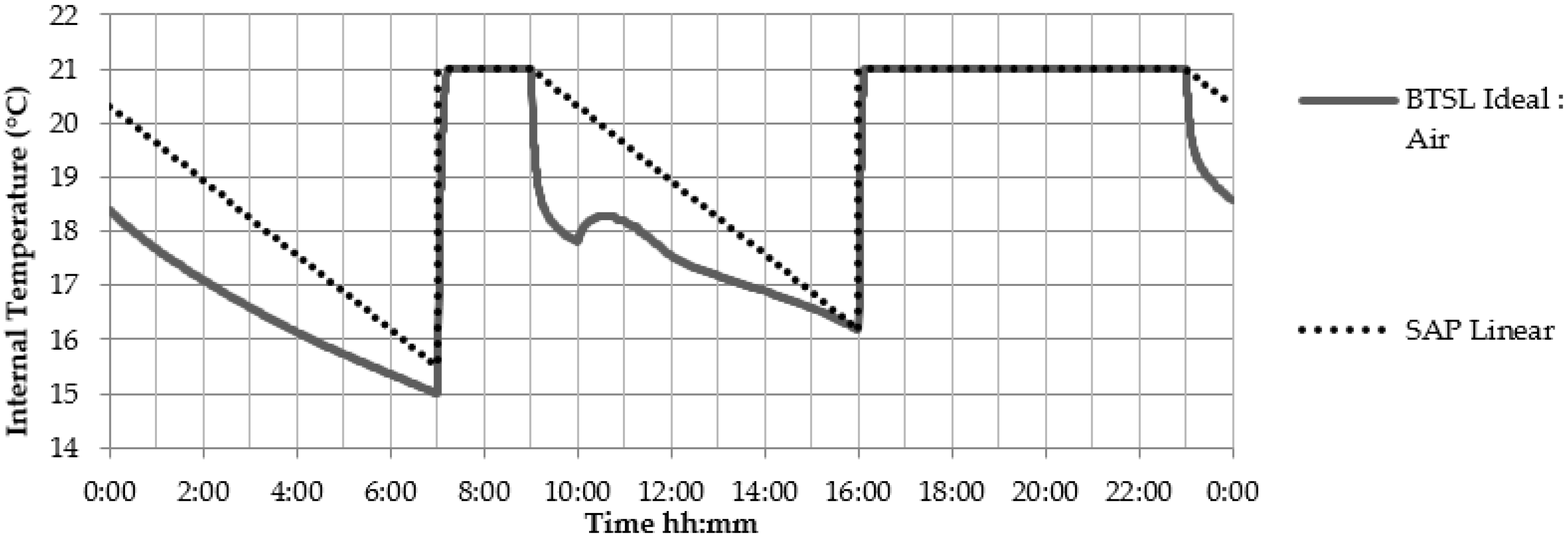
Outside of the heating-on period the mean temperature during the cool down of the building is calculated based on the building fabric parameters of HLP and TMP. A resulting time-temperature profile can be seen in Figure 4 (labelled “SAP Linear”) for the specific case under examination in this paper. Finally, the floor area (Z1 and Z2) and time-weighted combination of internal temperatures during both heating-on and heating-off phases gives the monthly MIT for the heat loss calculation. In this way the intermittency of the heating system is addressed by modelling continuous heating to a lower set-point temperature.
2.1.2. BTSL: TRNSYS and Simulink
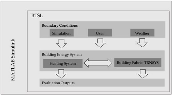
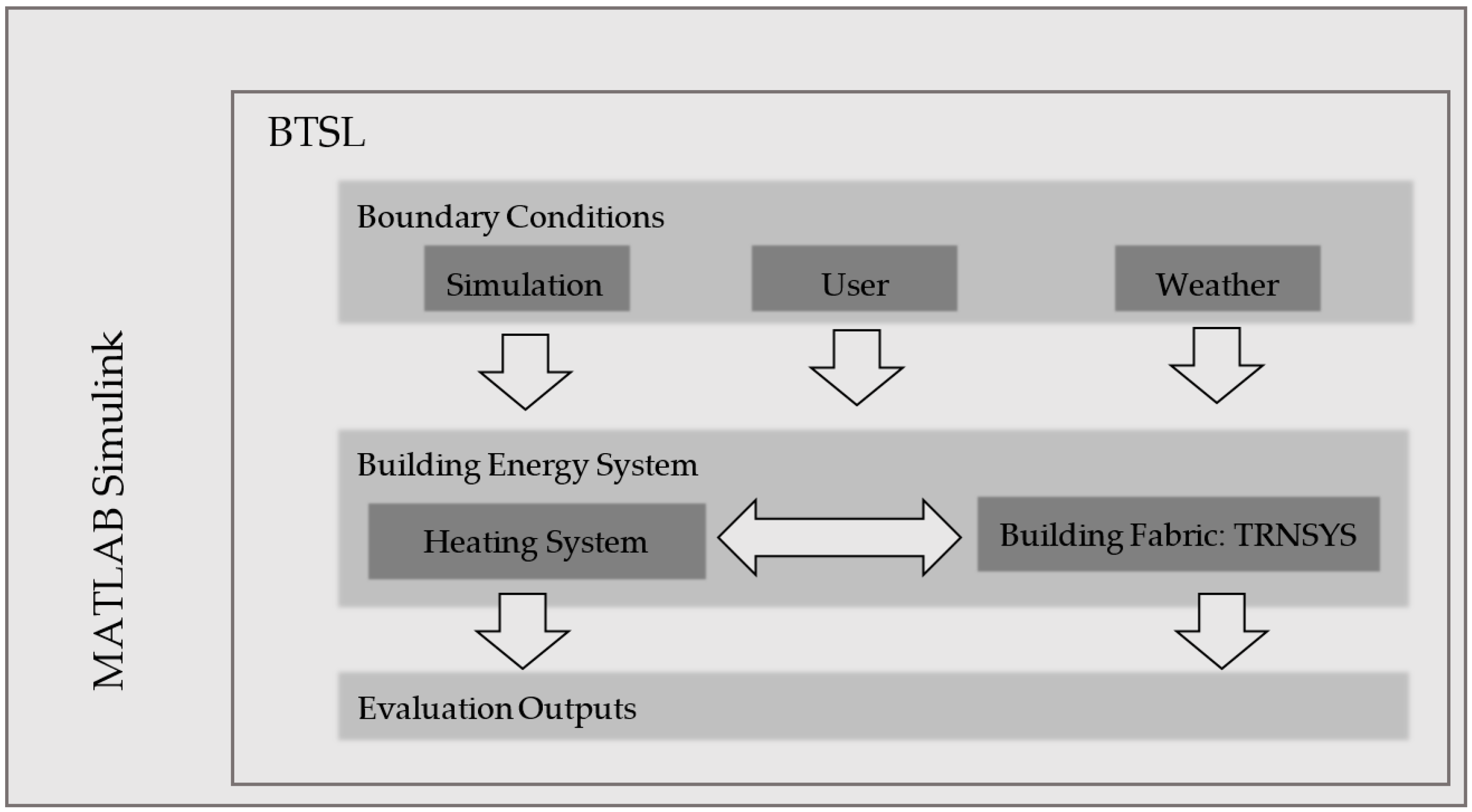
The BTSL model is a fully dynamic engineering model with a library of simulation blocks such as archetypes of buildings and users, which can be linked within the MATLAB Simulink environment, the interaction of these elements is shown in
Figure 1. MATLAB [
23] is a software package for modelling, simulating, and analysing linear and non-linear dynamic systems in continuous or discrete time-steps. Simulink is a sub environment of MATLAB, which uses the MATLAB coding system, allowing the block-based models to be edited and arranged graphically.
The origin of BTSL is from a proprietary heating system emulation tool for product development at Bosch Thermotechnology called Labhouse [
24,
25] (which has since developed and expanded into the current BTSL library and includes a wide range of HVAC components such as radiators, thermostatic valves, boilers, cooling coils, fans and pumps). BTSL is designed to support the development of heating systems and thus has a high level of flexibility with regards to the heating system library block in SIMULINK but uses an existing building model, TRNSYS [
26], to simulate the building fabric. The TRNSYS building model, known as “Type 56”, is a modular transient system simulation program, which meets the general technical requirements of the European Directive on the Energy Performance of Buildings making TRNSYS a potential candidate for compliance with the directive’s implementations in various EU countries. Simulink has an open architecture that facilitates linking models developed in different programming languages, such as C, Java or FORTRAN, therefore enabling TRNSYS 5 Zone Type 56 building model to be implemented into the BTSL library, alongside the proprietary heating system blocks of Bosch Thermotechnology. The hierarchies of these various models and programming environments are shown in
Figure 1.
The advantages of engineering models include the ability to simulate new technologies and their interactions [
21], detailed understanding of energy flows and temperatures. However, engineering models depend on detailed input information about technical performance of the building components and technologies, occupant behaviour and unspecified end-uses leading to potentially erroneous results [
27], which can be exacerbated by the increasing number of input parameters [
28].
The BTSL model allows for modular creation of a building model, whereby the heating system and building characteristics, user behaviour and weather can be varied. The advantage over other available models is the depth of detail at which a user can specify the heating system. Individual system components, such as pumps, pipes and valves can be included, parameterised and physically modelled. In addition the transient behaviour of the heating appliance is modelled through time response parametrization, control feedback loops and the associated control algorithms. This type of proprietary modular concept is used in industry to simulate heating systems under a number of installation environments and verify behaviour and control strategies. An analogous modular construction of simulation in the MATLAB environment with a TRNSYS Building model has been suggested by Rysanek and Choudhary [
29] which served the purpose of evaluating the possible intervention options, building and HVAC system, available in a building upgrade situation.
2.2. Test Case
The basis for the comparison will be a SAP calculation for a sample house, which contains both input and output data from a variety of buildings with a wide range of heating systems. The chosen test case is a detached two-storey house with an above average standard of efficiency (C80 rated EPC). The input data used for both the SAP and BTSL models is summarized in
Table 1, full data is available as
Supplementary Materials to this paper.
Differences between SAP and the resulting BTSL model result primarily from the additional complexity of the latter model to support a more detailed and dynamic simulation of the dwelling, requiring a higher number of input parameters, such as the heating system components and full internal/external wall construction materials and dimensions. It was necessary to make assumptions to provide BTSL parameters in cases where no data was required in SAP, for example the properties of internal walls, and thickness and layers in the building fabric.
A BTSL user behaviour profile was created, aligned to the calculation method of the SAP and is specific for the building under consideration due to inter parameter dependencies, such as the number of inhabitants being proportional to the building floor area. This user profile contains the heating schedule and setpoint temperatures, as well as the metabolic, electrical and hot water heat gains; internal gains were all matched according to
Table 2.
The dynamic BTSL model requires daily external temperature profiles, rather than the monthly averages used in SAP; a weather data file from the US Department of Energy was used [
30], the location of which was chosen to best replicate the location of the test case building, in this case at Finningley, UK. The annual average heating season external temperature difference between that assumed by SAP and the Simulink weather file is <0.7 K (for heating season, SAP 6.81 °C, BTSL 6.18 °C). Additionally, because SAP uses only the outdoor air temperature to calculate the heat loss to the environment, whereas BTSL uses also the ground temperature for the loss through the ground floor and basement, the Simulink model was altered to link the air and ground temperature, so that the air temperature was used as the external temperature regardless of the external surface type.
Zone setup in SAP is differently implemented in BTSL due to the 5 Zone structure of the building model therefore Zone 1 is matched by size and location since this is the living space and leading in the consideration of comfort and space heating. Zones 2 to 5 were set at the same temperature in BTSL.
Since SAP assumes an instant response to heating, BTSL was run firstly with an “ideal heating” system to allow direct comparison, i.e., heat input to the building zones without a normally defined heating system, where heat is delivered through a zero thermal mass active layer in the building virtual fabric. In this way the heat input will exactly and instantly match the requirement of the building, up to a limit of 3.5 kW per zone, resulting in a near instantaneous rise of internal air temperature to achieve the set-point.
2.3. Parameter Space
Following the ideal heating base case a series of representative heating systems were introduced into the BTSL model to investigate the theoretical impact of different heating system parameters. A wet radiator gas fired boiler system was modelled, with thermostatic radiator valves and utilising a system parameterised with laboratory data from the manufacturer Bosch: a Greenstar iJunior boiler [
31], since replaced by the Greenstar i [
32] both of which include the same main heat exchanger.
The parameter space under investigation in the BTSL model covers the variables related to the heating system that are assumed to have no influence on MIT in SAP and is summarised in
Table 3. In the case of heating controls SAP considers that having no control or basic controls will affect the MIT (not considered in this research), otherwise more sophisticated controls are considered to improve the efficiency. This study includes heat up optimisation, a common function on heating system controls, which aims to achieve set point temperature by the specified programmer time; the user can expect the room to be at the desired temperature when the heating period starts, therefore, eliminating any delay due to the responsiveness of the heating system or time response because of the building thermal mass. The simulated control types all are comparable to the SAP test case description of “Room Thermostat”, i.e., the variables altered in BTSL as shown in
Table 3 do not alter the calculated SAP temperature or energy from that used in the base case.
The heating period under consideration in the investigation was October to April, although SAP considers the heating period to last from October to May. May was excluded from the comparison to help focus on the winter heating response and thereby focus on the differences in heating system modelling and not on transient response during the transitional months. For the simulated example building the heating was only required for a few days in May and the overall contribution to the annual space-heating requirement is less than 3%. A more detailed analysis of the winter-to-summer transition periods with regards to dynamic effects could be the subject of further investigation.
MIT is used by SAP as a key determinant of the overall space-heating requirement of the building, therefore, this parameter is calculated from the dynamic simulations for comparison with SAP predictions of MIT. More detailed time-based plots of the internal temperatures were made in order to understand the possible reasons for any differences relative to the SAP benchmark. Furthermore, the space-heating requirement of the building was also calculated from the heat flow from the boiler entering the heating circuit therefore bypassing issues of boiler efficiency, which are not considered in this analysis. The space heating serves as a secondary way of verifying the difference between the simplified EPC/SAP model and the more complex BTSL.
3. Results
For the ideal heating system BTSL obtains similar results to SAP, within 0.2 °C and 200 kWh. Such small differences between the results are expected due to the differences in assumptions and input parameters between SAP and BTSL, in particular the difference in mean external temperature (SAP external temperature is 0.7 °C warmer than BTSL) and how internal walls and external walls construction materials and dimensions, are specified, as discussed in
Section 2.2.
Having verified that the ideal heating system BTSL and SAP return similar results, a physically realistic gas boiler heating system with thermal capacity in the boiler and radiators was introduced, as described above. The results of this investigation and comparison to BTSL ideal heating case are discussed below.
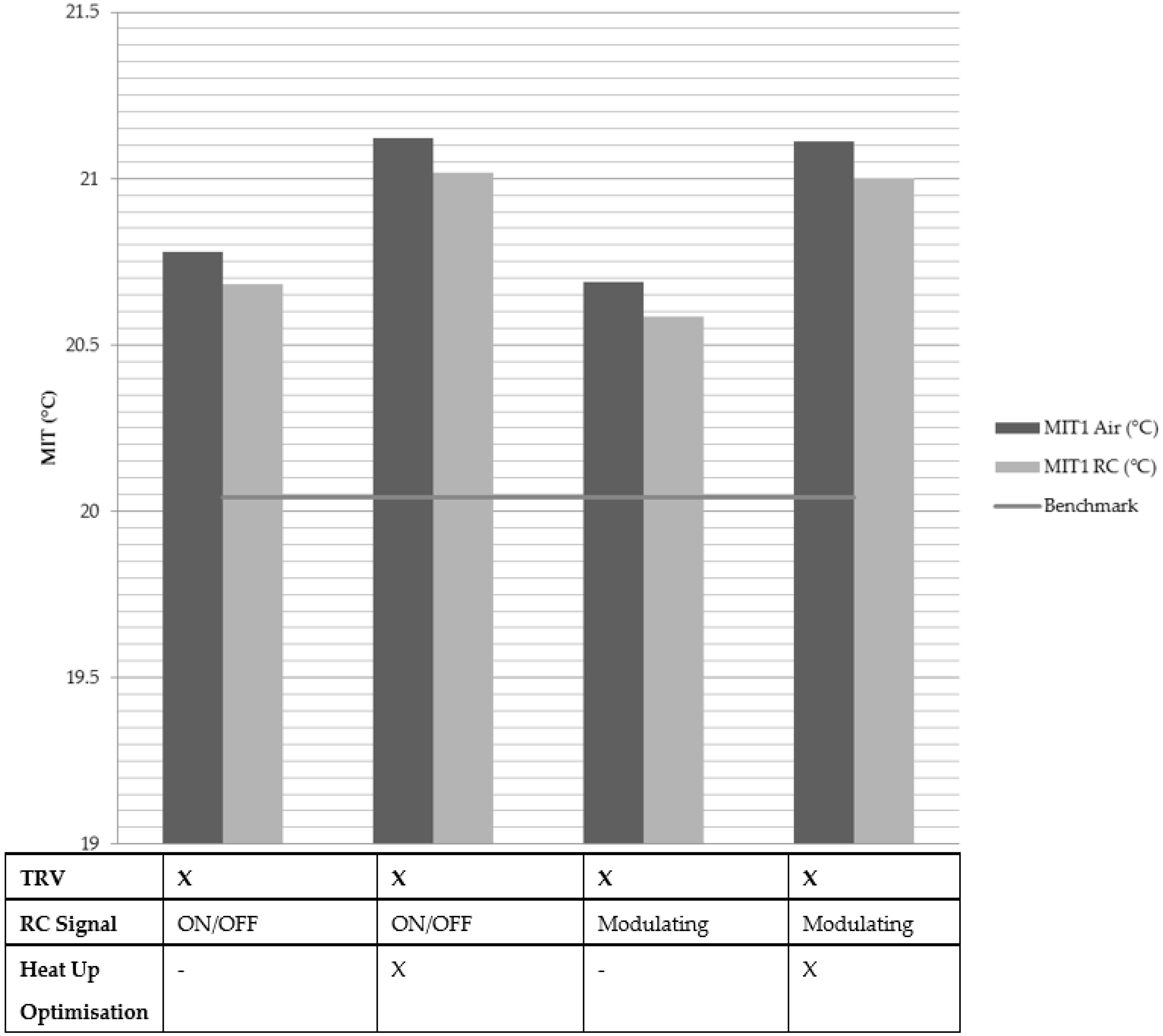
3.1. Heating System Control
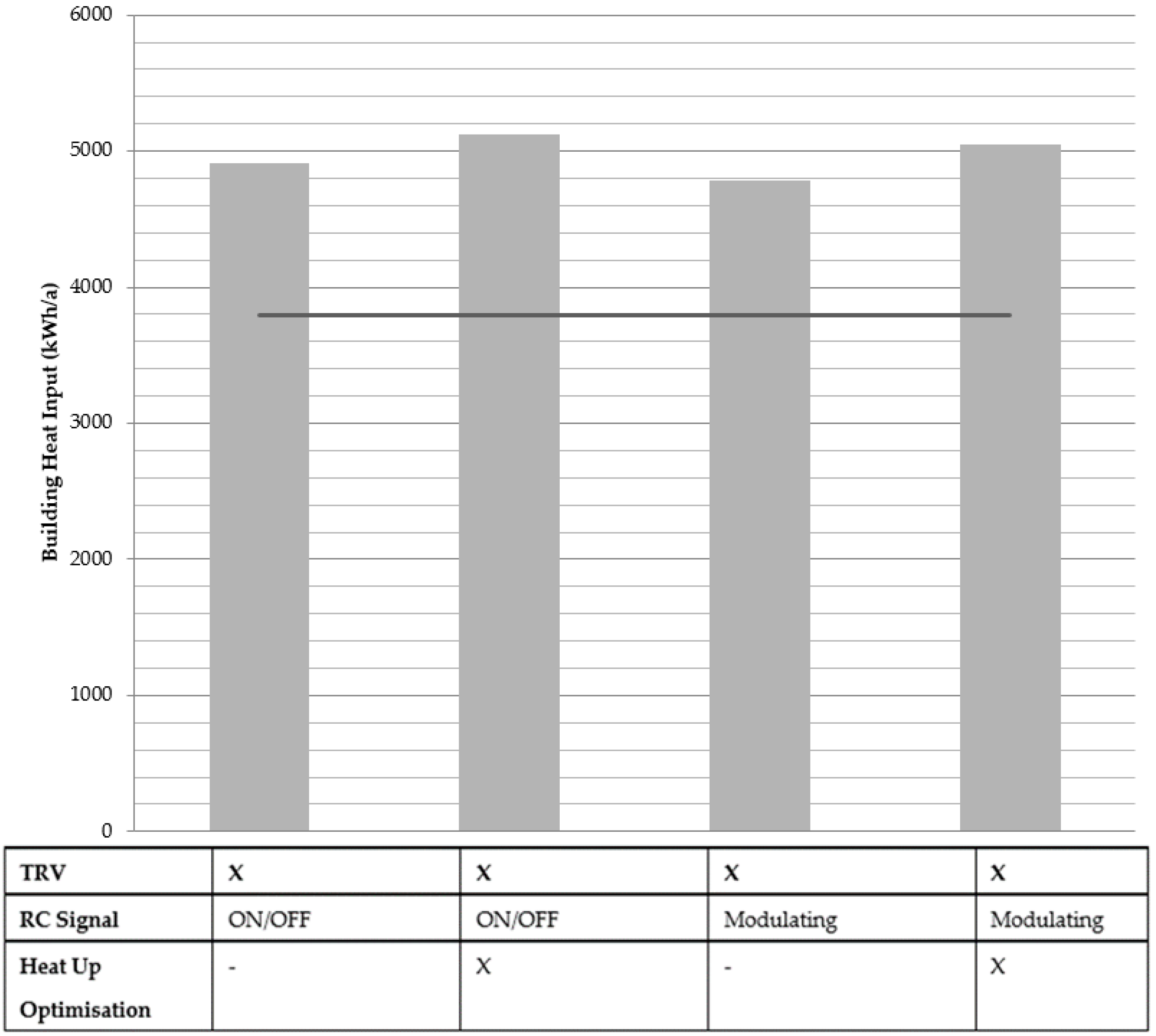
Figure 2 shows two columns for each simulated heating system scenario; representing the air temperature at the central node of each zone (Air) as well as the temperature used by the Room Controller (RC) for feedback. RC and air temperatures differ because the former is influenced by the temperature of the wall on which it would be fitted in order to more accurately measure the operative temperature felt by the inhabitants; in this case the influence is modelled with a ratio of 75/25 Wall/Air based on RC measurements of typical Bosch products [
34], compared to the more typical 50/50. Murphy [
14] noted that SAP does not specify whether operative or air temperature is controlled, and it is often assumed to be the mean air temperature, this could be classified as a type of convention error [
28] or definitional uncertainty [
35]. However, in this analysis both temperatures have been plotted for clarity.
Figure 2 and
Figure 3 shows that all BTSL model results simulating heating systems with thermal mass result in higher MIT and space heating energy demand than predicted by SAP. As above, we note that SAP utilises a 0.7 °C higher external temperature than the BSTL model, which is expected to raise MIT and reduce energy demand in the former model. The variation within the BTSL simulations shows up to 0.5 °C and a 300 kWh/a variation. The two BTSL calculations with the lowest MIT and space heating requirement are the cases without heat up optimisation (which aims to achieve set point temperature by the start of the programmer period); the modulating thermostat shows the lower result.
The internal temperature plots shown in
Figure 4,
Figure 5,
Figure 6 and
Figure 7 represent the Zone 1 conditions across two days in early January and allow closer investigation of the dynamic effects.
Figure 4 shows that BTSL ideal heating achieves a near instantaneous heating up of the building air and perfect control of the setpoint temperature, reflecting a dynamic interpretation of the SAP model assumptions. Murphy [
14] developed a dynamic model implementation of SAP and observed a similar cool down profile to that observed here in the BTSL ideal heating case; similar to SAP the physical detail of the thermal mass of radiators and heating water was not included in Murphy’s study.
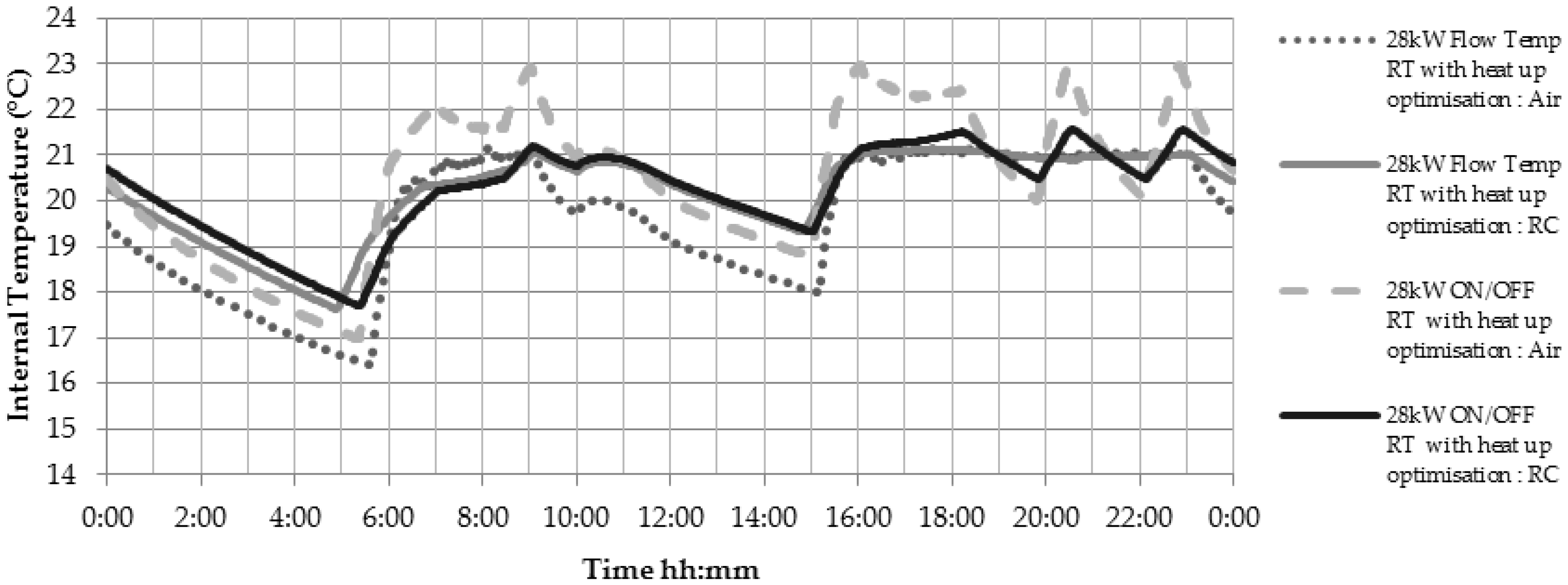
Figure 6 and
Figure 7 illustrate the temperature overshoot of a simple ON/OFF control compared to control, which modulates the flow temperature of the space heating water. All simulations from the BTSL model including the physically realistic heating system exhibit a slower internal temperature decay than that derived in the absence of this heating system. With a physically realistic heating system the property, therefore, has a higher room temperature at the start of each heating period. Given that the building fabric remains the same throughout all the simulations, the addition of the heating system, with its associated thermal storage, is likely to be responsible for this slower temperature decay, through the delivery of residual heat at the end of the heating period.
Air temperature is consistently higher than the RC (wall influenced) temperature in
Figure 6 and
Figure 7. This is to be expected because RC contains a proportion of wall temperature, which is lower than air temperature. An additional feature of note is the increase in internal temperature shown in all situations between 09:00 and 12:00, this is directly related to the solar gain and the east facing orientation of the majority of the windows.
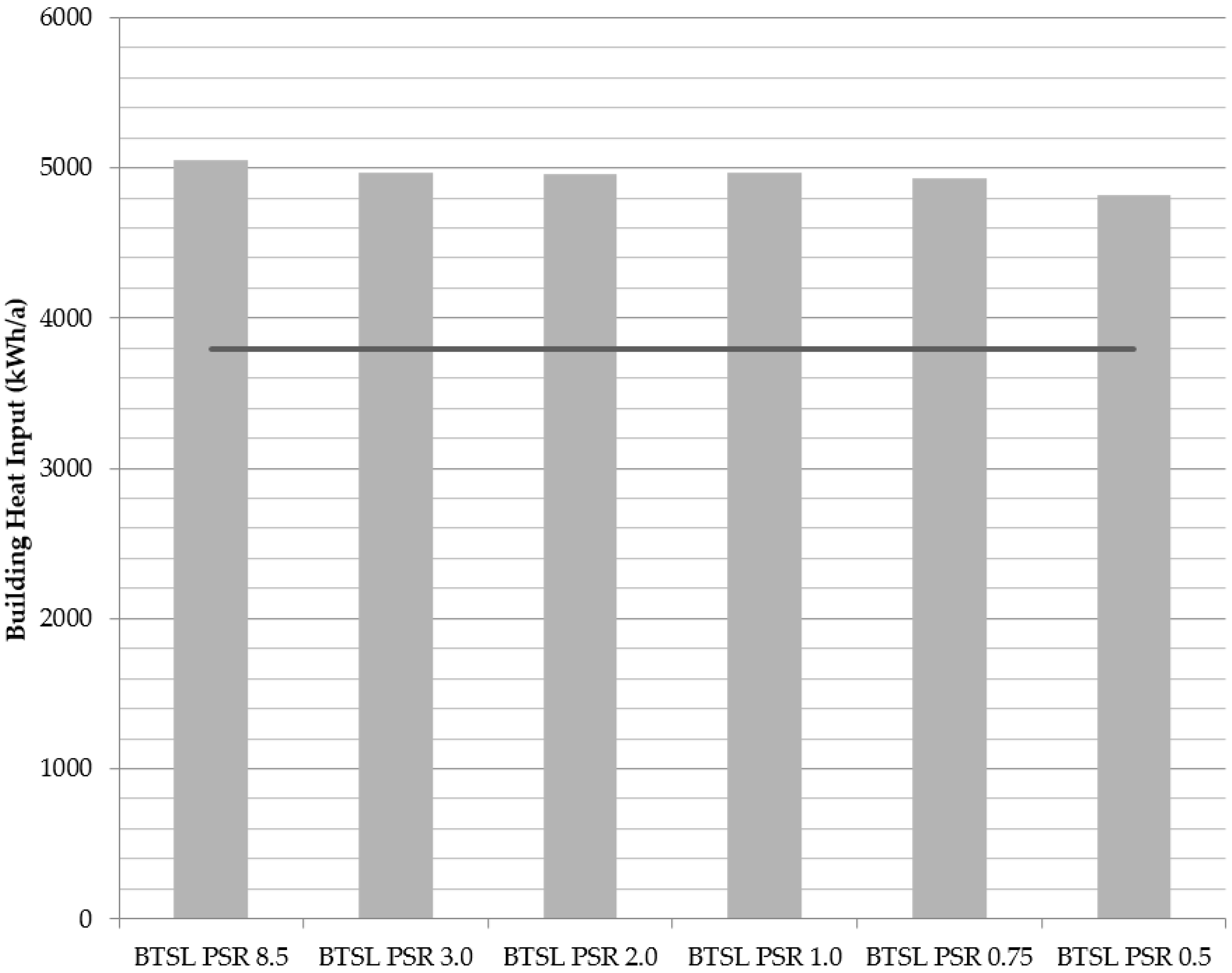
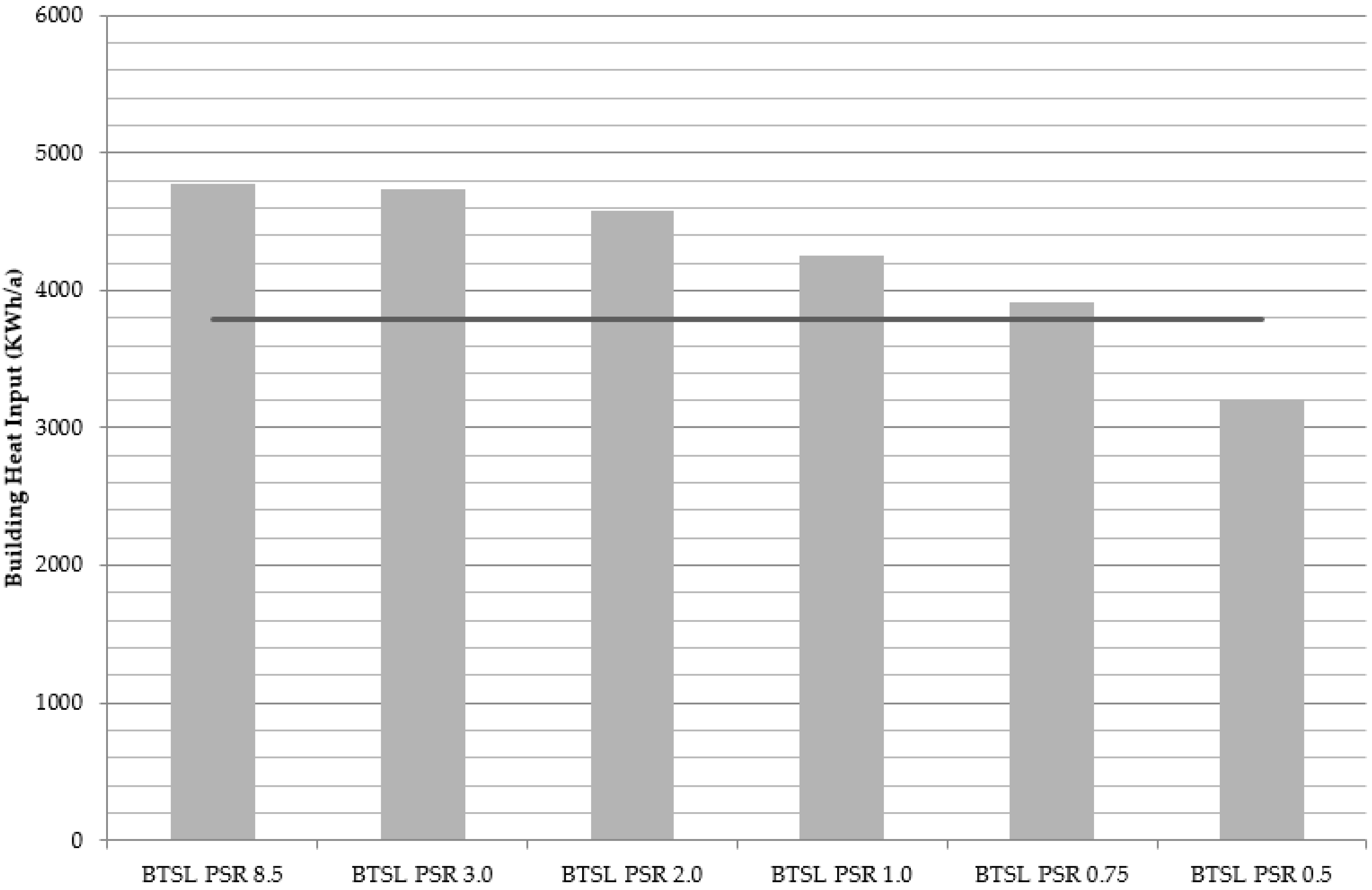
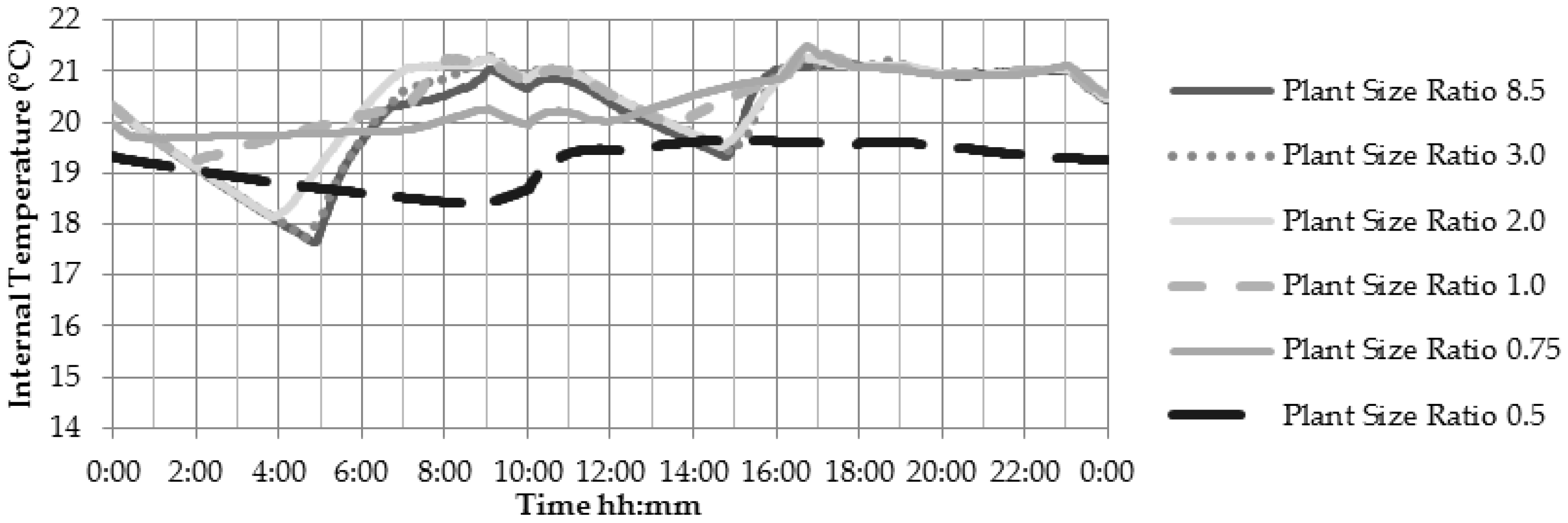
3.2. Plant Size Ratio
In addition to the various heating control types simulated, the Plant Size Ratio (PSR) was also varied from a maximum of 8.5, which corresponds, in the house modelled here, to a common combi boiler output size of maximum 28 kW, down to 0.5 (1.7 kW Boiler Output) whereby the heating system is half the size it needs to be to heat the house when the outdoor temperature is −2 °C. The BTSL combi boiler simulates a typical modulation range of a modern condensing boiler [
31], whereby the ratio of maximum heat output to minimum output was 6:1 meaning that the lowest available heat output of the boiler increased with PSR.
The heating system size was calculated using a design day temperature of −2 °C, whereby the desired internal setpoint temperature can be maintained under continuous and steady state operation of the heating system. However, the practicality of choosing a boiler from a product range based on finite kW output steps will inevitably lead to oversizing of the heating system. This tendency for oversizing was noted as long ago as 1977 [
36] and has been researched both in the UK by the Energy Saving Trust [
37], and in Germany by Fraunhofer Institute [
38]. Oversizing of heating systems is exacerbated in the case of combination appliances since the power output to provide hot water on demand often far exceeds that of the space heating, leading to little correlation between building heat load and boiler size [
37]. Research shows that the oversizing is prevalent and a contributing factor to heating system underperformance [
37,
38]—though we note that in principle, oversizing can lead to improved performance, because of the reduced temperature drops across oversized heat exchangers, if also fitted.
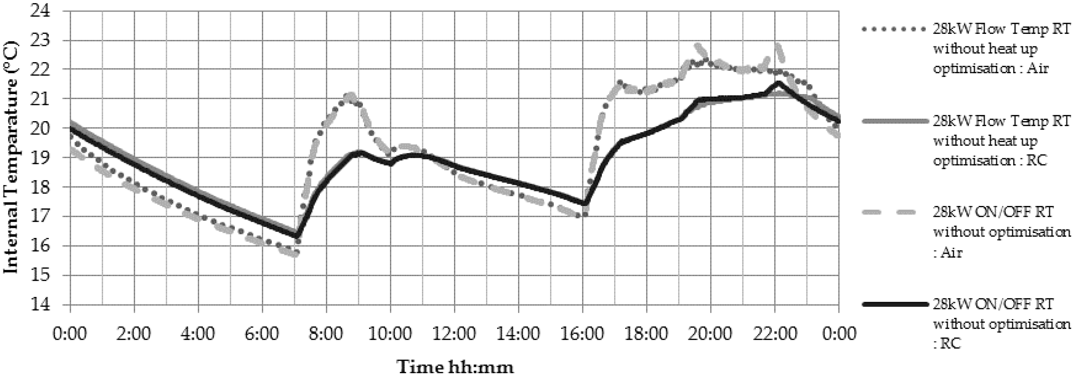
When the “Heat up Optimisation” is disabled in the BTSL model the heating system is restricted to operation during the programmed heating schedule. With this setup the effect of PSR is bigger, see
Figure 7, oversized heating systems exhibit higher MIT than the ideal case and undersized significantly lower. PSR of 1 predicts an MIT close to that of the ideal and SAP case and PSR 0.75 is close to matching the heat input requirements, as shown in
Figure 8.
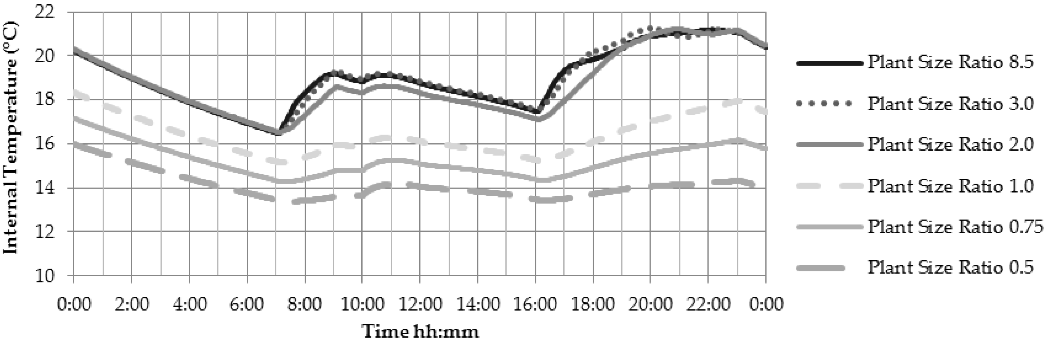
However, a closer inspection of the internal temperatures in
Figure 9 shows that a PSR of 1 gives internal temperatures below the setpoint temperature. This failure to meet the set-point temperature consistently throughout the day occurs despite an average MIT over the heating season which matches that of the SAP and BTSL ideal prediction. During the longer evening heating period the systems with PSR higher than 1 have enough time to reach the setpoint temperature, but with a delay of over 3 h. This would probably be undesirable from the point of view of a real dwelling inhabitant and may lead to changes in the heating program or other adaptations in order to achieve the desired internal temperatures.
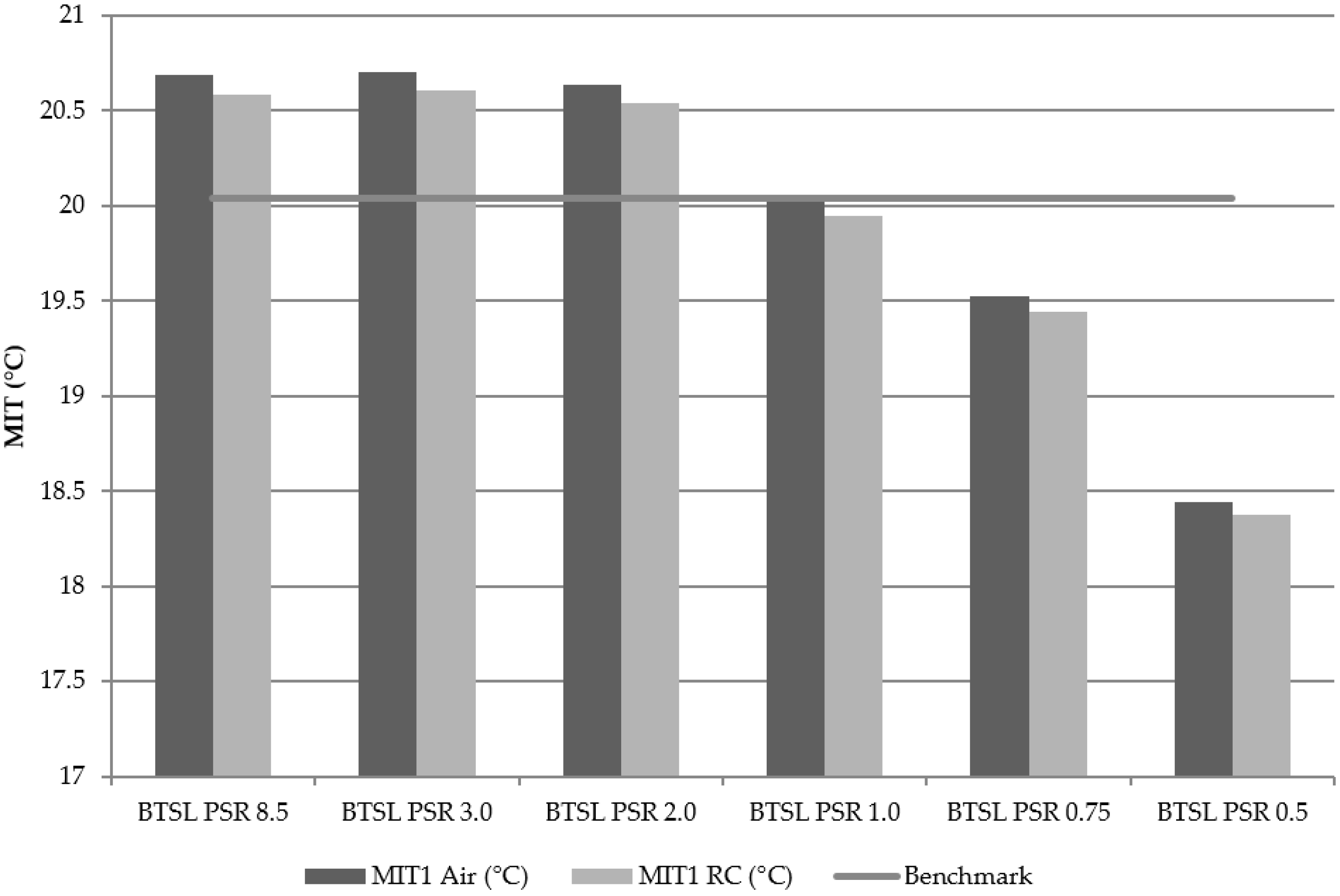
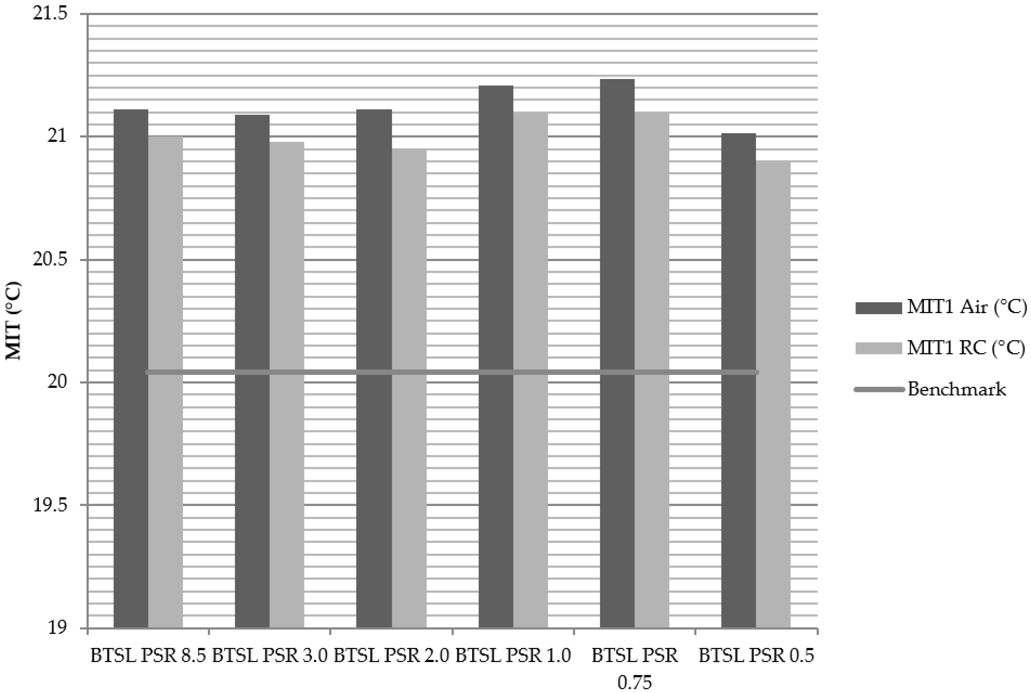
Varying PSR and using the “heat up optimization”, all dynamic BTSL cases resulted in higher MIT and space heating (
Figure 10) than the SAP benchmark. Similarly, the trends in space heating energy are shown in
Figure 11.
The predicted internal temperature profiles (
Figure 12) show that the PSR at which the desired internal temperature, in each heating period, is not reached lies between 1 and 0.75 in the cold month of January. Such PSR can still achieve internal setpoint because the design outdoor temperature is −2 °C, whereas average external temperature in the weather data is 4.6 °C. In the case of PSR 0.75, the temperature was only reached and maintained when the heating period was over 2 h and the previous off period was 7 h during daytime. If the heating schedule had been inline with German norms then it is probable that the variation of PSR would have an effect similar to that of the “heat up optimization” case shown here, since the schedule in Germany consists of only two heating periods, day and night setback. Only in the case of 0.5 PSR was the setpoint unable to be reached during any of the heating periods, with a corresponding drop in space heating energy use. Considering the cases as a whole, there is a tendency for more continuous operation with decreasing PSR, which could be influential when moving away from housing stock dominated by gas heating to less oversized heating systems, such as electric heat pumps, more weather compensated control types or even a shift towards German style heating schedules.
4. Conclusions
Building energy models cannot be expected to capture the full complexity of real building and system performance, in practice useful and useable models must be developed with explicit consideration of which elements to omit to ensure the desired balance of accuracy, reliability and user practicality. The design of NCMs is also subject to this trade-off as demonstrated by Gratzl-Michlmair et al. [
39] when comparing the non-domestic NCMs of Germany and Austria where increased input detail did not result in significantly different predictions.
By transferring a dwelling model from the quasi-static steady state environment of SAP into a dynamic simulation model such as BTSL the effects of not only a basic heating system but also variations in control type and plant size ratio were investigated. The results indicate that there is a significant gap between the mean internal temperature predicted by SAP and that of the dynamic cases; between 0.6 °C and 1.2 °C for a normally sized heating system in this case study. This is expected to be caused by the effect of residual heat in the heating circuit, which is then transferred to the dwelling outside of the programmed heating period, an effect that is not captured by SAP. Inclusion of such a phenomena in the NCM would have a significant impact on the ability of an EPC to distinguish between different heating system and installation types therefore better informing decision makers. It could be possible to implement these effects into the methodology of SAP through a scalable addition to the building thermal mass based on typical heating system design, which would then store heat in proportion to the design setpoint temperature of the heating system as opposed to the setpoint of the dwelling air.
Variation in heating control type and plant size ratio also influences the internal temperature and energy. Poor feedback mechanisms result in temperature overshoot of 1 °C adding controlled feedback improves the situation, reducing error to 0.1 °C, with the best performance being shown by feedback coupled with modulation of the boiler output temperature. Variation of the plant size ratio showed that following guidelines to install PSR approaching 1 may result in internal setpoint temperatures not being met in winter without the use of heat up optimization algorithms, which allow the heating system to operate outside of the programmed heating period, or intervention from the occupier. It is likely that most boilers are oversized, however the heat emitters may be undersized, particularly in older properties or when radiators may not be fully filled with water and require “bleeding”.
This paper has clearly demonstrated that significant differences occur in EPC calculations if more realistic heating systems are modelled by including thermal capacity of the heating system and heating system size. Some of the performance gap between modelled and measured energy performance may be due to both these factors and that the simplifications in the UK SAP method may wrongly give preferential benefit to some heating systems and their controllers. Systems that are likely to be misrepresented include heat pumps, which are typically more closely matched to dwelling heat loss than gas boilers.
There is a clear gap in the theory as implemented in SAP’s quasi-static calculation method relating to heating system specific parameters such as thermal mass, PSR and to a lesser extent control type. Since the BREDEM calculation method is also used for policy evaluation in the UK we believe the simplification may also disadvantage some technologies from a policy context. Improvement of the NCM in this area would lead to a more realistic representation of the relative benefits of different heating systems in EPCs. Sharpening of the near ubiquitous EPCs as a policy tool can help to influence the improvement of domestic heating systems in the UK with respect to efficiency and comfort.
Further investigation into the physical causes for the increased MIT and space-heating requirement of the dynamic situation is required, especially relating to the lower rate of cooling after heating periods. This is expected to be influenced by the thermal mass size, distribution and condition. In addition to further simulations, the behaviour of heating systems measured in situ in buildings would be required to further investigate the magnitude and nature of these transient effects. Further investigation into the method of incorporating such results into the existing SAP framework may then improve its accuracy.
Acknowledgments
This research was made possible by the support of Bosch Thermotechnology Germany with support from the EPSRC Centre for Doctoral Training in Energy Demand (LoLo), grant numbers: EP/L01517X/1 and EP/H009612/1. George Bennett’s PhD is sponsored by Bosch Thermotechnology Germany. Tadj Oreszczyn was funded by Research Councils UK (RCUK) Centre for Energy Epidemiology (EP/K011839/1).
Author Contributions
Cliff Elwell, Robert Lowe and Tadj Oreszczyn conceived the concept of the article and the design of the experimental simulations. George Bennett adapted the model and performed the simulations. All authors analysed the data. George Bennett wrote the paper with support and improvements from all co-authors.
Conflicts of Interest
The funding sponsor, Bosch Thermotechnology, had no role in the design of the study; in the collection, analyses, or interpretation of data; in the writing of the manuscript, and in the decision to publish the results.
Abbreviations
The following abbreviations are used in this manuscript:
| NCM | National Calculation Method |
| SAP | Standard Assessment Procedure |
| EPC | Energy Performance Certificate |
| EPBD | European Performance of Buildings Directive |
| BTSL | Building Technology Simulation Library |
| MIT | Mean Internal Temperature (°C) |
| HLP | Heat Loss Parameter (W/m²K) |
| TFA | Total Floor Area (m²) |
| ACR | effective Air Change Rate (ach, air change per hour) |
| Ψ | Linear thermal transmittance (W/mK) |
| TMP | Thermal Mass Parameter |
| PSR | Plant Size Ratio |
| TRNSYS | Transient System Simulation |
| SEDBUK | Seasonal Efficiency of Domestic Boilers in the UK |
References
- European Commission. Energy Efficiency and Its Contribution to Energy Security and the 2030 Framework for Climate and Energy Policy com(2014) 520 Final; European Commission: Brussels, Belgium, 2014. [Google Scholar]
- EUROSTAT. Final Energy Consumption by Sector (tsdpc320); Eurostat, the Statistical Office of the European Union: Luxembourg, Luxembourg, 2013. [Google Scholar]
- Communities and Local Government. English House Condition Survey; Communities and Local Government Publications: London, UK, 2007.
- Directive 2002/91/ec of the European Parilament and of the Council of 16 December 2002 on the Energy Performance of Buildings; Parliament, E. (Ed.) Official Journal of the European Communities: Luxembourg, Luxembourg, 2002.
- De Wilde, P. The gap between predicted and measured energy performance of buildings: A framework for investigation. Autom. Constr. 2014, 41, 40–49. [Google Scholar] [CrossRef]
- Gupta, R.; Gregg, M. Empirical evaluation of the energy and environmental performance of a sustainably-designed but under-utilised institutional building in the UK. Energy Build. 2016, 128, 68–80. [Google Scholar] [CrossRef]
- Menezes, A.C.; Cripps, A.; Bouchlaghem, D.; Buswell, R. Predicted vs. Actual energy performance of non-domestic buildings: Using post-occupancy evaluation data to reduce the performance gap. Appl. Energy 2012, 97, 355–364. [Google Scholar] [CrossRef] [Green Version]
- Martínez-Molina, A.; Tort-Ausina, I.; Cho, S.; Vivancos, J.-L. Energy efficiency and thermal comfort in historic buildings: A review. Renew. Sustain. Energy Rev. 2016, 61, 70–85. [Google Scholar] [CrossRef]
- Kelly, S.; Crawford-Brown, D.; Pollitt, M.G. Building performance evaluation and certification in the UK: Is sap fit for purpose? Renew. Sustain. Energy Rev. 2012, 16, 6861–6878. [Google Scholar] [CrossRef]
- Majcen, D.; Itard, L.C.M.; Visscher, H. Theoretical vs. Actual energy consumption of labelled dwellings in the netherlands: Discrepancies and policy implications. Energy Policy 2013, 54, 125–136. [Google Scholar] [CrossRef]
- Carmen, G.G.D. Energy efficiency and consumption—The rebound effect—A survey. Energy Policy 2000, 28, 389–401. [Google Scholar]
- BRE. The government’s standard assessment procedure for energy rating of dwellings 2009 edition incorporating rdsap 2009. In SAP 2009; BRE: Watford, UK, 2010. [Google Scholar]
- Hart, J.H.J. BREDEM 2012 Specification; BRE: Watford, UK, 2012. [Google Scholar]
- Murphy, G. Inverse Dynamics Based Energy Assessment and Simulation/Gavin Bruce Murphy; University of Strathclyde: Glasgow, Scotland, 2012. [Google Scholar]
- Wauman, B.; Breesch, H.; Saelens, D. Evaluation of the accuracy of the implementation of dynamic effects in the quasi steady-state calculation method for school buildings. Energy Build. 2013, 65, 173–184. [Google Scholar] [CrossRef]
- Jokisalo, J.; Kurnitski, J. Performance of en iso 13790 utilisation factor heat demand calculation method in a cold climate. Energy Build. 2007, 39, 236–247. [Google Scholar] [CrossRef]
- Corrado, V.; Fabrizio, E. Assessment of building cooling energy need through a quasi-steady state model: Simplified correlation for gain-loss mismatch. Energy Build. 2007, 39, 569–579. [Google Scholar] [CrossRef]
- Deurinck, M.; Saelens, D.; Roels, S. Assessment of the physical part of the temperature takeback for residential retrofits. Energy Build. 2012, 52, 112–121. [Google Scholar] [CrossRef]
- Kim, Y.-J.; Yoon, S.-H.; Park, C.-S. Stochastic comparison between simplified energy calculation and dynamic simulation. Energy Build. 2013, 64, 332–342. [Google Scholar] [CrossRef]
- Kokogiannakis, G.; Strachan, P.; Joe, C. Comparison of the simplified methods of the iso 13790 standard and detailed modelling programs in a regulatory context. J. Build. Perform. Simul. 2008, 1, 209–219. [Google Scholar] [CrossRef] [Green Version]
- Swan, L.G.; Ugursal, V.I. Modeling of end-use energy consumption in the residential sector: A review of modeling techniques. Renew. Sustain. Energy Rev. 2009, 13, 1819–1835. [Google Scholar] [CrossRef]
- BRE. Product Characteristics Database; PCDB: Washington, DC, USA, 2012. [Google Scholar]
- MATLAB. Version 8.2 (r2013b); The MathWorks Inc.: Natick, MA, USA, 2013. [Google Scholar]
- Da Silva, P.; Knabe, G. Labhouse: System simulation and emulation within boiler development. Build. Serv. Eng. Res. Technol. 2003, 24, 281–287. [Google Scholar]
- Perrin, P. Simulationsbasierte Analyse der Einflussfaktoren Auf Betriebszahlen Von Wärmepumpenanlagen; Technischen Universität Carolo-Wilhelmina zu Braunschweig: Braunschweig, Germany, 2012. [Google Scholar]
- Klein, S.A.; Beckman, W.A.; Duffie, J.A. TRNSYS 17: A Transient System Simulation Program; Solar Energy Laboratory, University of Wisconsin: Madison, WI, USA, 2010. [Google Scholar]
- Lomas, K.J.; Eppel, H. Sensitivity analysis techniques for building thermal simulation programs. Energy Build. 1992, 19, 21–44. [Google Scholar] [CrossRef]
- Chapman, J. Data accuracy and model reliability. Available online: http://www.usablebuildings.co.uk/Pages/Unprotected/JakeChapman.pdf (accessed on 8 August 2016).
- Rysanek, A.M.; Choudhary, R. A decoupled whole-building simulation engine for rapid exhaustive search of low-carbon and low-energy building refurbishment options. Build. Environ. 2012, 50, 21–33. [Google Scholar] [CrossRef]
- USDoE. Us Department of Energy Weather Data Files; United States Department of Energy, Ed.; United States Department of Energy: Washington, DC, USA, 2013.
- Worcester, Bosch Group. Installation manual greenstar ijunior 24/28kw. Available online: https://www.worcester-bosch.co.uk/support/document/download/release/8716115166/12640 (accessed on 18 February 2016).
- Worcester, Bosch Group. Installation manual greenstar i 25/30kw. Available online: https://www.worcester-bosch.co.uk/products/boilers/directory/greenstar-i (accessed on 18 February 2016).
- Butcher, K.J. Cibse Guide B-Heating, Ventilating, Air Conditioning and Refrigeration; CIBSE: London, UK, 2005. [Google Scholar]
- Worcester, Bosch Group. Worcester bosch heating controls specifications. Available online: https://www.worcester-bosch.co.uk/professional/support/documents/worcester-controls-specification-document (accessed on 20 April 2016).
- JCGM. International Vocabulary of Metrology–Basic and General Concepts and Associated Terms (Vim 3rd Edition) JCGM 200:2012 (JCGM 200:2008 with Minor Corrections); JCGM: Paris, France, 2008. [Google Scholar]
- Pickup, M. The Performance of Domestic Wet Heating Systems in Contemporary and Future Housing; British Gas Watson House Research Station: London, UK, 1977. [Google Scholar]
- Gastec. Est 2009 Condensing Boiler Field Trial–Final Report; GasTec Enterprises, Inc.: Warminster, PA, USA, 2009. [Google Scholar]
- Wolff, D.; Peter, T.; Budde, J.; Jagnow, K. Felduntersuchung:Betriebsverhalten Von Heizungsanlagen Mit Gas-Brennwertkesseln; Fachhochschule Braunschweig: Wolfenbüttel, Germany, 2004. [Google Scholar]
- Gratzl-Michlmair, M.; Graf, C.; Goerth, A. Vergleichsberechnung eines energieausweises nach deutschen und österreichischen algorithmen. Bauphysik 2012, 34, 286–291. [Google Scholar] [CrossRef]
© 2016 by the authors; licensee MDPI, Basel, Switzerland. This article is an open access article distributed under the terms and conditions of the Creative Commons Attribution (CC-BY) license (http://creativecommons.org/licenses/by/4.0/).


