Daylight Design of Office Buildings: Optimisation of External Solar Shadings by Using Combined Simulation Methods

Abstract

Integrating daylight and energy performance with optimization into the design process has always been a challenge for designers. Most of the building environmental performance simulation tools require a considerable amount of time and iterations for achieving accurate results. Moreover the combination of daylight and energy performances has always been an issue, as different software packages are needed to perform detailed calculations. A simplified method to overcome both issues using recent advances in software integration is explored here. As a case study; the optimization of external shadings in a typical office space in Australia is presented. Results are compared against common solutions adopted as industry standard practices. Visual comfort and energy efficiency are analysed in an integrated approach. The DIVA (Design, Iterate, Validate and Adapt) plug-in for Rhinoceros/Grasshopper software is used as the main tool, given its ability to effectively calculate daylight metrics (using the Radiance/Daysim engine) and energy consumption (using the EnergyPlus engine). The optimization process is carried out parametrically controlling the shadings’ geometries. Genetic Algorithms (GA) embedded in the evolutionary solver Galapagos are adopted in order to achieve close to optimum results by controlling iteration parameters. The optimized result, in comparison with conventional design techniques, reveals significant enhancement of comfort levels and energy efficiency. Benefits and drawbacks of the proposed strategy are then discussed.

1. Introduction

Since the introduction of performance simulation in buildings, several software packages have been developed to cover the different needs of the building industry [1]. Although accuracy and levels of complexity vary among them, most accurate software generally require highly specialized knowledge from users. Moreover, an extended process of trial and error is needed for testing different strategies and obtaining satisfactory results. The integration of parametric design with performance simulation tools has opened new possibilities to overcome these issues by giving the user the ability of testing and comparing and selecting the best possible solution for multi-dimensional problems like the ones found in the built environment.

1.1. Building Performance Simulation: Available Combined Tools

Grasshopper©, is a graphical algorithm editor integrated with Rhinoceros© 3D modelling tools [2]. It allows the modelling of simple and complex geometries, also parametrically controlled. It has gained popularity in the recent years among architects and designers due to its versatility in shape generation. Since its creation, several scripts have been developed, aiming at the integration of simulation tools for different aspects of building performance, such as but not limited to geometry, structures, thermal and daylight performance. One example of these is DIVA, a plug-in for Grasshopper, which stands for “Design, Iterate, Validate and Adapt” [3]. This software allows for environmental analyses in Rhinoceros and its Grasshopper components. It integrates Radiance/Daysim for daylight calculations and EnergyPlus for thermal analyses [4]. Both Daysim and EnergyPlus have been extensively used and validated in research and practice, and their integration in Grasshopper allows them to be accessible to a wider range of users.

Genetic Algorithms (GA) are a particular class of evolutionary algorithms that use techniques inspired by evolutionary biology such as inheritance, mutation, selection, and crossover to evolve a solution for general or specific problems. They have been proven to be an effective strategy for addressing multi-objectives design problems and calculate multiple performance criteria, finding close to optimum solutions in a short period of time [5]. However, their application requires extensive mathematical and computer programming knowledge, far beyond the domain of most professionals. This gap has been recently filled by the creation of Galapagos by David Rutten [6]. The tool is a generic evolutionary solver component available in Grasshopper that integrates GA into a highly intuitive solver. Therefore, different optimization problems can be explored without the need for advanced computing or mathematics skills.

The combination of Galapagos with performative plug-ins could be one of the answers for ensuring high levels of environmental performance while reducing the time needed for extensive trial and error processes. Simulations can be performed automatically and the results stored and organized according to their performance. Thus, rather than setting changes for each simulation, users can set a design problem, and then, obtain the solution optimized for that problem. Alternatively, when a set of multiple good solutions—all meeting the selected screening criteria—are found, professionals can use this collected information as a basis for highly informed decisions. An increase of the environmental performance of new and existing buildings would undoubtedly be the final outcome of this process.

Examples of evolutionary solvers applied in buildings are widely available in the scientific literature. However, due to the complexity of using algorithms to solve design problems, they are generally circumscribed to engineering applications. Uses of GAs can be found for example in the optimization of Heating Ventilation and Air Conditioning (HVAC) control systems for temperature and relative humidity regulation, to deliver high levels of thermal comfort with reduced energy loads [7]. The definition of trade-off between users’ comfort and expenditures (both capital and annual operational) is another example of application of GAs [8]. At the structural level, GAs have been used for the optimization of different structural components of a building. A comprehensive review of different optimization techniques in use to achieve minimum cost, weight, or other specific goals is provided by Sahab [9]. Design of large span structures is the main focus of most of the optimization techniques adopted in structural engineering problems. An example is represented by ParaGen, a parametric modelling and performance simulation software, which integrates genetic algorithms and a database of solutions [10]. This tool, currently under development, was used to optimise the design of large spam roof structures with positive results. Applications for spatial problems have been found for floor layout distribution applied to planning problems [11] or for assigning vertical and horizontal space distribution in large buildings [12]. Regarding acoustic performance, GAs were found in the optimization of noise barriers with variable cross sections [13]. GAs were also found in defining criteria for sizing windows using façade orientation and climatic conditions as dominant parameters [14].

The mentioned studies represent just a few examples in which GAs have been used, in order to optimize the design of one or more building’s sub-systems. However, for most of the cases reported before, the main focus was the solution of a particular problem using specifically developed GAs. In that sense, replicating the proposed logic for different problems would require the development of a new set of specific algorithms and thus, high levels of mathematical knowledge.

Since it has been demonstrated that GAs can play a crucial role in a building’s performance optimization, user friendly tools are needed to expand their use beyond the engineering field.

1.2. Application of Building Performance Simulation to Envelope’s Design: Combining Parametric Design and Evolutionary Optimization

Complex optimization techniques, also involving the use of GAs, have been found to be useful in several problems involving buildings’ envelope designs. Energy and daylight-based optimization functions are usually adopted to find the best solution for a particular design problem.

Trubiano et al. in 2013 [15] developed an evolutionary optimization script, integrating Grasshopper with Radiance and EnergyPlus through Matlab. They used the script to demonstrate the possibility of generating the optimal shape of atriums with the adoption of GAs and a single objective function. A similar approach was used by Lobaccaro et al. [16] for the optimization of the geometry of a building in order to maximise the annual envelope’s exposure to solar radiation.

David et al. [17] applied the combination of daylight and thermal analyses for the assessment of the efficiency of solar shades. They used the shading coefficient, cooling energy demand, daylight autonomy, sun patch index on work plane, and useful daylight illuminance as indexes for rating the performance of different typologies of external overhangs.

Some other research groups have worked on the topic of the optimization of configuration of façade’s modules for office buildings using integrated thermal and lighting simulations. Goia et al. in 2013 [18] carried out the optimization of the window-to-wall ratio of a typical office using total energy consumption as optimization function. They found that, for continental climates (Koppen Geiger Cfb climatic zone), the optimal solution could be obtained for a transparent percentage between 35% and 45%, regardless of the façade’s orientation. Previously, in 2012, Ochoa et al. [19] identified four criteria for the optimization of window’s size in an office building. Together with the minimization of the total yearly energy consumption, they considered illuminance, uniformity, and glare criteria. Instead of defining a univocal solution, they proposed a range of possible solutions, meeting more than one criterion. An open issue was, however, the weight of each criterion in the decision making process. Favoino et al. [20] worked on the definition of an ideal glazed façade for office buildings using thermal transmittance, Solar Heat Gain Coefficient (SHGC) and visible light transmittance as control variables. Also in this case the total primary energy consumption was used as the optimization function.

Since the creation of Galapagos, several researches have explored the implication of this methodology on addressing single or multi objective problems. Although its creator points out that the reliability of the solver depends on the nature and complexity of the studied problem, the results can be better than the ones achieved by traditional approaches.

In 2011, a study performed by El Sheikh & Gerber [21] focused on the parametric design of external shading systems using evolutionary optimization principles. Galapagos was used as the main GA solver, while the optimal solution was searched among the ones able to maximize daylight performance of indoor space. Indicators such as minimum levels of indoor illuminance and luminous distribution of light in the selected space were used.

A similar approach was used by Gadelhak [22] in the form-finding and shading optimization of high performance façades. Similarly to the previous research, daylight indicators such as the percentage of daylit area were used.

Furthermore, the full potential of parametric design integrating simulation tools and genetic optimization using Galapagos has been studied by Shi and Yang [23]. Three simulation software packages were integrated with Grasshopper by writing a customised computer script for each one. Ecotect was used to predict solar radiation availability in complex roof geometry. Radiance was used to define the best window proportion from a given size (height and width) for achieving a specific daylight factor; and EnergyPlus was used for determining the optimal distribution of a given window area for four façades’s orientations (N, S, E and W), with the aim of reducing energy consumption. The research demonstrated that generic evolutionary solvers, such as Galapagos could successfully achieve specific optimization goals. However, two important limitations of the study were pointed out by the authors. Firstly, the studied problems are general and single objectives, whereas, problems in architecture are generally complex and multi-objective. Secondly, coding capabilities are needed to customise computer scripts for integrating different software packages into Grasshopper. This poses a limitation, as designers and architects generally do not have programming skills.

In 2013, Brotas & Rusovan [24] performed an overall energy simulation (including both lighting and energy calculations) of four different envelope solutions for continental climates (simulations were based in London, UK). One of these presented a shading screen previously designed to optimize the daylight performance of internal spaces. The optimization was performed carrying out an evolutionary definition of the shape of hexagonal shadings based on daylight indicators. They found that in such as those climatic conditions, envelope systems adopting optimized shadings could overall achieve better results in terms of CO₂ emissions than traditional solutions.

1.3. Findings from Literature and Aims of Current Research

Overall it can be concluded that the adoption of GA and advanced optimization techniques applied to building envelope design can be highly beneficial. In the selected studies, summarized in the previous paragraph, more accurate solutions than traditional ones were found. Moreover, benefits under visual and thermal comfort viewpoints, as well as substantial energy savings have been predicted.

However, as the literature review indicates, further studies are needed in the area of evolutionary optimization, especially in the development of tools and methodologies that can be used by a wider range of professionals. Explorations on new design methods for integrating parametric design with evolutionary optimization and making use of the existing tools without the need of specific programming knowledge is needed. In addition, the capabilities of generic solvers, such as Galapagos, need to be tested in multi-objective design problems, where the result of one variable has implications on others.

A methodology that integrates the use of genetic algorithms with parametric design for achieving optimised solutions in a highly familiar design software environment is explored here though the combination of the tools mentioned before. The proposed process is tested in a highly recurring design task, such as the optimization of external shadings of office buildings.

2. Materials and Methods

The external shading of a typical office building was set as a case of study, in order to compare traditional design approaches with optimised scenarios. Traditional approaches are defined by experts’ recommendations and by the adoption of deemed-to-satisfy provisions included in energy codes.

Setting external shading as a case study allows for understanding the implication of the shading geometry in both the daylight and thermal performance of the office.

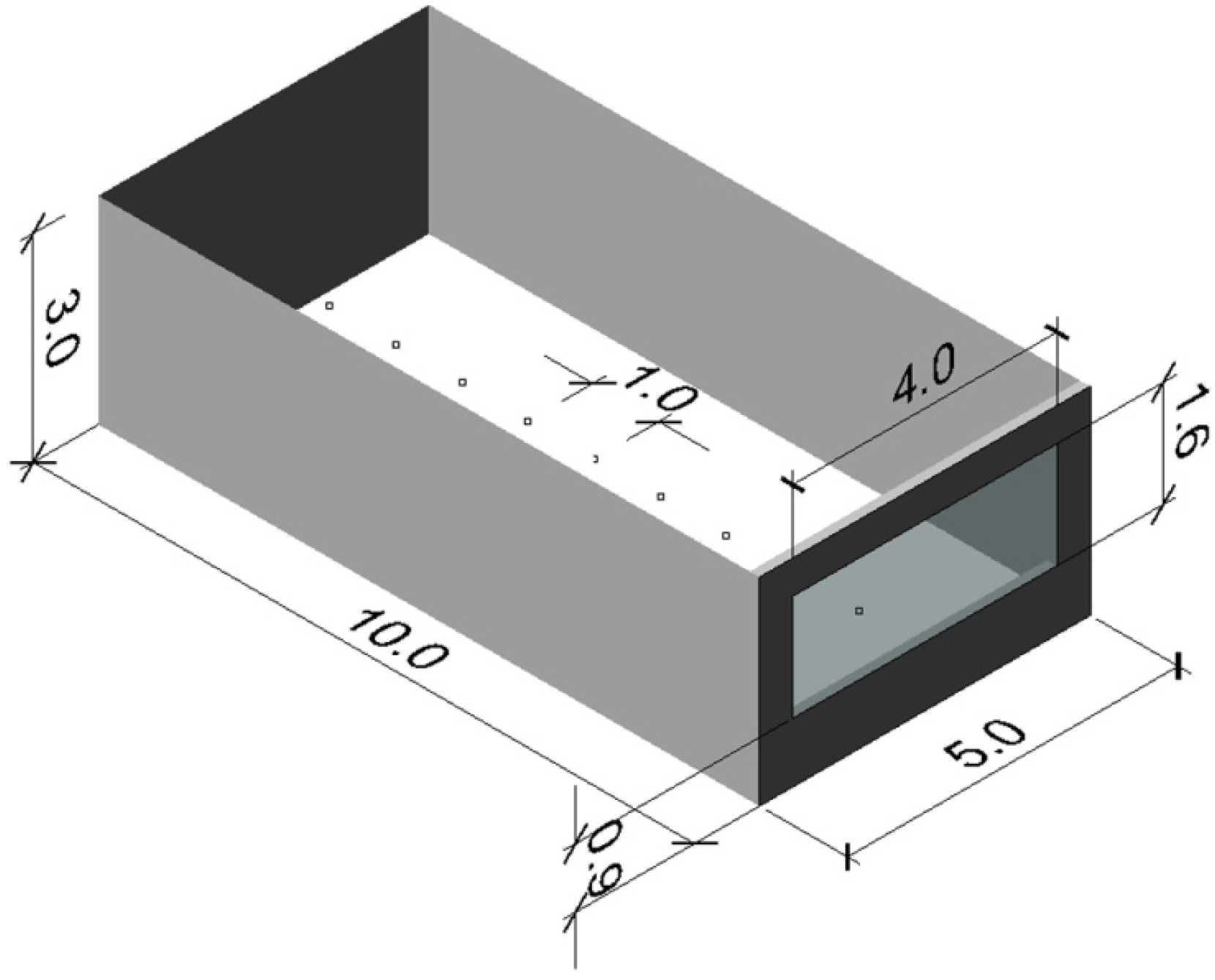
The office is a large rectangular space, with an indoor area of 50 m² and is representative of a multi-user office in large Australian commercial buildings. An overall length of the space of 10 m has been selected, in order to maximize daylight needs typical of open-plan offices. Moreover, the resulting space represents well the case of a perimeter occupied zone of a large-plate (>30 m) multistorey office.

In order to simulate the presence of adjoining spaces, thus considering an office fully included in a whole building, only one wall has been modelled as fully exposed to outdoor. All the other surfaces (back wall, side walls, floor and ceiling) are adiabatic. A geometric representation of the model can be found in Figure 1.

Figure 1. Geometry of the case study and control grid.

Figure 1. Geometry of the case study and control grid.

A north orientation (for the southern hemisphere) of the exposed façade has been chosen in order to maximize issues related to the control of incoming solar radiation. For the same reason, the size of the transparent portion of the wall has been maximized. Except a spandrel portion of 1.6 m (0.9 m below and 0.5 m above the window) and a side portion of 1 m (0.5 m on each side of the window), the wall is modelled as entirely transparent. This results in a window-to-wall ratio of about 43%.

The office has been located in Sydney (New South Wales, Australia, 33°57' S 151°10' E, Koppen-Geiger climatic zone Cfa). The weather file of the Typical Meteorological Year (TMY) for this location has been collected from the database of the United States Department of Energy (DOE).

Properties of building fabric, internal loads, occupancy, and equipment operational schedules are based on minimum standards (deemed-to-satisfy provisions) of the Australian National Construction Code (NCC), section J-energy efficiency [25]. Standards for class 5 (commercial) buildings have been adopted. A detailed list of the provisions is included in the following Table 1.

Table 1. Input parameters for thermal dynamic simulations.

Data	Units of Measure	Value
External wall thermal transmittance (U-value)	W/m2K	0.36
External window thermal transmittance (U-value)	W/m2K	3.80
External window Solar Heat Gain Coefficient (SHGC)	-	0.75
Air infiltration	ACH	1
INTERNAL HEAT GAIN RATE (OCCUPANTS)	W/m2	12
Internal heat gain rate (equipments)	W/m2	15
Artificial lighting power rate (at 320 Lx)	W/ m2	9
Heating set point temperature	°C	20
Cooling set point temperature	°C	24
Heating C.O.P.	-	0.8
Cooling C.O.P.	-	2.5

Table 1. Input parameters for thermal dynamic simulations.

Data	Units of Measure	Value
External wall thermal transmittance (U-value)	W/m2K	0.36
External window thermal transmittance (U-value)	W/m2K	3.80
External window Solar Heat Gain Coefficient (SHGC)	-	0.75
Air infiltration	ACH	1
INTERNAL HEAT GAIN RATE (OCCUPANTS)	W/m2	12
Internal heat gain rate (equipments)	W/m2	15
Artificial lighting power rate (at 320 Lx)	W/ m2	9
Heating set point temperature	°C	20
Cooling set point temperature	°C	24
Heating C.O.P.	-	0.8
Cooling C.O.P.	-	2.5

In order to maximise solar gain, therefore maximizing the need for its control by means of external solar shadings, an ideal clear Double-Glazed Unit (DGU) has been selected as window’s panel. The overall Solar Heat Gain coefficient (SHGC) of 0.75 and a Visible Transmittance of 0.81 reflect the use of two clear 3 mm glasses.

Furthermore, the room has been modelled as fully air-conditioned. Heating and cooling are provided by fan-coil units, and energy is generated by a natural gas boiler and a chiller powered by electricity. Heating and cooling set point temperatures have been defined following currently adopted industry standards in Australian property market [26].

With the aim of simulating the real behaviour of users working in mixed light conditions (i.e., natural and artificial), artificial lighting has been modelled as linearly dimmable and controlled by means of illuminance sensors. Nine sensors, located at 0.8 m above the floor’s level and spaced 1 m each, have been identified. They continuously record horizontal illuminance levels due to natural and artificial light. The combination of natural and artificial light is designed to match a target illuminance value on the workplane of at least 320 Lx across the entire room. This value corresponds to the minimum maintained illuminance required for normal tasks in office buildings in Australia [27].

In order to achieve a good accuracy of daylight modelling results, the following input values have been used for Radiance simulation parameters:

-

Ambient bounces (-ab). This parameter represents the maximum number of diffuse bounces considered. As demonstrated by Mardaljevic [28], -ab values higher than 4 produce high accuracy in results. For the scope of current research, the following previous studies carried out on similar geometries [29] an -ab value of 5 has been adopted.

-

Ambient division (-ad) represents the number of sampling rays projected from each point into the sky for the calculation of indirect radiation. The higher the number, the lower the error in predicting indirect solar radiation. An -ad value of 1024 has been adopted according to [29].

-

Ambient Accuracy (-aa) represents the error—in percentage—of ambient interpolations. An -aa value of 0.1, representative of an error not higher than 10%, has been adopted according to [29].

-

Ambient Supersamples (-as) represent the number of extra rays created between two neighbouring samples when a significant difference (specifically 10% in the current set-up) is found among them. An -as value of 16 has been adopted according to [29].

-

Ambient Resolution (-ar) controls the density of ambient values. An -ar value of 256 has been adopted according to [29].

Table 2 contains materials’ properties used for Radiance daylight models. Materials’ reflectivity and visual transmissivity (i.e., transmission of light at normal incidence) assume the same values for red, green, and blue bandwidths as Daysim scene is simulated in grey colours. In order to consider perfectly diffusive materials, specularity and roughness values of 0 have been used for all opaque materials.

Five different traditional shading settings, grouped in three main scenarios, have been tested. As a base case, an unshaded and unobstructed window has been considered. Then 4 possible shading scenarios have been analysed. The first two involve the use of external multiple metallic louvres sized to shield the window from summer solar rays. The other two represent shading solutions satisfying the requirements of Australian National Construction Code [25] and involving, respectively, the use of an horizontal overhang placed above the window and of multiple external metallic louvres. The 5 traditional settings have been, then, compared with an optimized shading solution, involving the adoption of multiple external metallic louvres. Depth, spacing, and slope of the louvres have been selected as controlled variables for the optimization process.

Table 2. Materials’ properties for daylight simulations.

Building Component	Reflectivity	Visual Transmissivity
Walls and partitions	0.5	-
Ceiling	0.8	-
Floor	0.2	-
Shadings	0.9	-
External ground	0.2	-
Glass	-	0.87

Table 2. Materials’ properties for daylight simulations.

Building Component	Reflectivity	Visual Transmissivity
Walls and partitions	0.5	-
Ceiling	0.8	-
Floor	0.2	-
Shadings	0.9	-
External ground	0.2	-
Glass	-	0.87

2.1. Performance Indicators

Results are then analysed comparing the following indicators:

-

Daylight Autonomy (DA). DA represents the percentage of time in which the indoor illuminance levels at the selected reference point exceed a defined threshold value. For this aim, the value of 320 Lx has been considered as the set point for the calculation of DA.

-

Useful Daylight Illuminance (UDI). UDI is a parameter firstly introduced by Nabil & Mardaljevic in 2005 [30] and accounts for the overall percentage of time during a statistical year in which the indoor illuminance at the selected reference point falls within a defined range. In the current paper, the 4 UDI indicators introduced by Mardalievic et al. in 2012 [31] have been used:

○

UDI fell-short (UDI-f). It represents the occurrence of daylight illuminance levels lower than 100 Lx.

○

UDI supplementary (UDI-s). It represents the occurrence of daylight illuminance levels in the range 100–300 Lx.

○

UDI autonomous (UDI-a). It represents the occurrence of daylight illuminance levels in the range 300–3000 Lx.

○

UDI exceeded (UDI-e). It represents the occurrence of daylight illuminance levels greater than 3000 Lx.

-

Energy consumption for Heating. This indicator accounts for the total energy used yearly on site for feeding the gas heating system and is measured in kWh consumed per year.

-

Energy consumption for Cooling. This indicator accounts for the total energy used yearly on site for feeding the electric cooling system and is measured in kWh consumed per year.

-

Energy consumption for Lighting. This indicator accounts for the total energy used yearly on site for feeding the electric lighting system and is measured in kWh consumed per year.

-

Total Energy Consumption. Sum of the site energy consumed for heating, cooling and artificial lighting.

-

Total Energy Savings. This indicator compares each scenario with the base case on a yearly base.

-

Total CO₂ emissions. This indicator accounts for the total emissions of greenhouse gasses during the process of production of the energy consumed on site for feeding HVAC and lighting systems. The unit of measure is kg of CO₂-e emissions per year. According to [32], emission factors of 0.184 kg CO₂-eq per kWh for natural gas and of 0.86 kg CO₂-eq per kWh for electricity have been used.

Some of the other visual comfort indicators, such as external view and glare probability are here not considered. As a matter of fact the optimized solution, involving the use of external metallic louvres, always offers an obstructed external view. Moreover, as demonstrated in previous researches [33], in the current scenario glare probability is limited.

2.2. Traditional Approaches of Shadings’ Designs

The most basic scenario (no shadings hereafter) is the one in which the external window is not provided with any shading device. The control of solar gains and indoor illuminance levels is simply managed by the transmittance of the glass (in this case fixed throughout all the year). This usually constitutes the starting point of designers for optimizing envelope’s characteristics.

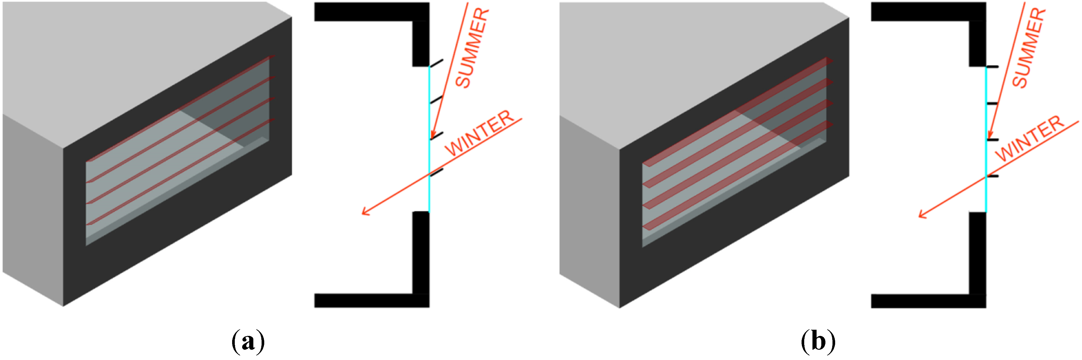
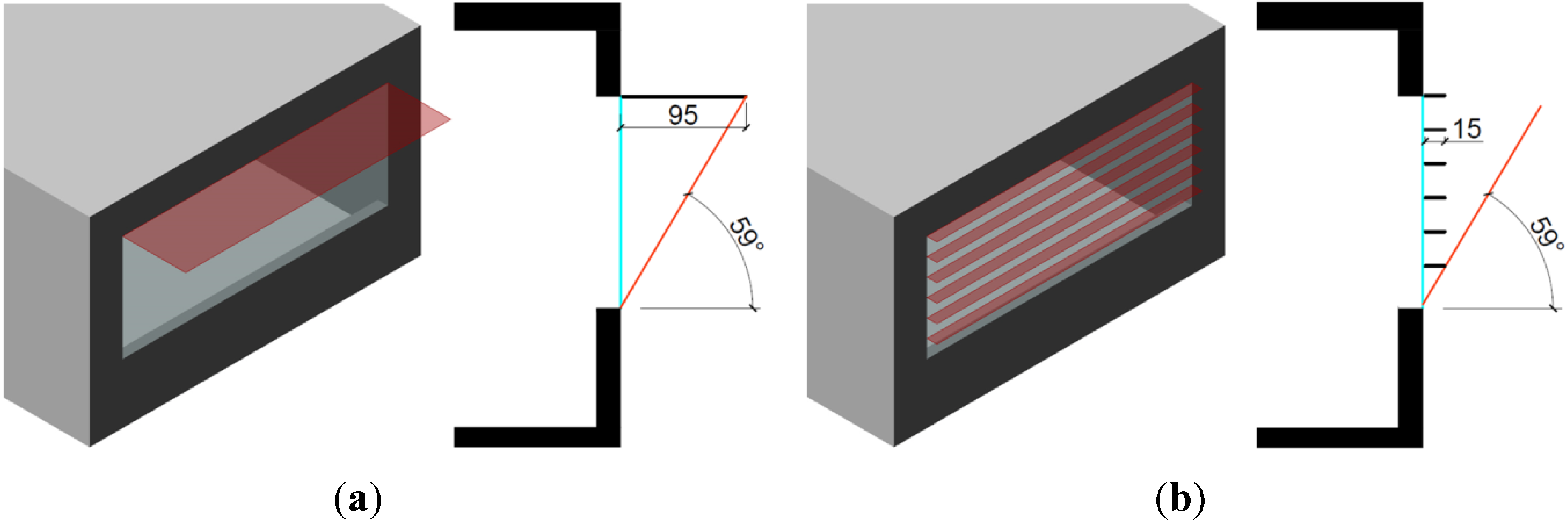
A first improvement is described in Figure 2, where lamellar shadings have been implemented on the external side of the window. Their design follows experts’ recommendations for Sydney’s weather. The base assumption is to avoid solar gains in mid-summer, while gradually allowing them for the rest of the year. This approach is generally adopted by designers who want to go beyond the minimum standard, without engaging with detailed thermal modelling. Two types of shading have been selected. The first one (T1 hereafter) is composed of 4 external lamellas with a width of 150 mm and an inclination of −31° on horizontal plane, allowing a full penetration of winter solar rays and a full blockage of the summer ones. The second type (T2 hereafter) is composed of 4 horizontal louvres with a width of 150 mm. In this case, summer solar rays (calculated at 12 noon of solstice day) are also entirely blocked, with the additional benefit of maximising external views.

Figure 2. Traditional shading regarding building latitude. (a) T1; (b) T2.

Figure 2. Traditional shading regarding building latitude. (a) T1; (b) T2.

The second scenario considers a façade that meets the minimum requirements of the Australian National Construction Code (NCC). The dimension of the shading was defined in accordance with deemed-to-satisfy requirement for transparent surfaces. As a result, a first case (NCC1, thereafter) with an external shading 0.95 m wide added to the upper portion of the window is considered (Figure 3a). The second case (NCC2 thereafter) explores the solution of splitting the external overhang into six horizontal louvres but maintaining the same sun-blocking angle of the NCC1 scenario (Figure 3b). This approach is usually adopted by a designer who wants to maximise daylight through the reflectance of the louvres while still meeting code standards.

Figure 3. (a) Scenario NCC1; (b) scenario NCC2.

Figure 3. (a) Scenario NCC1; (b) scenario NCC2.

2.3. Optimised Shading

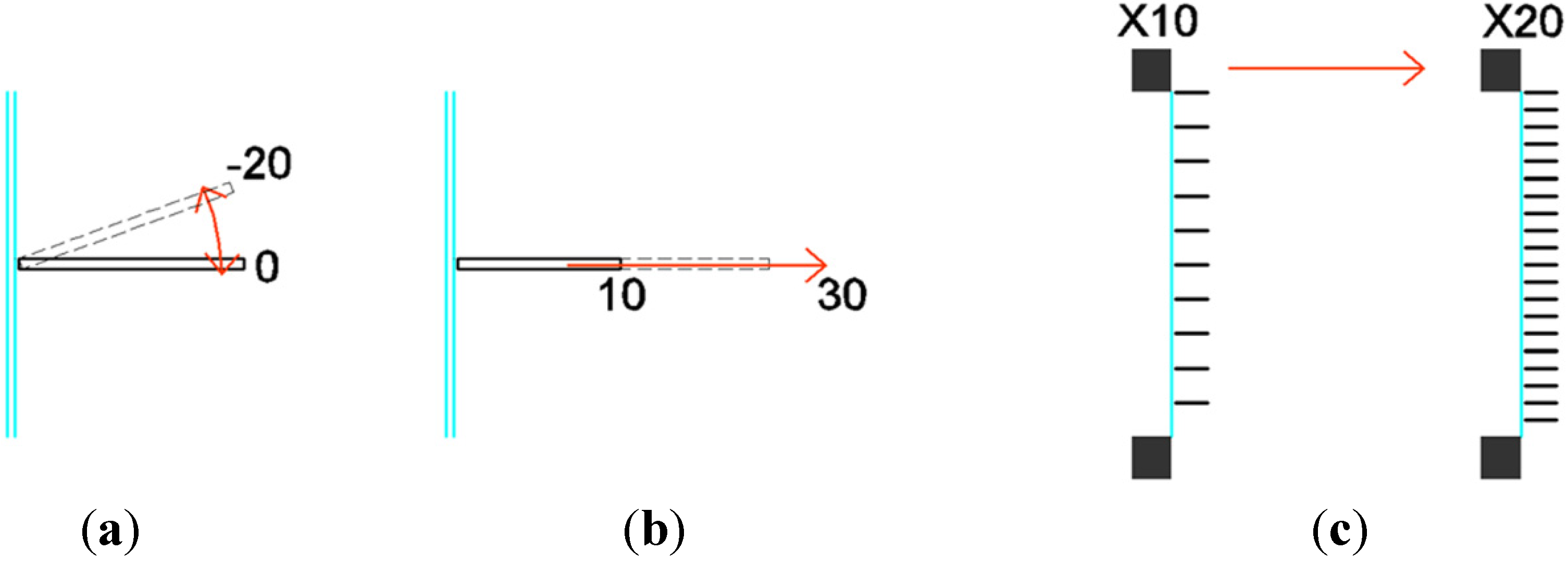
Several variables influence performance of external shading systems and affect both HVAC and lighting energy consumptions. Thus, the optimization of solar shadings is a multi-variable problem. As mentioned before, as the variables cannot be controlled independently, an approach based on GAs for evolutionary optimization has been adopted. The overall geometry of the model has been generated in Rhinoceros and the variation of a limited number of selected variables (genes thereafter) has been managed through Grasshopper. Each gene can assume specific values (genomes thereafter). In the case of the selected optimization, the following genes have been selected. Specific genomes are included in round parenthesis.

-

Shading depth (linearly varying from 0.1 to 0.3 m with a progression of 0.01 m);

-

Shading angle on horizontal plane (linearly varying from −20° to 0° with a progression of 1°);

-

Shading number (positive integer varying from 10 to 20).

The following Figure 4 shows genes and genomes adopted.

Optimization algorithms embedded in Galapagos have been used and total CO₂ emission has been selected as the optimization function (fitness function thereafter).

Figure 4. External shading controllers and function associated: (a) Angle; (b) Depth; (c) Number.

Figure 4. External shading controllers and function associated: (a) Angle; (b) Depth; (c) Number.

The workflow for searching for the optimized solution is summarised in Figure 5. It consists of the following steps:

(a)

Genes are associated with Galapagos (though Grasshopper) that randomly defines a first set of triads of genomes (individuals hereafter).

(b)

DIVA daylight runs the initial daylight calculation based on the first set of individuals. Indoor illuminance levels for each of the 9 sensors are then calculated for every hour of the 365 days of the Typical Meteorological Year. Therefore, the yearly profile of DA is determined for each reference point and, consequently, schedules of artificial lighting are generated.

(c)

DIVA thermal component collects artificial lighting schedule and performs a full yearly thermal dynamic simulation. As a result, final energy consumptions for heating, cooling and artificial lighting are provided.

(d)

Total source CO₂ emissions are calculated, adding components due to heating, cooling and artificial lighting. Total CO₂ emission rate is then defined as the fitness function, and the Genetic Algorithm is set up in order to optimize it (i.e., to find the minimum value).

(e)

The GA solver Galapagos collects and processes the data, commanding the next generation of sets of individuals.

Figure 5. Workflow using DIVA daylight and thermal components, and Galapagos evolutionary solver.

Figure 5. Workflow using DIVA daylight and thermal components, and Galapagos evolutionary solver.

Given the time required for performing daylight calculations, the total search space has been limited to a maximum number of individuals, reducing the number of genomes that each gene could assume. The selection of genomes was based on design constrains, such as the availability of an external unobstructed view and the maximum projection of the shading towards the outside.

The population was set to 10 individuals per generation with an initial population (initial boost) of 20 individuals. Ten percent of individuals passing on at the next generation and a maximum inbreeding factor of 50% insure reasonable variability among generations. Maximum stagnant was set to stop the solver if no improvement of the fitness function was reached after 10 generations. These settings have been defined in order to balance simulation time and accuracy of the optimization process. A similar approach has been previously used by Caldas & Norford [14], Trubiano et al. [15] and Gadelhak [22], adopting respectively 5, 15, and 20 individuals per each generation.

3. Results

The predicted overall annual energy consumption of the typical office in its base case configuration (no shading) is equal to about 2500 kWh, with atmospheric emissions of about 1800 kg CO₂-eq. Adopting traditional shading strategies (T1 and T2), annual overall energy consumptions drop down to about 2000 kWh, and the predicted emissions consequently decrease to about 1400 kg CO₂-eq. These results mostly depend on a substantial decrease of the cooling energy needs due to the reduction of summer solar heat gains. Traditional shading techniques based on solutions compliant to Australian energy code show similar results, with an average overall annual energy consumption of about 1900 kWh and average predicted atmospheric emissions of about 1300 kg CO₂-eq.

The optimization process has been demonstrated to be beneficial in reducing consistently both energy demand and carbon dioxide emissions. Annual energy demand of less than 1600 kWh and annual energy-related atmospheric emissions of less than 1000 kg CO₂-eq have been obtained. Therefore, annual energy savings of about 35%—if compared to the base case scenario—and of 15% if compared to the best non-optimized scenario—have been achieved.

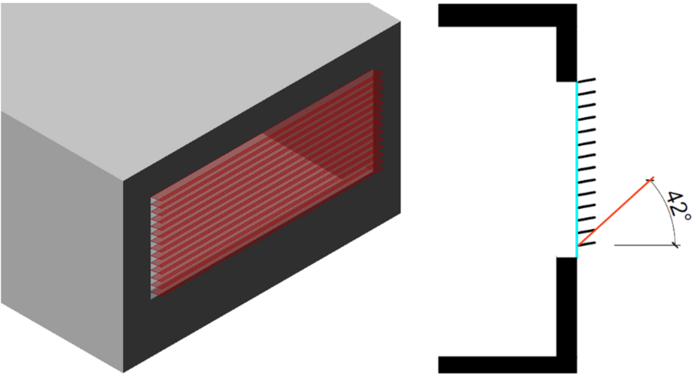
The optimized solution was found with an external system composed of 14 louvres with a slope of −10° on horizontal plane, and a depth of 20 cm (Figure 6). Therefore, the optimized system is able to block completely solar radiation with an incident angle higher than 42°. In addition, the negative inclination of louvres increases the sky view factor of inside points and could potentially increase the reflection of solar rays towards the ceiling. The combination of these two effects could augment daylighting illuminance levels.

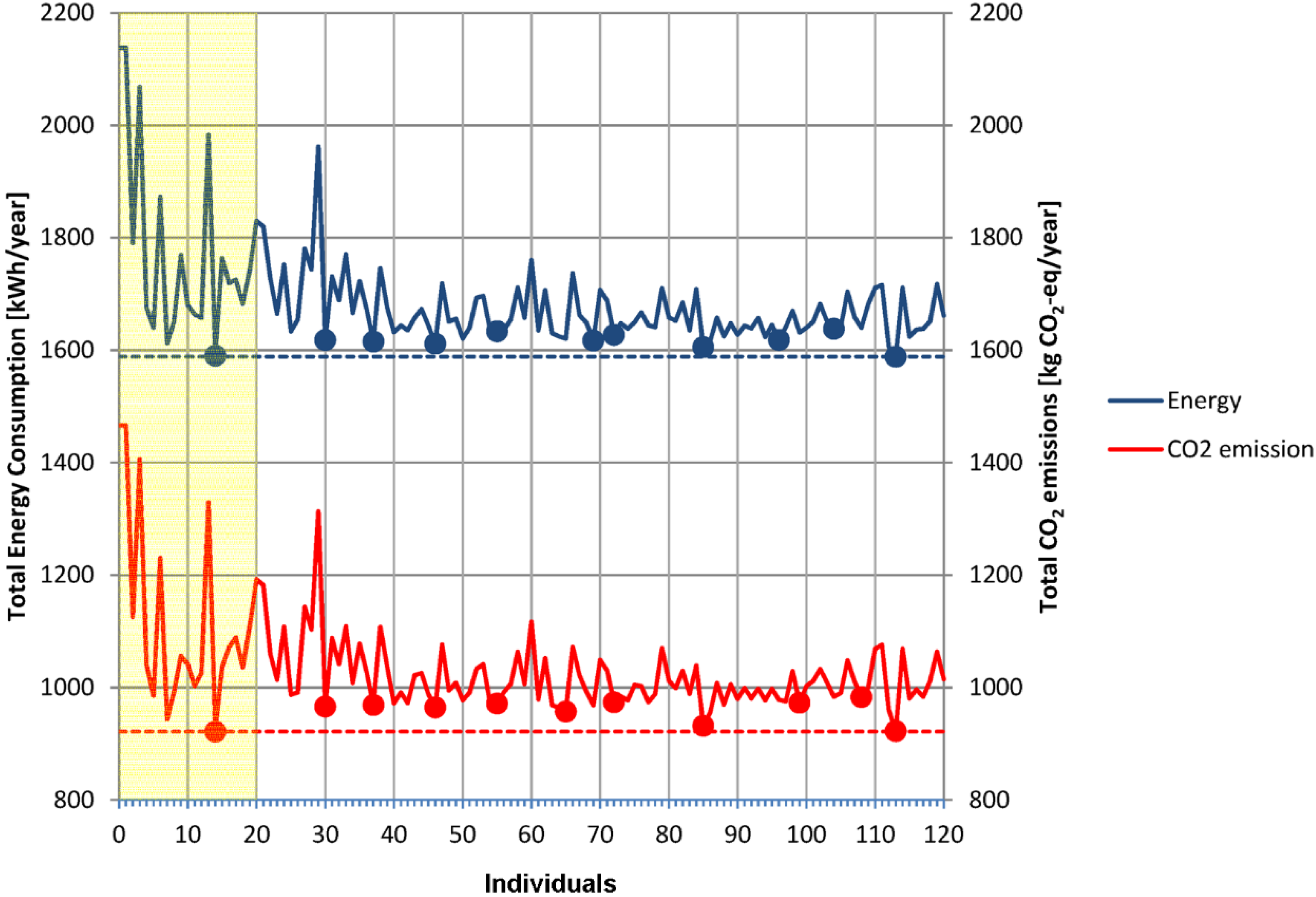
Figure 7 shows the outcomes of the optimization process. The upper curve (in blue) represents the progress in reaching minimum values of energy consumptions after each generation. As can be seen from the figure, a minimum value was already reached within the initial boost (area highlighted in yellow) and was matched in the last generation. The lower curve (in red) represents the progress in reaching minimum values of the fitness function (CO₂ emissions). As can be seen from the picture, in this case, the optimization was also already reached during the initial boost. No better result was found then after the 10 subsequent generations, even though a nearly optimized value was reached in the last generation. For this reason the optimization process was stopped after processing and analysing the 10th generation of values.

Figure 6. Best case scenario.

Figure 6. Best case scenario.

Figure 7. Outcomes of the optimization process.

Figure 7. Outcomes of the optimization process.

3.1. Energy Efficiency and CO₂ Emissions

Table 3 and Table 4 summarise results obtained during the simulation process and compare them in terms of energy consumptions and CO₂ emissions.

As can be noticed from the tables, energy savings increase progressively with the adoption of more sophisticated design techniques. This increase in energy efficiency is mainly due to a substantial reduction of cooling loads (47%, if NCC2 scenario is compared to the base case). Heating and lighting consumptions, on the contrary, do not increase significantly: for the NCC2 scenario, increases of respectively 3.6% and 13.9% were recorded.

As it was demonstrated, avoiding only summer solar radiation (i.e., blocking solar rays sloped more than 75° on horizontal plane) is not a good strategy for offices that generally present high internal heat gains. National Construction Code minimum standards (represented by NCC1) produce good results, avoiding penetration of solar radiation with an angle higher than 59°. However, maintaining the same sun blocking angle but distributing the overhang in a larger number of louvres (NCC2), determines further benefits.

The optimised solution, indeed, experiences significant benefits from the reduction of cooling loads, with a further 47% reduction in comparison to the NCC2 scenario and an overall reduction of 71.9% in comparison to base case. However, due to the reduction of direct solar gains beneficial in the winter period, heating consumption shows an increase of 16.5% in comparison to the NCC2 case and of 20.8% in comparison to base case.

Overall, it can be seen that the optimization process is successful in the reduction of energy consumption, due to the definitions of shading solutions able to better control solar radiation. The contemporaneous reduction of artificial lighting consumption is another proof of this ability.

Table 3. Result summary and comparison for all simulated scenarios. Energy consumption.

Scenario	Shading Setting			Energy Consumptions (kWh/year)				Energy Savings
	Nr.	Angle	Depth	Heating	Cooling	Lighting	Total	(kWh/year)	(%)
No shading	-	-	-	546.33	1458.01	472.73	2477.07	0.00	0.0
T1	4	−31	15	551.28	1205.73	489.68	2246.69	230.38	9.3
T2	4	0	15	559.73	966.05	521.83	2047.61	429.46	17.3
NCC1	1	0	95	556.41	844.27	625.74	2026.42	450.65	18.2
NCC2	6	0	15	566.29	771.32	538.70	1876.30	600.77	24.3
Optimised	14	−10	20	659.73	408.59	521.91	1590.23	886.84	35.8

Table 3. Result summary and comparison for all simulated scenarios. Energy consumption.

Scenario	Shading Setting			Energy Consumptions (kWh/year)				Energy Savings
	Nr.	Angle	Depth	Heating	Cooling	Lighting	Total	(kWh/year)	(%)
No shading	-	-	-	546.33	1458.01	472.73	2477.07	0.00	0.0
T1	4	−31	15	551.28	1205.73	489.68	2246.69	230.38	9.3
T2	4	0	15	559.73	966.05	521.83	2047.61	429.46	17.3
NCC1	1	0	95	556.41	844.27	625.74	2026.42	450.65	18.2
NCC2	6	0	15	566.29	771.32	538.70	1876.30	600.77	24.3
Optimised	14	−10	20	659.73	408.59	521.91	1590.23	886.84	35.8

When it comes to the reduction of CO₂ emissions, the different emission rates for electricity and natural gas slightly change final results. In particular, the CO₂ emission rate for purchased electricity is 4.67 times higher than the one for purchased natural gas. Therefore, cooling and lighting loads have a higher impact on CO₂ emissions than heating loads. As a result, the adoption of optimized external shadings leads to a reduction of annual CO₂ emissions of 47.7%.

Table 4. Results summary and comparison for all simulation scenarios. CO₂ emissions.

Scenario	Shading Setting			CO2 Emissions (kg CO2-eq/year)				Reduction of CO2 Emissions
	Nr.	Angle	Depth	Heating	Cooling	Lighting	Total	(kg CO2-eq/year)	(%)
No shading	-	-	-	100.52	1253.89	406.55	1760.96	0.00	0.0
T1	4	-31	15	101.44	1036.93	421.12	1559.49	201.47	11.4
T2	4	0	15	102.99	830.80	448.77	1382.57	378.39	21.5
NCC1	1	0	95	102.38	726.07	538.14	1366.59	394.37	22.4
NCC2	6	0	15	104.20	663.33	463.28	1230.81	530.15	30.1
Optimised	14	-10	20	121.39	351.39	448.84	921.62	839.34	47.7

Table 4. Results summary and comparison for all simulation scenarios. CO₂ emissions.

Scenario	Shading Setting			CO2 Emissions (kg CO2-eq/year)				Reduction of CO2 Emissions
	Nr.	Angle	Depth	Heating	Cooling	Lighting	Total	(kg CO2-eq/year)	(%)
No shading	-	-	-	100.52	1253.89	406.55	1760.96	0.00	0.0
T1	4	-31	15	101.44	1036.93	421.12	1559.49	201.47	11.4
T2	4	0	15	102.99	830.80	448.77	1382.57	378.39	21.5
NCC1	1	0	95	102.38	726.07	538.14	1366.59	394.37	22.4
NCC2	6	0	15	104.20	663.33	463.28	1230.81	530.15	30.1
Optimised	14	-10	20	121.39	351.39	448.84	921.62	839.34	47.7

3.2. Visual Performance

Results, in terms of selected daylight performance indicators for all the simulated cases are included in Table 5. It can be noticed that for traditional shading techniques (T1 and T2), annual average daylight availability remains almost similar to the one recorded in the base case, with an overall variability of −2%/+1%. The same happens for average, minimum and maximum values of UDI-a. On the contrary, the shading solution compliant with National Construction Code deemed-to-satisfy provisions (NCC1) shows a drop of about 12.2% of the average daylight availability. Interestingly average and maximum UDI-a values do not show a similar pattern (minimum UDI-a decreases of 7.3%, while maximum UDI-a increases of 2.9%). Moreover, for this solution, both UDI-f and UDI-s indicators increase significantly (respectively 6% and 6.3%). The improved solution (NCC2), on the contrary, experiences similar results to the ones obtained of T1 and T2, as it follows similar design principles.

The shading solution resulting from the optimization process determines an increase of useful daylight illuminance levels in the room. In fact, even though DA levels show a decrease in comparison to the base case ones, the percentage of time in which illuminance levels are in a comfortable range increases about 2%, if average values among all nine sensor points are considered. These are the best results among all scenarios.

Table 5. Daylight performance indicators for each tested scenario.

Scenario	Daylight Performance Indicators
	DA (%)	UDI-f (%)	UDI-s (%)	UDI-amin (%)	UDI-aave (%)	UDI-amax (%)	UDI-e (%)
No shading	54.6	17.1	26.3	10.6	44.5	75.8	12.1
T1	55.5	17.4	25.2	8.2	45.5	77.9	11.9
T2	52.7	17.9	27.5	6.5	44.7	81.6	10.0
NCC1	42.4	23.1	32.6	0.7	37.2	78.7	7.1
NCC2	51.8	18.4	27.9	5.4	43.6	81.5	10.1
Optimised	51.4	19.3	27.4	5.3	46.4	81.1	6.8

Table 5. Daylight performance indicators for each tested scenario.

Scenario	Daylight Performance Indicators
	DA (%)	UDI-f (%)	UDI-s (%)	UDI-amin (%)	UDI-aave (%)	UDI-amax (%)	UDI-e (%)
No shading	54.6	17.1	26.3	10.6	44.5	75.8	12.1
T1	55.5	17.4	25.2	8.2	45.5	77.9	11.9
T2	52.7	17.9	27.5	6.5	44.7	81.6	10.0
NCC1	42.4	23.1	32.6	0.7	37.2	78.7	7.1
NCC2	51.8	18.4	27.9	5.4	43.6	81.5	10.1
Optimised	51.4	19.3	27.4	5.3	46.4	81.1	6.8

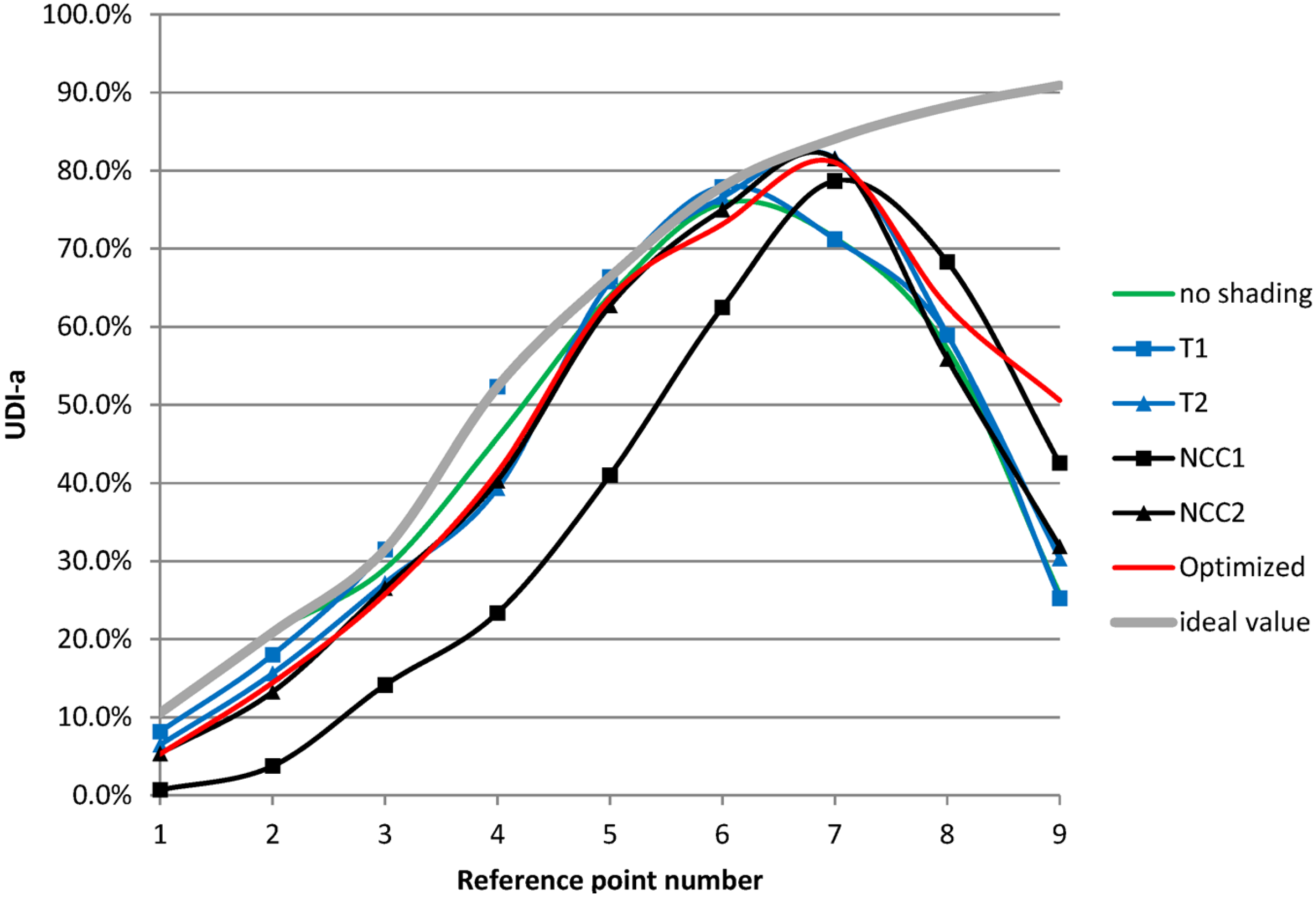
Figure 8 shows the profile of UDI-a for each of the six tested scenarios. Each profile has been calculated considering the nine reference points evenly distributed across the entire depth of the typical office. Ideal values are used as targets for comparisons; they have been defined considering the hypothetical case of a façade system able to clear excessive indoor illuminances (i.e., values over 3000 Lx), while maximising UDI-a percentage.

Base case (i.e., “no shading”), T1, T2, and NCC2 scenarios show similar profiles, with UDI-a values very close to the ideal ones for reference points one to six. UDI-a percentages drop down rapidly for reference points seven to nine close to the window.

Figure 8. Profile of UDI-a for each tested scenario.

Figure 8. Profile of UDI-a for each tested scenario.

In order to explore the benefits of the optimized solutions under a visual viewpoint, horizontal illuminance levels of three selected points have been further analysed. Reference points two (located at 1.5 m from the back wall), five (located in the middle of the room), and eight (located at 1.5 m from the front wall) have been selected as significant for this analysis.

It should be noted that horizontal illuminance values constitute only one of the parameters for the assessment of indoor visual comfort, and more detailed studies should be carried out in the future in order to understand potential glare phenomena associated with the adoption of highly reflective external slats.

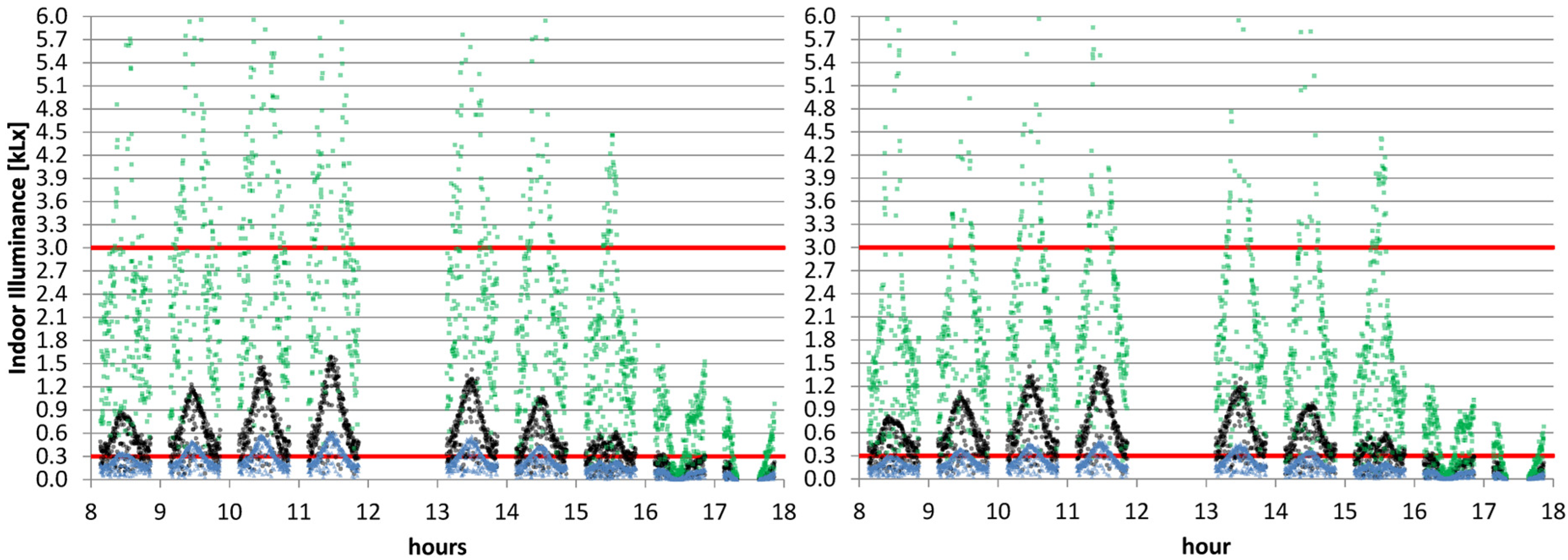
Figure 9 shows the annual distribution of indoor illuminances for the three selected reference points during daily occupancy hours (8 a.m. to 6 p.m.). The two red lines represent the lower and upper limit of UDI-a range. Focusing on the base-case scenario (Figure 9a), illuminance levels at reference point two (blue in the figure) are always lower than 500 Lx; moreover the probability of indoor illuminance levels lower than 300 Lx are high in early morning and late afternoon, especially in winter period. As a result, the annual overall percentage of UDI-a for this reference point is 20.9% and UDI-s contributes for an additional 52.5%. On the contrary, indoor illuminance levels at reference point eight (green in the figure) for about one third of the time exceed the upper threshold of 3000 Lx. On the contrary, in only 7.8% of time, this reference point experiences illuminance levels lower than 100 Lx.

The sensor located in the middle of the room (sensor point five, in black in the figure) experiences more constant illuminance values across all the year. For a wide majority of time (exceeding 85%) users located in this reference point would experience indoor illuminance levels on the workplane in the range between 100 Lx and 3000 Lx. Moreover illuminance levels never exceed the upper threshold of 3000 Lx.

Overall, comparing the distributions of indoor illuminance values of the base case and the optimized scenario, a significant improvement of comfortable horizontal daylight illuminance conditions can be noticed. Sensor points located in the middle and at the back of the room, already experiencing illuminance levels in the comfortable range for the majority of time, also continue to show the same pattern with the adoption of external shadings. Points located close to the window show a substantial increase of the percentage of hours with illuminance levels in the range between 100 and 3000 Lx.

Figure 9. Distribution of indoor illuminance values for sensor points two (blue), five (black), and eight (green): (a) Scenario “no shading”; (b) Optimized scenario.

Figure 9. Distribution of indoor illuminance values for sensor points two (blue), five (black), and eight (green): (a) Scenario “no shading”; (b) Optimized scenario.

4. Discussion

The optimization problem, related to the selection of external shadings in an office building, was solved using an energy-related function (minimization of CO₂ emissions). However, it was found that the specific solution leads to an increase of daylight performances of the spaces. An overall increase of the minimum and average percentage of working hours experiencing comfortable daylight illuminances was found. Moreover, the increase of the uniformity of distribution of daylight illuminances across the entire space was another related advantage. It should be noted that predictions have been made with the assumption that no interior shading device will be needed. However, in some circumstances (for example, in the presence of low sun angles), interior shadings could be needed in order to avoid direct sunlight penetration. This could partially impact lighting energy savings, as well as cooling and heating loads.

Despite the fact that a low number of individuals per generation was used (10 out of 50 recommended), an optimized solution was found. The optimized solution showed a substantial increase of energy performance and environmental sustainability, even if compared to be best “traditional” solution. This, in the authors’ viewpoint, is proof of the utility of the proposed methodology. A similar approach of using a reduced number of individuals per each generation has already been adopted in similar cases [14,15,22] and was found successful. This is a highly beneficial approach when time is a constraint due to the complexity of analyses to be performed. The obtained results are satisfactory, especially considering that Galapagos is an evolutionary solver adopting a generic Genetic Algorithms, which may not be the best optimiser for the specific proposed problem. Considering that each change in the settings affects each component of the energy loads differently, results in a multi-objective problem are difficult to predict. Thus, computer assisted optimization can help designers to solve complex problems in limited time, being that the main advantage of the studied workflow.

In DIVA, the combination of the advanced functionalities of daylight (Radiance/Daysim) and thermal (EnergyPlus) software, allows designer to obtain accurate results. However, each component has limitations that reduce its capabilities on dealing with complex geometries, large areas and/or multiple zones. DIVA thermal component allows the calculation of just one thermal zone per time. Thus, each thermal zone needs to be analysed independently, and the interaction of different zones within a building cannot be assessed. At the same time, this approach unavoidably offers limited possibilities for materials setting. Emissivity is not thermally considered for the shading setting. Thus, the radiation component of the energy emitted by external shadings is not accounted.

Moreover, daylight calculations based on Radiance raytracer algorithms [34] require long simulation time, even for a simple geometry like the studied one. Time required for performing daylight simulations has been demonstrated to be about 35 times longer than the one required for performing a full thermal dynamic analysis. Therefore, the feasibility of conducting an optimization process for large areas or complex geometries is limited, especially when time is a constraint.

Finally, optimized solution may not necessarily be the best solution for meeting other design criteria. In this specific case, parameters as external view factors and glare probability have not been considered. For the optimized scenario for example, negative shading angle and high number of louvres are likely to reduce views towards outside. Therefore, additional criteria need to be incorporated in the problem setting for real applications.

The proposed strategy explores just one component of the building envelope. The same approach or something similar can be used to optimise different design variables of building sub-systems, allowing informed decisions made at different stages of the design process.

It is expected that current limitations of the simulation software tools, in terms of the number of spaces able to be modelled and limited number of design parameters that can be considered, will be overcome in the future. In addition, simulation time is likely to be reduced by the constant evolution of computers processing capacity.

5. Conclusions and Recommendations

In conclusion, this work has demonstrated how:

• The combination of parametric design with evolutionary optimization is a valid strategy for exploring solutions to building environmental performance problems. A comprehensive setting of the design problem and further improvement in the simulation tools could overcome the main difficulties found in this research.
• Solutions optimised by the computational means can differ from traditional ones, providing new answers for design problems that can be more effective on solving specific tested issues. For the studied case, the optimised solution performs significantly better in terms of daylight availability, energy efficiency and CO₂ emissions than other studied alternatives, with different shading configurations.
• Although the methodology was tested for one specific problem that could correspond to an advanced stage of the design process, a similar approach can be used in order to optimise problems such as—but not restricted to—building orientation and geometry, window-to-wall ratio, and thermal resistance of the external envelope.
• Future studies can be built upon the current one and explore an expanded set of optimization criteria, combining energy-related indicator with visual comfort ones, such as glare probability, uniformity of daylight illuminances, and external view factor.