

Adaptive Vibration Monitoring of Railway Track Structures Using the UWFBG by the Identification of Train-Load Patterns


1
China Railway Siyuan Survey and Design Group Co., Ltd., Wuhan 430063, China
2
Hubei Key Laboratory of Track Security Service, Wuhan 430063, China
3
School of Civil Engineering, Harbin Institute of Technology, Harbin 150090, China
4
Key Lab of Smart Prevention and Mitigation of Civil Engineering Disasters of the Ministry of Industry and Information, Harbin Institute of Technology, Harbin 150090, China
*
Author to whom correspondence should be addressed.
Buildings 2024, 14(5), 1239; https://doi.org/10.3390/buildings14051239
Submission received: 8 April 2024
/
Revised: 22 April 2024
/
Accepted: 24 April 2024
/
Published: 26 April 2024
(This article belongs to the Special Issue Recent Developments in Structural Health Monitoring)
Abstract
:Due to the capability of multiplexing thousands of sensors on a single optical cable, ultra-weak fiber Bragg grating (UWFBG) vibration sensing technology has been utilized in monitoring the vibration response of large-scale infrastructures, particularly urban railway tracks, and the volume of the collected monitoring data can be huge with the great number of sensors. Even though the train-induced vibration responses of urban railway tracks constitute the most informative and crucial component, they comprised less than 7% of the total operational period. This is mainly attributed to the temporal sparsity of commuting trains. Consequently, the majority of the stored data consisted of low-informative environmental noise and interference excitation data, leading to an inefficient structural health monitoring (SHM) system. To address this issue, this paper introduced an adaptive monitoring strategy for railway track structures, which is capable of identifying train-load patterns by leveraging deep learning techniques. Inspired by image semantic segmentation, a U-net model with one-dimensional convolution layers (U-net-1D) was developed for the pointwise classification of vibration monitoring data. The proposed model was trained and validated using a dataset obtained from an actual urban railway track in China. Results indicated that the proposed method outperforms the traditional dual-threshold method, achieving an Intersection over Union (IoU) of 94.27% on the segmentation task of the test dataset.
1. Introduction
Urban railway tracks, a pivotal mode of transportation in contemporary urban areas, significantly contribute to the efficiency of transportation and the development of the economy. However, the track structure’s performance may gradually decline due to a combination of factors such as train loads, environmental wear, and material aging [1], and subsequently lead to critical safety risks.
To ensure the safety of train operations, the implementation of structural health monitoring techniques in urban rail transit has become critically important [2,3,4]. Recently, the ultra-weak fiber Bragg grating (UWFBG) sensing system has been developed for large-scale infrastructures due to its capability of multiplexing thousands of sensors on a single optical cable [5,6]. This system has proven to be the ideal monitoring technique for urban rail transit. Despite its effectiveness, the volume of the collected monitoring data surges with the great number of sensors. For instance, a railway track in China, spanning 39 km and equipped with the UWFBG sensing system, accumulates more than 4 TB of data daily. However, due to the temporal sparsity of commuting trains, the stored data predominantly comprise low-information environmental noise and interference signals, while the most crucial data–the train-induced vibration responses under railway tracks–accounts for less than 7% of the total operational period. This underscores the significance of implementing an adaptive monitoring strategy.
To enhance the efficiency of monitoring systems, triggered sampling techniques have traditionally been implemented to initiate and terminate the sampling process via external sensors. This method is well-suited for traditional point sensors operating independently. However, for distributed sensing technologies like UWFBG, applying a uniform start and stop time is impractical due to discrepancies in the times at which each sensor detects the target signal. A potential solution is the development of a data preprocessing algorithm, which is capable of autonomously identifying the segments of the train-induced vibration signals within the monitored data. This ensures the adaptability within the monitoring system.
By formulating the recognition of specific patterns in time series data as a classification problem, traditional methods typically subdivide the signals into smaller segments using sliding windows and classifying each segment based on predefined features. These features may include time-domain features such as short-time energy (STE) and short-time zero crossing rate [7], frequency-domain features like spectral entropy [8] and spectral variance [9], and cepstral features, for instance, Mel-frequency cepstral coefficients [10]. These conventional methods have experienced numerous developments in the field of voice activity detection (VAD) [11,12]. Jiang et al. [13] proposed a dual-threshold method for endpoint detection of speech founded on STE and frequency centroid. The thresholds are determined by the local maxima of the statistical feature sequence histogram. Roy et al. [14] suggested a speech endpoint detection method based on wavelet convolution. This method decomposes the speech signal using wavelet convolution and then automatically identifies speech segments based on thresholds of information entropy in the frequency domain. Ma et al. [15] proposed a speech activity detection algorithm that relies on long-term spectral flatness measurement. Traditional methods have also been found to be applicable in the segmentation of structural monitoring data. Bao et al. [16] introduced an algorithm that combines signal features in both time and frequency domains to recognize intrusion vibration signals in the perimeter security system. Liu et al. [17] enhanced the wavelet thresholding algorithm and the double thresholding algorithm for segmenting traffic flow monitoring data based on distributed acoustic sensing. Among the traditional VAD methods based on predefined features, the dual-threshold method is the most classical and widely utilized method.
However, the accuracy of traditional VAD methods is significantly affected by the effectiveness of the predefined features, and insufficient exploitation often leads to poor accuracy. Moreover, as original signals are processed by sliding windows, the predicted labels are assigned to the entire windows rather than each data point. To overcome these limitations, several researchers have turned to deep learning-based methods. Gaugel et al. [18] proposed a deep learning model that integrates a convolutional neural network (CNN) and a recurrent neural network (RNN) for feature extraction. In this model, the CNN is utilized for intra-window feature extraction, while the RNN is employed for inter-window context detection. However, this method still utilizes non-overlapping sliding windows, preventing it from achieving pointwise segmentation. Perslev et al. [19] introduced a fully convolutional U-net, applying it to the segmentation of sleep electroencephalogram (EEG) data. Londhe et al. [20] proposed a model that employs hybrid channel convolution and a bidirectional LSTM network to extract the temporal correlation of electrocardiogram (ECG) data for time series segmentation. Shang et al. [21] proposed a revised U-net model for segmenting vibration monitoring data of bridges to extract the structural free decay response.
Unlike time-series data such as ECG and EEG, which display more readily identifiable patterns, the vibration monitoring data collected by the UWFBG sensing system pose a unique challenge due to its complexity. Inspired by image semantic segmentation [21,22,23,24,25], this study proposed a U-net model with one-dimensional convolution layers (U-net-1D) for the segmentation of vibration monitoring data. This model does not require predefined features and can achieve pointwise accuracy. Furthermore, a dual-threshold method that integrates STE and a time-frequency domain feature (short-time low-frequency energy, STLFE) is also proposed for comparison. The accuracy and effectiveness of these two methods are validated and compared using the long-term monitoring data collected by the UWFBG sensing system from a 39 km-long railway track in China.
The remainder of this paper is structured as follows: Section 2 introduces the proposed U-net-1D for the segmentation of vibration monitoring data, detailing the loss function used for training and the metrics used for performance evaluation. Section 3 presents the engineering verification of the U-net-1D model and the traditional dual-threshold method, including comparisons between them. Finally, Section 4 concludes this paper.
2. Methodology
In this study, the U-net model is proposed for the semantic segmentation of monitoring data. U-net is a well-established deep neural network architecture and is frequently employed in image semantic segmentation, which involves assigning semantic labels to each pixel and thus facilitates pixel-level classification of the image [22]. U-net has also been widely employed in many fields, such as medical image segmentation [26,27], natural image segmentation [28,29], etc.
2.1. Semantic Segmentation of Monitoring Data
The classic U-net model utilizes 2D convolutional layers to perform semantic segmentation on images. However, when this architecture is applied for segmenting monitoring data, modifications are necessary, including changes to the convolutional layers and activation functions of the output layer. Specifically, in this study, all 2D convolutional layers in the classic U-net model are replaced with 1D convolutional layers to accommodate time series data input. The size of the input layer is modified to match the size of the monitoring data under analysis. Additionally, considering that the prediction labels for the data points in this study are binary (that is, either passing-train signals or other signals), the prediction results can be determined by a single output channel. This channel represents the probability that each input data point is classified as a passing-train signal. Therefore, the output channel of the classic U-net model is reduced to one. The activation function of the output layer is also modified to a sigmoid function, ensuring that the output results fall within the range of (0, 1).
As depicted in Figure 1, the proposed method utilizes U-net-1D to process the track vibration signal and subsequently generates the corresponding point-wise classification probabilities of this signal. The classification probability of the passing-train signal is significantly higher than that of other signals, thereby enabling effective recognition of the trains. In Figure 1, each blue box within the U-net-1D represents a combination of a convolutional layer and an activation layer, whereas each gray box indicates a copy of the feature map. The U-net-1D model is structured with an encoder on the left and a decoder on the right, each comprising four sequential 1D convolutional blocks that form the core architecture of the model. The encoder serves as a contracting path that performs down-sampling through max-pooling layers, with both the pooling region width and stride set at 2, thereby halving the size of the feature map. In contrast, the decoder acts as a symmetric expanding path that executes up-sampling through transposed convolutional layers with a stride of 2, which doubles the size of the feature map. To facilitate the integration of feature maps of varying depths from the encoder, skip connections, indicated by gray arrows, are implemented between the encoder and the decoder. ReLU activation functions are employed in all layers except for the output layer, which uses a sigmoid function. N denotes the length of the input signals.
2.2. Weighted Loss Function
The loss function based on cross-entropy is extensively employed in tasks involving semantic segmentation, as it effectively quantifies the disparity between the predicted probability distribution and the actual label distribution [30]. In the case of segmentation with only two class labels, the binary cross-entropy (BCE) is typically adopted and defined as follows:
where and denotes t the true label and the predicted probability of each pixel by the deep neural network model.
BCE is a criterion that computes the mean binary cross-entropy over all data points, leading the segmentation model to weigh each point of the time series uniformly throughout the training process. Nonetheless, it is worth noting that in numerous semantic segmentation applications, there’s often a significant disparity in the volume of data points among various classes. For instance, the passing-train signals typically account for less than 7% of the total monitoring time. This imbalance could lead the model to be biased towards predicting dominant classes, thereby neglecting the minority classes. To tackle this issue, a weighted cross-entropy loss function is usually employed to introduce weights between different data points. Accordingly, the weighted binary cross-entropy (WBCE) is similar to the standard BCE, with the exception that positive data points are weighted by certain coefficients when computing the pointwise loss. The formula for WBCE is as follows:
where denotes the weight allocated to positive data points, which is calculated based on the proportion of negative to positive data points within the dataset under examination. Therefore, in situations where there are fewer positive data points than negative data points, the weight assigned to each positive sample will be greater than 1. This approach ensures that the model pays more attention to the less frequent class during training, thereby mitigating the impact of class imbalance on the model’s performance.
2.3. Evaluation Metrics
In semantic segmentation tasks, Intersection over Union (IoU), Recall, and Precision are commonly used evaluation metrics, which are expressed mathematically in Equations (3)–(5). IoU metric quantifies the overlap extent between the predicted segmentation and the ground truth, determined by dividing the area of their intersection by the area of their union. It evaluates the accuracy of the model in detecting the target, with a higher IoU indicating a greater overlap between the predicted and true results. Recall is a metric that captures the fraction of actual positive instances that the model accurately classifies as positive. A higher Recall indicates a better performance of the model on the positive samples. Precision is the metric that gauges the accuracy of the model in predicting positive instances, calculated as the ratio of true positives to the sum of true and false positives. Elevated Precision reflects a model’s proficiency in minimizing the incidence of false positives. It is worth noting that Precision and Recall are generally in conflict with each other in classification tasks. Improving Precision could lead to a decrease in Recall and vice versa. Therefore, to provide a comprehensive evaluation of the performance of the proposed U-net-1D, these three metrics–IoU, Recall, and Precision–are considered together in this study.
where TP represents the count of true positive samples, indicating the correctly predicted positive instances; FP denotes the false positive samples, referring to the negative instances incorrectly labeled as positive; and FN stands for false negative samples, which are the positive instances that were mistakenly identified as negative.
3. Case Study
An in-situ urban railway track allocated with the UWFBG sensing system in China is employed as the validation in this section. For comparative analysis with the proposed method, a dual-threshold approach that combines STE and STLFE features is also introduced.
3.1. UWFBG-Based Urban Railway Track Vibration Monitoring Data
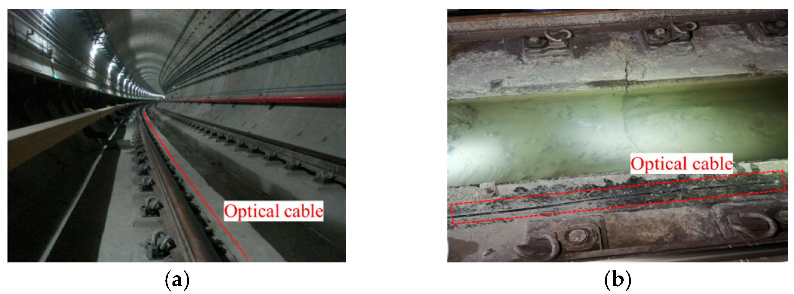
The investigated structure is a 39-km-long underground railway track in China; it operates entirely underground and has been in service for six years. The UWFBG sensing system was continuously installed on the surface of track beds parallel to the track, as depicted in Figure 2a. Figure 2b provides a zoom-in view of the optical cable, illustrating the adhesive bonding method used to secure the optical cable to the concrete track bed.
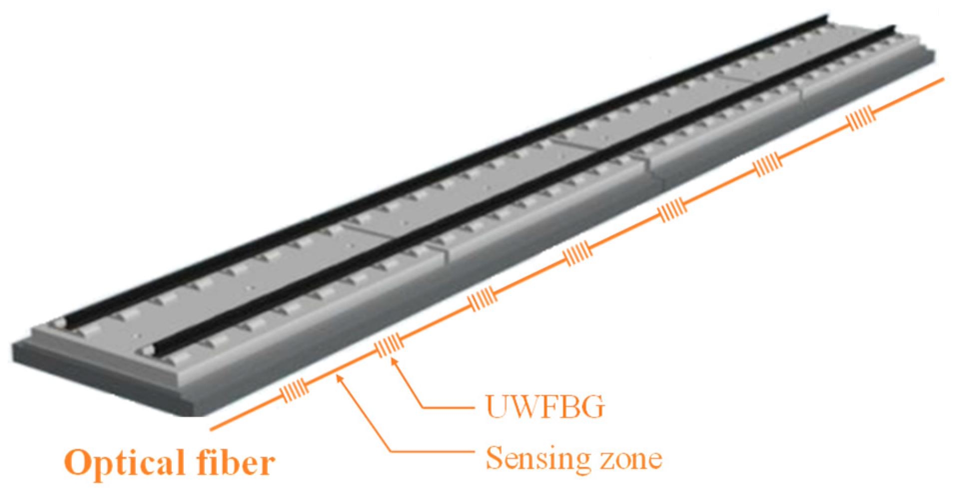
Figure 3 illustrates the optical cable, which employs UWFBGs. A distinguishing feature of UWFBGs is their extraordinarily low reflectivity, enabling the multiplexing of thousands of sensors on a single optical cable. The smallest sensing unit within the UWFBG system is referred to as the sensing zone, which comprises two adjacent UWFBGs and the optical fiber situated between them. UWFBG system operates by detecting the phase change of reflected light due to micro-vibrations between adjacent UWFBGs. Consequently, the vibration response measured by each sensing zone signifies the average dynamic strain endured by the optical fiber within that area. The UWFBG system achieves a strain measurement resolution of , with the distance between adjacent UWFBGs determining the size of the sensing zones, designed at 5 m. The system samples vibration responses at a frequency of 1000 Hz.
The investigated railway track structure comprises two types of track beds: the general integral track beds (GIT, as depicted in Figure 4a) and the steel spring floating slab track beds (SSFT, as shown in Figure 4b). The primary distinction lies in the fact that the GIT is in direct contact with the concrete base, while the SSFT is supported by steel spring isolators (highlighted in blue in Figure 4b) on the concrete base, forming a mass–spring–damper system. Consequently, compared to the GIT, the SSFT exhibits significantly enhanced vibration and noise reduction effects. Furthermore, the vibration responses collected by the UWFBG system installed on both types of track beds under train loads display markedly different patterns, as illustrated in Figure 5.
Figure 5 showcases the typical dynamic response collected from GIT and SSFT under train loads. The vibration response from the GIT exhibits a more consistent pattern compared to that of the SSFT, with response peaks coinciding with the load time of the train wheels. As depicted in Figure 5a, the vibration signal when a train comprising six carriages passes by is clearly discernible. Conversely, the vibration response duration of the SSFT is longer, approximately twice that of the GIT. This is attributed to the interference signals generated by the vibration of adjacent track beds.
3.2. Dataset Construction
The sampling frequency of the UWFBG system is 1000 Hz, while the maximum frequency component of the vibration responses typically does not exceed 100 Hz. Therefore, in accordance with the Shannon sampling theorem, the original monitoring data are initially filtered and subsequently down-sampled. This leads to a re-adjusted sampling frequency of 200 Hz, which contributes to a substantial reduction in data volume and significantly enhances the efficiency of subsequent data analysis.
The UWFBG system operated at a sampling frequency of 1000 Hz. However, the maximum frequency component of the vibration responses typically does not exceed 100 Hz. Therefore, in accordance with the Shannon sampling theorem, the original monitoring data were initially filtered and subsequently down-sampled. This leads to a re-adjusted sampling frequency of 200 Hz, which contributes to a substantial reduction in data volume and significantly enhances the efficiency of subsequent data analysis.
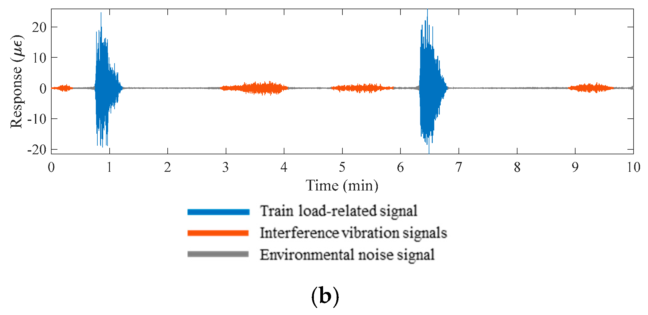
To extract samples from the long-term monitoring data, a sliding fixed-size window in the time domain is employed. Specifically, the window size is set to 10 min, approximately twice the interval time for train passing. This ensures each sample covers at least one train passing event and contains 120,000 data points. Figure 6 presents two typical samples extracted from the monitoring data of GIT and SSFT. The samples primarily comprise train-induced signals, environmental noise signals, and interference vibration signals. Generally, the train-induced signals display the largest amplitude and typically last between 10 and 20 s, determined by the type of track bed and the speed of the train. The environmental noise signals have the longest duration, with their amplitudes almost zero. The interference vibration signals fall between the previous two categories in terms of amplitude and could be attributed to ground vehicles, construction activities, or other factors. The amplitudes and durations of these interference vibration signals exhibit a higher degree of randomness.
The proposed method aims to extract passing-train signals, defined as the vibration responses of tracks subjected to immediate wheel loads. These passing-train signals form a portion of the train-induced signals, and different labeling principles should be applied to different types of track beds. Figure 7 offers an illustrative view and the spectrogram of train-induced signals of a GIT, as seen in Figure 6a. Given the significant stiffness of the GIT and its isolation from adjacent track beds, the train-induced signals mainly stem from the immediate wheel loads. This is substantiated by the spectrogram, which demonstrates that the main energy of passing-train signals is located around 5 Hz. Consequently, the train-induced signals align with the desired passing-train signals, as denoted by the blue box in Figure 7. A key characteristic of the passing-train signals of GIT is a quick increase in amplitude (labeled as the start point), followed by a rapid decrease after a certain duration (labeled as the endpoint), typically ranging from 10 to 20 s.
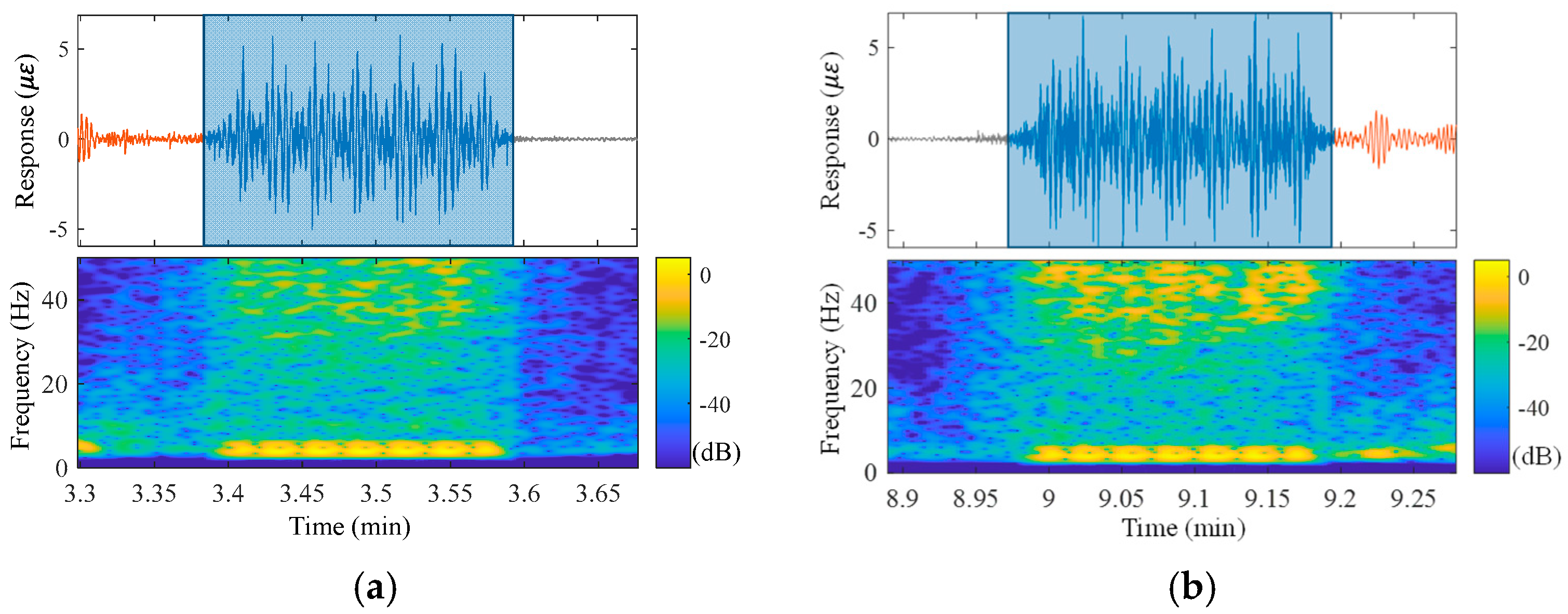
Distinct from GIT, the train-induced signals of the SSFT structure generally consist of passing-train signals within the middle segment, while the terminal portions are occupied by responses of different modes, mainly instigated by the vibrations of adjacent track beds. As depicted in Figure 8, the response arising from immediate wheel loads comprises frequency components predominantly lower than 10 Hz. To improve the quality of the monitoring dataset and the efficiency of subsequent structural condition assessment methods, it is crucial to eradicate the signals of abnormal modes at both ends of the train load-related signals, retaining only the passing-train signals. As such, the labeling principle for the SSFT signals should not be solely dependent on the time domain information but should integrate the spectrogram as well. As marked in the red boxes in the time-frequency domain of Figure 8, the start and endpoints of the passing-train signals are positioned at the shift points of the spectrogram to conserve a signal period with a recognizable low-frequency component.
The UWFBG sensing system installed on the investigated urban railway track contains over 15,000 sensing zones. Through random sampling, 1200 samples of 10-min length were selected and manually labeled, among which the number of samples collected from GIT and SSFT were the same, both being 600. To boost the efficiency of segmentation methods, all labeled samples are further down-sampled to 50 Hz. As a result, each sample consists of 30,000 data points.
3.3. Results of the Traditional Dual-Threshold Method
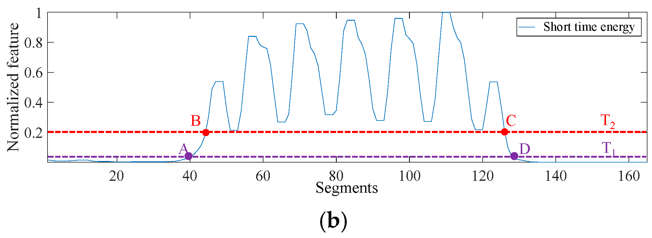
The traditional dual-threshold method, established for VAD, employs two thresholds of features, and (where ), for signal segment classification. Initially, the original data are subdivided into smaller segments using sliding windows; subsequently, each segment is assigned its respective feature value, as illustrated in Figure 9, where the data are transformed into a series of short-term energy feature values. As expected, the magnitude of short-term energy features escalates as the original data’s amplitude increase. The threshold aims to roughly categorize the target segments—any segment with a feature value surpassing is recognized as a target segment (as depicted between points B and C in Figure 9). The threshold , on the other hand, forms the boundary of these target segments. To fulfill this, a search springs from both ends of the target segments (determined by ) until the first intersection points with emerge (points A and D in Figure 9), thus marking the final target segments from point A to D. Consequently, all data within these segments are identified as the passing-train signals.
The dual-threshold strategy is usually merged with multiple features of the original data to ensure a more reliable segmentation. Furthermore, the intersections of the target signals arising from these features were regarded as the outcome. The classic dual-threshold method predominantly employs short-term energy (STE) and the short-term zero-crossing rate (ZCR) as its most common features.
Figure 7 and Figure 8 demonstrate the obvious differences between the train-induced signals and other signals in the time-frequency domain. Specifically, the main energy of the passing-train signals is focused on frequency components below 10 Hz. Consequently, this study introduces the STLFE to effectively discern the passing-train signals. This feature is incorporated alongside the STE into the dual-threshold strategy. The mathematical expressions for both STE and STLFE can be observed in Equations (6) and (7).
where denotes the short-time energy of the i-th segment; denotes the n-th data point of the signal within the i-th segment; is the number of data points per segment; denotes the short time low-frequency energy of the i-th segment, denotes the magnitude of the k-th frequency bin in the spectrum of ; is the index of the frequency point corresponding to the upper limit of frequency range researched (0–10 Hz in this paper) in the spectrum.
Appropriate post-processing is essential for enhancing the dual-threshold strategy, including the fusion of adjacent passing-train signals and the elimination of short-duration passing-train signals. The hyperparameters associated with the proposed dual-threshold approach are listed in Table 1. The merge distance is set to 1, indicating that passing-train signals detected within an interval of less than 1 s are merged. The minimum duration is set to 5, implying that passing-train signals identified to persist for less than 5 s are discarded.
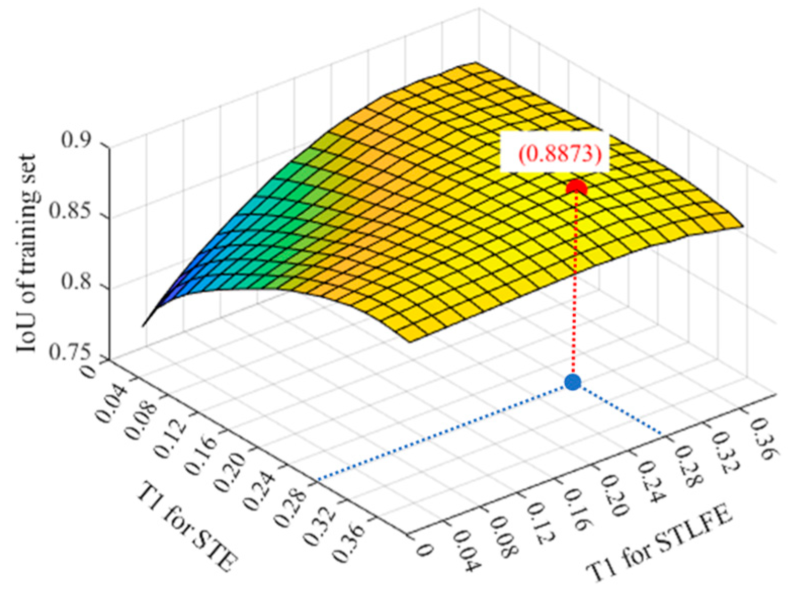
Moreover, the optimal T2 for the normalized STE and STLFE is determined to be 0.4 after several attempts, and the optimal T1 is searched within the range of 5% to 95% of T2, with a 5% interval. As shown in Figure 10, the mean IoU of the manually labeled dataset varies with T1 for both STE and STLFE. In the end, the optimal T1 for both the STE and STLFE is determined to be 0.28, with the highest mean IoU achieved at 0.887.
3.4. Results of the Proposed U-Net-1D Approach
The manually labeled dataset is composed of 1200 samples, 900 of which are assigned to the training dataset, 100 to the validation dataset, and the remaining 200 to the test dataset. These samples, randomly allocated, have their amplitudes normalized within the confines of [−1, 1]. The training parameters for the U-net-1D model are detailed in Table 2, employing a stepwise learning rate strategy. Under this approach, the learning rate is halved at every 50-epoch interval. The model is trained with a batch size of 64 across a total of 200 epochs.
The convolutional kernel size notably impacts the U-net-1D’s performance. To ascertain the ideal kernel size, U-net-1D models utilizing kernels of sizes 3, 5, 15, and 25 undergo training for comparative analysis. Figure 11 showcases the typical segmentation results derived from a sample taken from the SSFT. The observed trends indicate that smaller convolutional kernels engender a more refined segmentation granularity, thereby facilitating the identification of a greater number of candidate segments. Conversely, larger convolutional kernels promote smoother predictions.
To perform pointwise segmentation, a fixed decision boundary is employed. Data points boasting predicted probabilities surpassing this boundary are categorized as passing-train signals. To curtail the impact of misidentified signals, the post-processing method as well as its parameters used for U-net-1D are consistent with the dual-threshold method.
The performance of U-net-1D with varying kernel sizes across the training dataset, validation dataset, and test dataset is detailed in Table 3, where the decision boundary is set to 0.5. The last row of Table 3 shows the segmentation results of the dual-threshold method. The IoU and Precision for U-net-1D with smaller kernel sizes (3 and 5) surpass that of the models with larger kernel sizes (15 and 25) and the dual-threshold method. This implies that models carrying smaller kernel sizes exhibit superior segmentation efficacy. U-net-1D consistently posts Recalls exceeding those of the dual-threshold method, nearing a perfect 100%; this denotes U-net-1D’s enhanced ability to identify positive data points—passing-train signals. Furthermore, the Recalls of the U-net-1D are higher than the corresponding Precisions, which indicates that the U-net-1D is conservative and the identified segments generally cover the labeled regions, as shown in Figure 12.
To enhance the IoU, the decision boundary is elevated to 0.9, with the corresponding results presented in Table 4. Upon comparing with Table 3, it is evident that the U-net-1D models, with their varying kernel sizes, have achieved superior IoU for the testing dataset as the decision boundary increased. A kernel size of 5 yielded the highest IoU at 94.27%, which is a commendable outcome considering the inherent randomness involved in the manual labeling process. Given that IoU is a more comprehensive metric than Precision and Recall, a kernel size of 5 is deemed the optimal choice for this study.
Table 5 presents the comparative analysis of segmentation results for samples from GIT and SSFT, with the kernel size configured to 5 and the decision boundary set to 0.9. The results reveal that U-net-1D significantly outperforms in segmenting the monitoring data of GIT as compared to SSFT. This outcome aligns with intuitive expectations, given the complexity of interference signals in SSFT’s monitoring data.
The visualization of segmentation results for consecutive sensing zones is shown in Figure 13. Specifically, Figure 13a presents a heatmap composed of amplitude data from consecutive sensing zones numbered from 1 to 220. The horizontal axis indicates the zone number, while the vertical axis represents time. Thus, each column of data corresponds to a 10-min sample of monitoring data from a specific sensing zone. Sensing zones 1–53 consist of GIT beds, whereas sensing zones 54–220 consist of SSFT beds. Given the directionality of train movement from smaller-numbered sensing zones to larger ones in the track monitored, corresponding train-induced signals appear in the heatmap as a negatively sloped highlighted area. Conversely, positively sloped highlighted zones in the heatmap are attributable to interference vibration signals produced by trains operating in the opposite direction on adjacent tracks. Figure 13a also exhibits randomly dispersed environmental noise signals, evident in the randomly positioned vertical highlights throughout the figure. Figure 13b presents the binary segmentation results of data from Figure 13a using the proposed U-net-1D, where the white zones signify recognized passing train signals. It is evident that the U-net method successfully avoids disturbances from environmental noise and interference vibration signals, thereby adaptively recognizing passing train signals.
4. Conclusions
This study introduced an adaptive monitoring system that can automatically identify and retain the passing-train signals during the data preprocessing process while eliminating non-essential signals like environmental noise and interference vibration signals. A U-net model with one-dimensional convolution layers (U-net-1D) is proposed for efficient pointwise segmentation of vibration monitoring data. For comparison, a dual-threshold method integrating the short-term energy (STE) and short-term low-frequency energy (STLFE) features is also presented. The main conclusions are as follows:
- (1)
- Inspired by image semantic segmentation, the proposed U-net-1D model is capable of identifying the train-induced vibration signals collected by the UWFBG sensing system in pointwise segmentation with high accuracy. When the convolutional kernel size is 5, and the decision boundary is 0.9, the U-net-1D model achieved a remarkable mean Intersection over Union (IoU) of 94.27% on the test dataset, validating its profound accuracy.
- (2)
- In comparison with the traditional dual-threshold method, the U-net-1D model consistently yields superior metrics, including IoU, Precision, and Recall, across all stages including training, validation, and testing. This clearly demonstrates its effectiveness and accuracy.
- (3)
- Considering that passing-train signals constitute less than 7% of total monitoring time, leveraging the U-net-1D model for the data preprocessing stage holds great promise for reducing data storage costs, thereby highlighting the considerable practical potential of the proposed method.
Author Contributions
Conceptualization, Q.L.; data curation, S.Z.; formal analysis, J.C.; funding acquisition, J.C., C.L. and S.W.; investigation, J.C.; methodology, S.W.; project administration, Q.L., S.Z. and C.L.; resources, Q.L., S.Z. and C.L.; software, J.C.; supervision, Q.L.; validation, J.C., S.Z. and C.L.; visualization, J.C.; writing—original draft, J.C.; writing—review and editing, S.W. All authors have read and agreed to the published version of the manuscript.
Funding
This research was funded by the Key Research Project of China Railway Siyuan Survey and Design Group Co., Ltd., grant number KY2023001S, the China Postdoctoral Science Foundation, grant number 2023M744101, the Funding for the Postdoctoral Innovative Practice Position in Hubei Province for the 2022–2023 year, the National Natural Science Foundation of China, grant number 52208311, Major scientific and technological R & D projects of China Railway Construction Co., Ltd., grant number 2021-A03, and Young Elite Scientists Sponsorship Program by CAST, grant number 2021QNRC001.
Data Availability Statement
The data presented in this study are available on request from the corresponding author. The data are not publicly available due to privacy.
Conflicts of Interest
Authors Jiahui Chen, Qiuyi Li, Shijie Zhang and Chao Lin were employed by the company China Railway Siyuan Survey and Design Group Co., Ltd. The remaining author declares that the research was conducted in the absence of any commercial or financial relationships that could be construed as a potential conflict of interest.
References
- Li, Q.; Huang, Y.; Chen, J.; Liu, X.; Meng, X.; Lin, C. Feature Selection and Damage Identification for Urban Railway Track Using Bayesian Globally Sparse Principal Component Analysis. Sustainability 2023, 15, 5391. [Google Scholar] [CrossRef]
- Malekloo, A.; Ozer, E.; AlHamaydeh, M.; Girolami, M. Machine learning and structural health monitoring overview with emerging technology and high-dimensional data source highlights. Struct. Health Monit. 2022, 21, 1906–1955. [Google Scholar] [CrossRef]
- Bao, Y.; Chen, Z.; Wei, S.; Xu, Y.; Tang, Z.; Li, H. The state of the art of data science and engineering in structural health monitoring. Engineering 2019, 5, 234–242. [Google Scholar] [CrossRef]
- Gordan, M.; Sabbagh-Yazdi, S.R.; Ismail, Z.; Ghaedi, K.; Carroll, P.; McCrum, D.; Samali, B. State-of-the-art review on advancements of data mining in structural health monitoring. Measurement 2022, 193, 110939. [Google Scholar] [CrossRef]
- Liu, F.; Xu, B.; Wang, H.; Jiang, J.; Li, S.; Li, Z. Online long-distance monitoring of subway vibration reduction effect using ultra-weak fiber Bragg grating arrays. Measurement 2023, 217, 113057. [Google Scholar] [CrossRef]
- Nan, Q.; Li, S.; Yao, Y.; Li, Z.; Wang, H.; Wang, L.; Sun, L. A novel monitoring approach for train tracking and incursion detection in underground structures based on ultra-weak FBG sensing array. Sensors 2019, 19, 2666. [Google Scholar] [CrossRef] [PubMed]
- Jalil, M.; Butt, F.A.; Malik, A. Short-time energy, magnitude, zero crossing rate and autocorrelation measurement for discriminating voiced and unvoiced segments of speech signals. In Proceedings of the International Conference on Technological Advances in Electrical, Electronics and Computer Engineering (TAEECE), Konya, Turkey, 9–11 May2013; pp. 208–212. [Google Scholar]
- Zhang, A.; Yang, B.; Huang, L. Feature Extraction of EEG Signals Using Power Spectral Entropy. In Proceedings of the 2008 International Conference on BioMedical Engineering and Informatics, Sanya, China, 28–30 May 2008; Volume 2, pp. 435–439. [Google Scholar]
- Davis, A.; Nordholm, S.; Togneri, R. Statistical Voice Activity Detection Using Low-Variance Spectrum Estimation and an Adaptive Threshold. IEEE Trans. Audio Speech Lang. Process. 2006, 14, 412–424. [Google Scholar] [CrossRef]
- Muda, L.; Begam, M.; Elamvazuthi, I. Voice Recognition Algorithms Using Mel Frequency Cepstral Coefficient (MFCC) and Dynamic Time Warping (DTW) Techniques. arXiv 2010, arXiv:1003.4083. [Google Scholar]
- Zhang, T.; Shao, Y.; Wu, Y.; Geng, Y.; Fan, L. An Overview of Speech Endpoint Detection Algorithms. Appl. Acoust. 2020, 160, 107133. [Google Scholar] [CrossRef]
- Yiming, S.; Rui, W. Voice Activity Detection Based on the Improved Dual-Threshold Method. In Proceedings of the 2015 International Conference on Intelligent Transportation, Big Data and Smart City, Halong Bay, Vietnam, 19–20 December 2015; pp. 996–999. [Google Scholar]
- Jiang, N.; Liu, T. An Improved Speech Segmentation and Clustering Algorithm Based on SOM and k-means. Math. Probl. Eng. 2020, 2020, 3608286. [Google Scholar] [CrossRef]
- Roy, T.; Marwala, T.; Chakraverty, S. Precise Detection of Speech Endpoints Dynamically: A Wavelet Convolution Based Approach. Commun. Nonlinear Sci. Numer. Simulat. 2019, 67, 162–175. [Google Scholar] [CrossRef]
- Ma, Y.; Nishihara, A. Efficient Voice Activity Detection Algorithm Using Long-Term Spectral Flatness Measure. Eurasip. J. Audio Speech Music. Process. 2013, 2013, 87. [Google Scholar] [CrossRef]
- Bao, J.; Mo, J.; Xu, L.; Liu, Y.; Lv, X. VMD-Based Vibrating Fiber System Intrusion Signal Recognition. Optik 2020, 205, 163753. [Google Scholar] [CrossRef]
- Liu, H.; Ma, J.; Yan, W.; Liu, W.; Zhang, X.; Li, C. Traffic Flow Detection Using Distributed Fiber Optic Acoustic Sensing. IEEE Access 2018, 6, 68968–68980. [Google Scholar] [CrossRef]
- Gaugel, S.; Reichert, M. PrecTime: A Deep Learning Architecture for Precise Time Series Segmentation in Industrial Manufacturing Operations. Eng. Appl. Artif. Intell. 2023, 122, 106078. [Google Scholar] [CrossRef]
- Perslev, M.; Jensen, M.; Darkner, S.; Jennum, P.J.; Igel, C. U-Time: A Fully Convolutional Network for Time Series Segmentation Applied to Sleep Staging. In Advances in Neural Information Processing Systems; MIT Press: Cambridge, MA, USA, 2019; Volume 32. [Google Scholar]
- Londhe, A.N.; Atulkar, M. Semantic Segmentation of ECG Waves Using Hybrid Channel-Mix Convolutional and Bidirectional LSTM. Biomed. Signal Process. Control. 2021, 63, 102162. [Google Scholar] [CrossRef]
- Shang, Z.; Xia, Y.; Chen, L.; Sun, L. Damping Ratio Identification Using Attenuation Responses Extracted by Time Series Semantic Segmentation. Mech. Syst. Signal Process. 2022, 180, 109287. [Google Scholar] [CrossRef]
- Ronneberger, O.; Fischer, P.; Brox, T. U-Net: Convolutional Networks for Biomedical Image Segmentation. In Proceedings of the Medical Image Computing and Computer-Assisted Intervention—MICCAI 2015: 18th International Conference, Munich, Germany, 5–9 October 2015. [Google Scholar]
- Yu, C.; Wang, J.; Peng, C.; Gao, C.; Yu, G.; Sang, N. Bisenet: Bilateral segmentation network for real-time semantic segmentation. In Proceedings of the European Conference on Computer Vision (ECCV), Glasgow, UK, 8–14 September 2018; pp. 325–341. [Google Scholar]
- Guo, Y.; Liu, Y.; Georgiou, T.; Lew, M.S. A Review of Semantic Segmentation Using Deep Neural Networks. Int. J. Multimed. Inf. Retr. 2018, 7, 87–93. [Google Scholar] [CrossRef]
- Zhao, J.; Hu, F.; Qiao, W.; Zhai, W.; Xu, Y.; Bao, Y.; Li, H. A Modified U-Net for Crack Segmentation by Self-Attention-Self-Adaption Neuron and Random Elastic Deformation. Smart Struct. Syst. 2022, 29, 1–16. [Google Scholar]
- Huang, H.; Lin, L.; Tong, R.; Hu, H.; Zhang, Q.; Iwamoto, Y.; Han, X.; Chen, Y.W.; Wu, J. Unet 3+: A Full-Scale Connected Unet for Medical Image Segmentation. In Proceedings of the ICASSP 2020–2020 IEEE International Conference on Acoustics, Speech and Signal Processing (ICASSP), Barcelona, Spain, 4–8 May 2020; pp. 1055–1059. [Google Scholar]
- Cao, H.; Wang, Y.; Chen, J.; Jiang, D.; Zhang, X.; Tian, Q.; Wang, M. Swin-Unet: Unet-Like Pure Transformer for Medical Image Segmentation. In Proceedings of the European Conference on Computer Vision; Springer Nature: Cham, Switzerland, 2022; pp. 205–218. [Google Scholar]
- Wang, C.; MacGillivray, T.; Macnaught, G.; Yang, G.; Newby, D. A Two-Stage 3D Unet Framework for Multi-Class Segmentation on Full Resolution Image. arXiv 2018, arXiv:1804.04341. [Google Scholar]
- He, X.; Zhou, Y.; Zhao, J.; Zhang, D.; Yao, R.; Xue, Y. Swin Transformer Embedding UNet for Remote Sensing Image Semantic Segmentation. IEEE Trans. Geosci. Remote Sens. 2022, 60, 4408715. [Google Scholar] [CrossRef]
- Jadon, S. A Survey of Loss Functions for Semantic Segmentation. In Proceedings of the 2020 IEEE Conference on Computational Intelligence in Bioinformatics and Computational Biology (CIBCB), Virtual, 27–29 October 2020; pp. 1–7. [Google Scholar]
Figure 1.
Semantic segmentation of monitoring data using U-net-1D.

Figure 2.
Optical cable installed on the surface of track beds: (a) a global perspective and (b) a zoom-in view.
Figure 2.
Optical cable installed on the surface of track beds: (a) a global perspective and (b) a zoom-in view.

Figure 3.
Schematic diagram of the optical cable.

Figure 4.
Cross-sections of two track beds: (a) GIT and (b) SSFT.

Figure 5.
Typical data patterns collected from (a) GIT and (b) SSFT.

Figure 6.
Typical dynamic responses collected from (a) GIT and (b) SSFT.


Figure 7.
The train-induced signals of GIT in Figure 6a: (a) the first passing and (b) the second passing. The blue boxes represent the duration of passing-train signals.
Figure 7.
The train-induced signals of GIT in Figure 6a: (a) the first passing and (b) the second passing. The blue boxes represent the duration of passing-train signals.

Figure 8.
The train-induced signals of SSFT in Figure 6b: (a) the first passing and (b) the second passing. The red boxes represent the duration of passing-train signals.
Figure 8.
The train-induced signals of SSFT in Figure 6b: (a) the first passing and (b) the second passing. The red boxes represent the duration of passing-train signals.

Figure 9.
An example of the traditional dual-threshold method: (a) the original data and (b) short-term energy feature.
Figure 9.
An example of the traditional dual-threshold method: (a) the original data and (b) short-term energy feature.


Figure 10.
Mean IoU varies with T1 for both STE and STLFE.

Figure 11.
Typical segmentation results using U-net-1D with different kernel sizes.

Figure 12.
Typical segmentation results of U-net-1D with Recall higher than Precision.

Figure 13.
Visualization of segmentation results for consecutive sensing zones: (a) amplitude heatmap and (b) binary segmentation results.
Figure 13.
Visualization of segmentation results for consecutive sensing zones: (a) amplitude heatmap and (b) binary segmentation results.


Table 1.
Hyperparameters of the dual-threshold method.
| Hyperparameter | Window Size | Overlap (%) | Merge Distance (s) | Minimum Duration (s) | T1 | T2 |
|---|---|---|---|---|---|---|
| Value | 128 | 90 | 1 | 5 | 0.28 | 0.4 |
Table 2.
Training parameters of U-net-1D.
| Hyperparameter | Initial Learning Rate | Drop Factor | Drop Period (Epoch) | Batch Size | Epoch |
|---|---|---|---|---|---|
| Value | 0.001 | 0.5 | 50 | 64 | 200 |
Table 3.
Results of U-net-1D with different kernel sizes (decision boundary is 0.5).
| Kernel Size | IoU (%) | Precision (%) | Recall (%) | ||||||
|---|---|---|---|---|---|---|---|---|---|
| Tra. | Val. | Te. | Tra. | Val. | Te. | Tra. | Val. | Te. | |
| 3 | 94.32 | 91.03 | 93.61 | 94.37 | 91.17 | 93.84 | 99.93 | 99.85 | 99.76 |
| 5 | 94.01 | 91.00 | 93.62 | 94.06 | 91.07 | 93.77 | 99.94 | 99.92 | 99.84 |
| 15 | 92.00 | 89.47 | 92.05 | 92.03 | 89.47 | 92.11 | 99.94 | 99.99 | 99.93 |
| 25 | 89.40 | 85.90 | 90.00 | 89.48 | 85.92 | 90.01 | 99.88 | 99.98 | 99.99 |
| Dual-threshold | 88.59 | 89.98 | 89.16 | 92.47 | 91.03 | 92.25 | 95.57 | 98.85 | 96.64 |
Note: Tra., Val., and Te. represent the training, validation, and test datasets, respectively. The optimal results are highlighted with an underline (same as below).
Table 4.
Results of U-net-1D with different kernel sizes (decision boundary is 0.9).
| Kernel Size | IoU (%) | Precision (%) | Recall (%) | ||||||
|---|---|---|---|---|---|---|---|---|---|
| Tra. | Val. | Te. | Tra. | Val. | Te. | Tra. | Val. | Te. | |
| 3 | 95.09 | 91.92 | 94.11 | 95.14 | 92.15 | 94.44 | 99.92 | 99.76 | 99.66 |
| 5 | 95.07 | 92.04 | 94.27 | 95.12 | 92.21 | 94.50 | 99.93 | 99.81 | 99.76 |
| 15 | 93.62 | 91.18 | 93.43 | 93.68 | 91.18 | 93.53 | 99.92 | 99.99 | 99.88 |
| 25 | 92.24 | 89.61 | 92.77 | 92.36 | 89.64 | 92.83 | 99.85 | 99.97 | 99.94 |
| Dual-threshold | 88.59 | 89.98 | 89.16 | 92.47 | 91.03 | 92.25 | 95.57 | 98.85 | 96.64 |
Table 5.
Comparisons of the results for GIT and SSFT.
| Track Type | IoU (%) | Precision (%) | Recall (%) | ||||||
|---|---|---|---|---|---|---|---|---|---|
| Tra. | Val. | Te. | Tra. | Val. | Te. | Tra. | Val. | Te. | |
| GIT | 96.33 | 93.71 | 96.53 | 96.35 | 93.82 | 96.78 | 99.98 | 99.88 | 99.74 |
| SSFT | 93.82 | 90.36 | 92.02 | 93.89 | 90.60 | 92.22 | 99.89 | 99.73 | 99.78 |
Disclaimer/Publisher’s Note: The statements, opinions and data contained in all publications are solely those of the individual author(s) and contributor(s) and not of MDPI and/or the editor(s). MDPI and/or the editor(s) disclaim responsibility for any injury to people or property resulting from any ideas, methods, instructions or products referred to in the content. |
© 2024 by the authors. Licensee MDPI, Basel, Switzerland. This article is an open access article distributed under the terms and conditions of the Creative Commons Attribution (CC BY) license (https://creativecommons.org/licenses/by/4.0/).
Share and Cite
MDPI and ACS Style
Chen, J.; Li, Q.; Zhang, S.; Lin, C.; Wei, S. Adaptive Vibration Monitoring of Railway Track Structures Using the UWFBG by the Identification of Train-Load Patterns. Buildings 2024, 14, 1239. https://doi.org/10.3390/buildings14051239
AMA Style
Chen J, Li Q, Zhang S, Lin C, Wei S. Adaptive Vibration Monitoring of Railway Track Structures Using the UWFBG by the Identification of Train-Load Patterns. Buildings. 2024; 14(5):1239. https://doi.org/10.3390/buildings14051239
Chicago/Turabian StyleChen, Jiahui, Qiuyi Li, Shijie Zhang, Chao Lin, and Shiyin Wei. 2024. "Adaptive Vibration Monitoring of Railway Track Structures Using the UWFBG by the Identification of Train-Load Patterns" Buildings 14, no. 5: 1239. https://doi.org/10.3390/buildings14051239
Note that from the first issue of 2016, this journal uses article numbers instead of page numbers. See further details here.