
New Method for Solving the Inverse Thermal Conduction Problem (θ-Scheme Combined with CG Method under Strong Wolfe Line Search)
 , and
, and
Abstract
:1. Introduction
2. The Mathematical Procedure
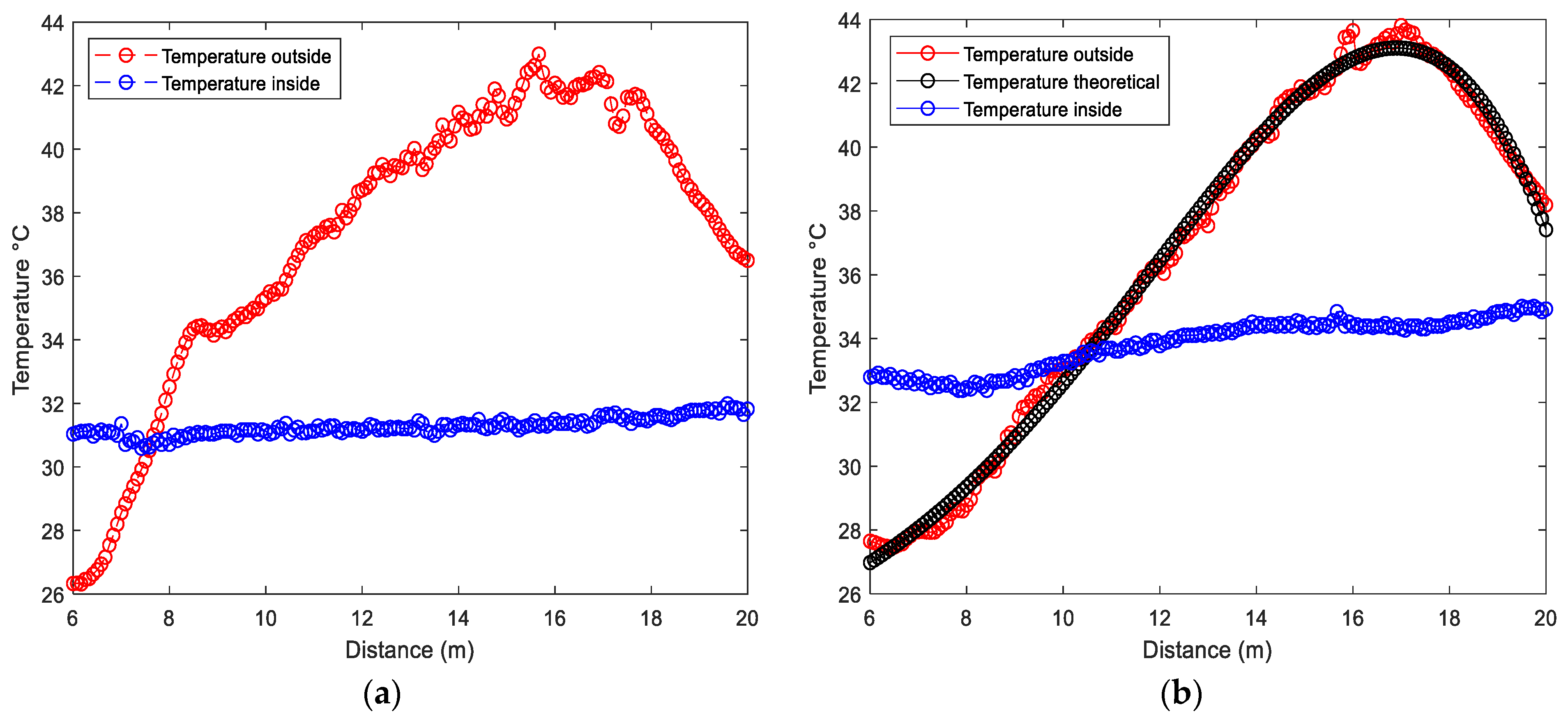
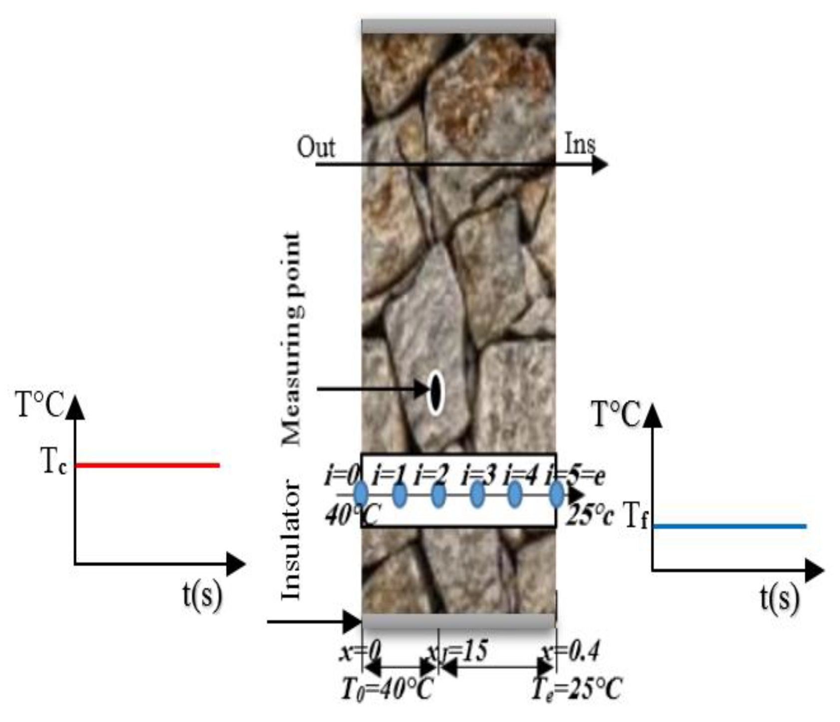
2.1. Validation of the Procedure
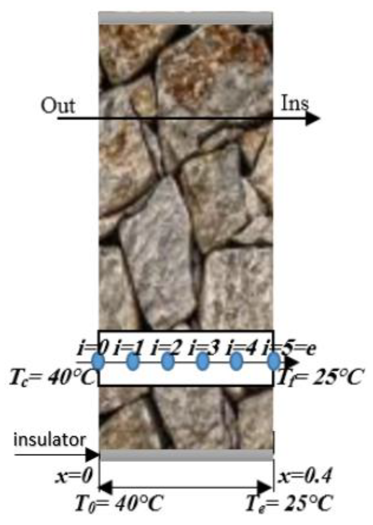
2.2. Direct Procedure
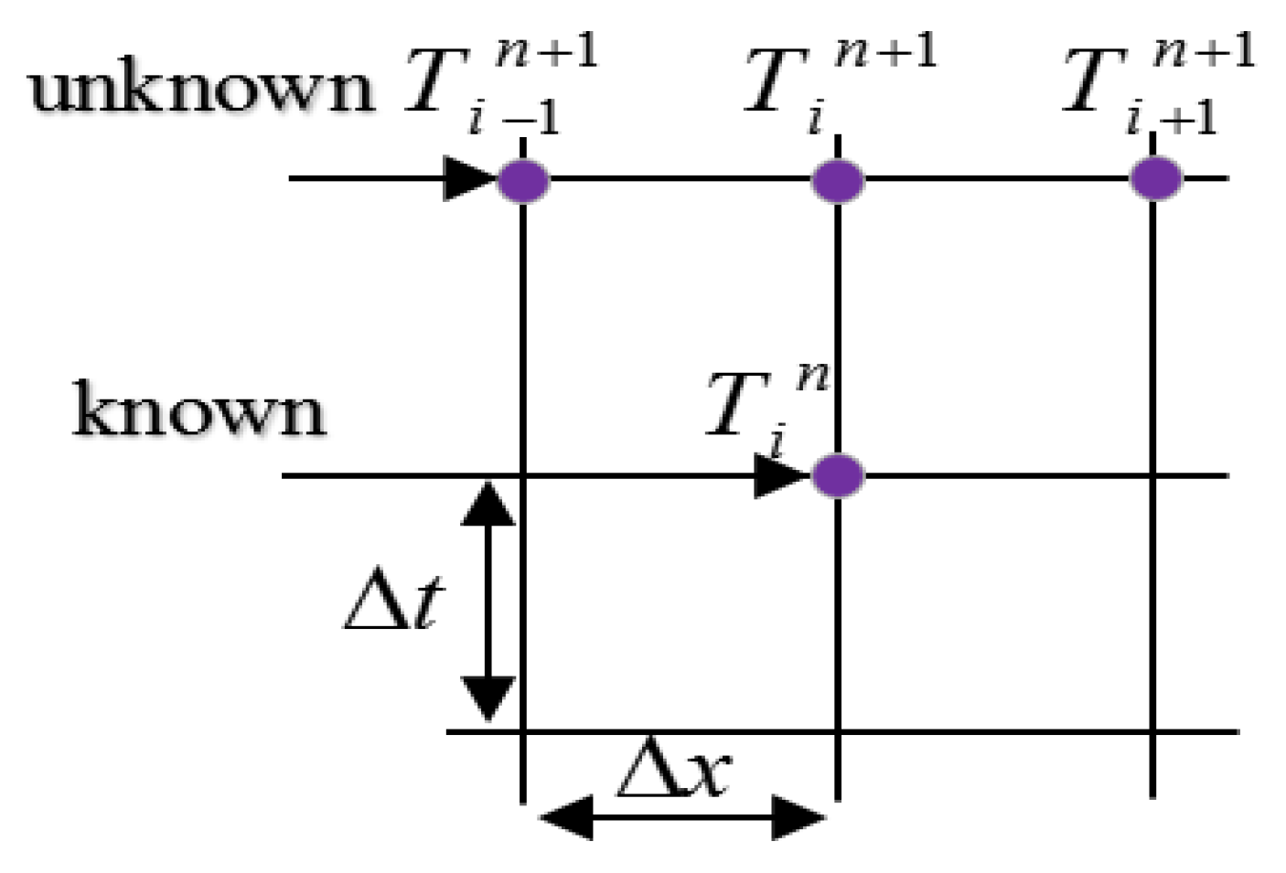
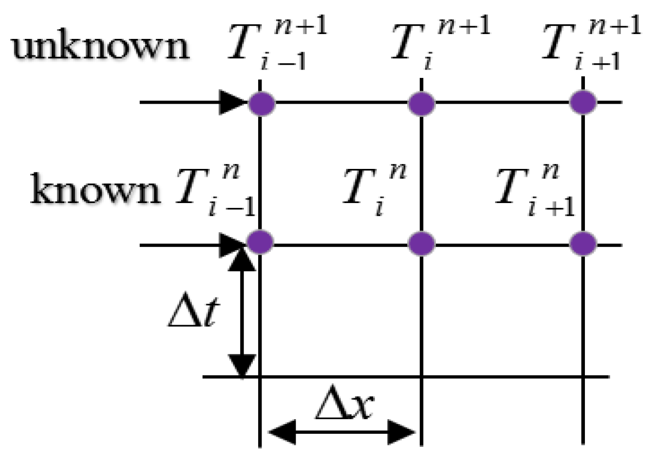
2.3. Explicit Form
2.4. Implicit Form
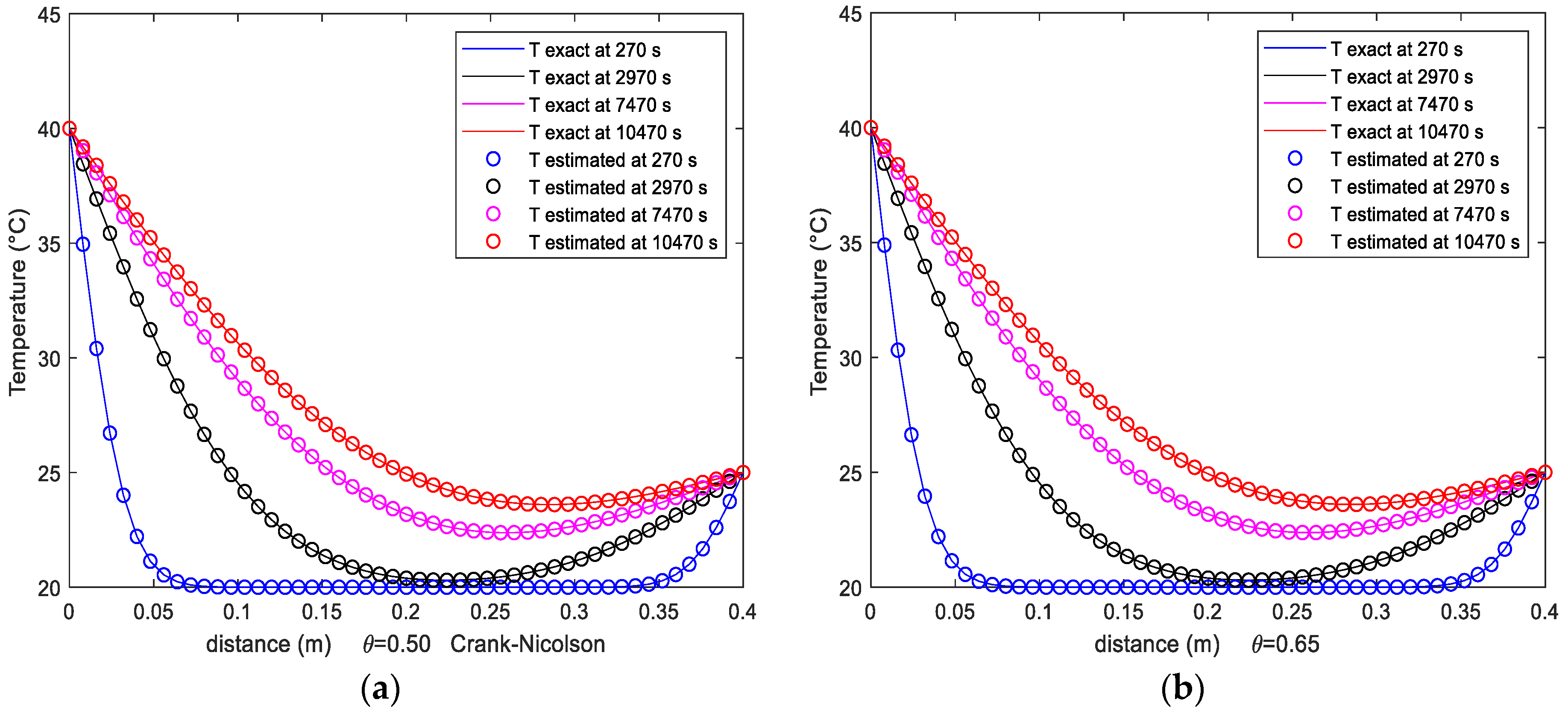
2.5. Crank–Nicolson Form
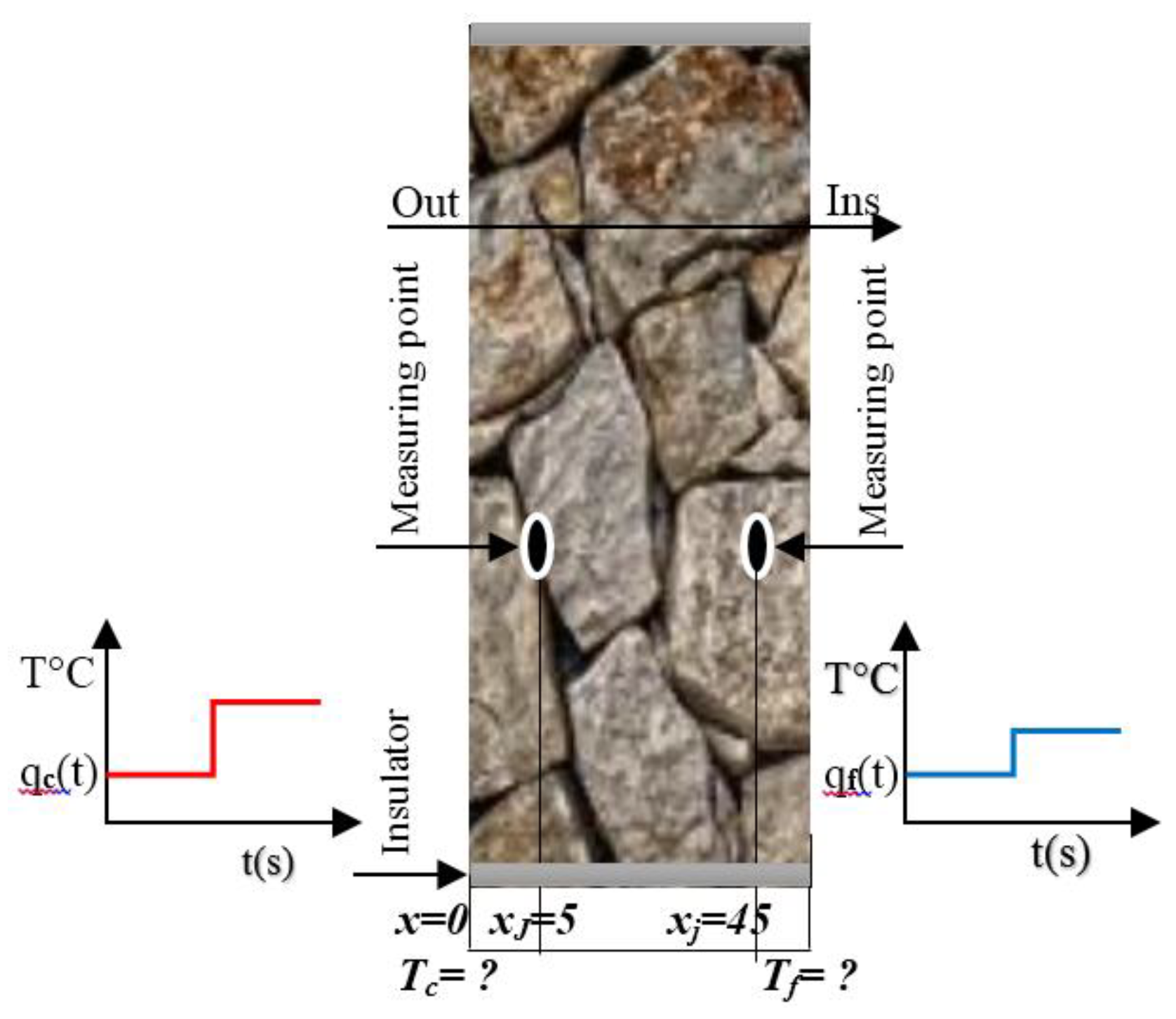
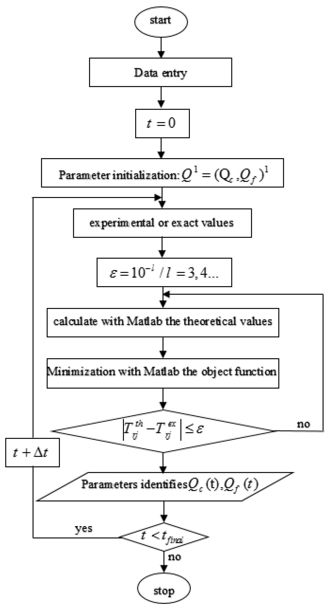
2.6. Inverse Procedure of θ-Scheme
- Approach 1.
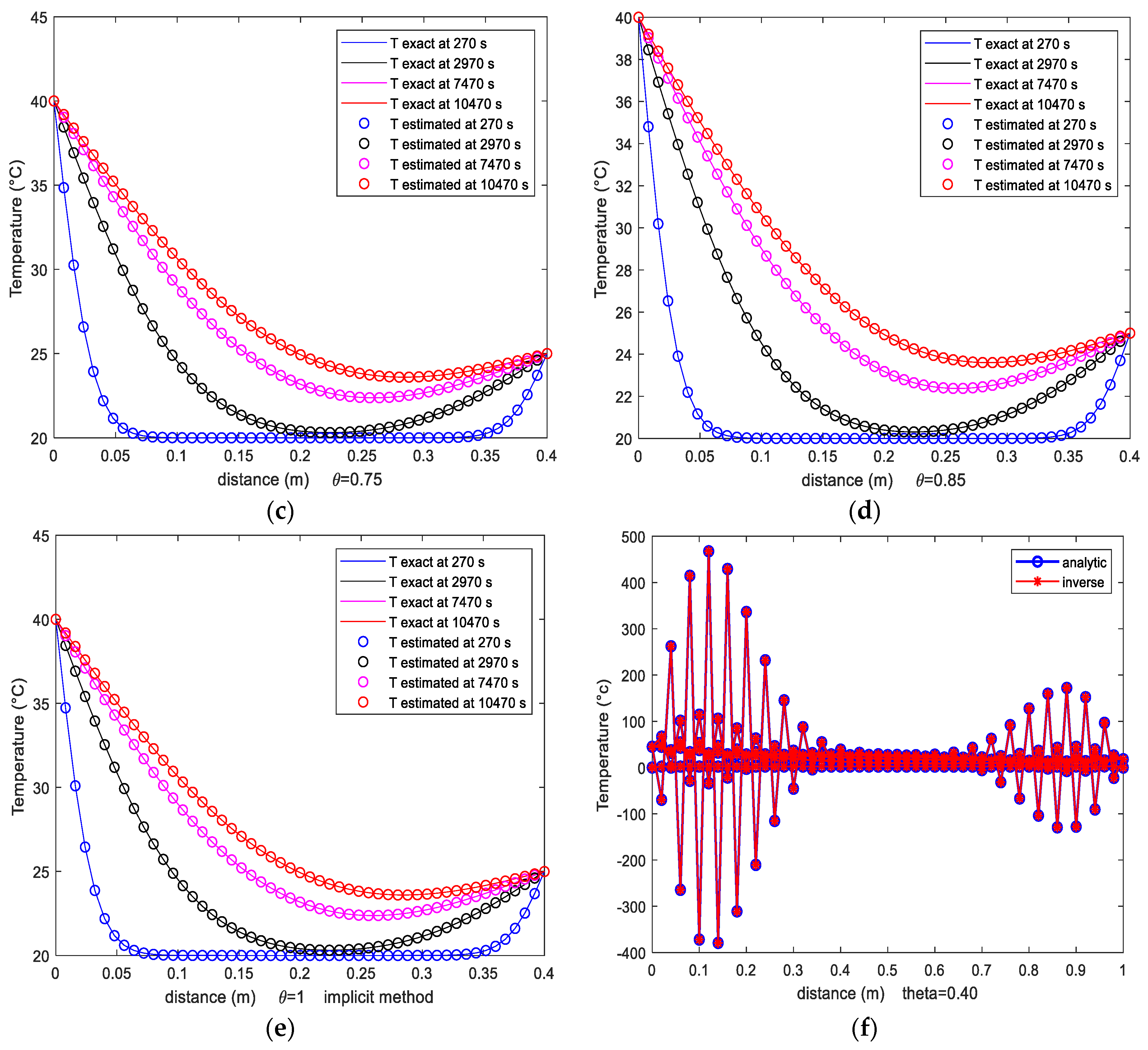
- For θ = 0, the θ-scheme (8) gives the explicit scheme.
- For θ = 1, the θ-scheme (8) leads to the implicit scheme.
- If θ = 0.5, the θ-scheme (14) gives the Crank–Nicolson scheme.
- Approach 2.
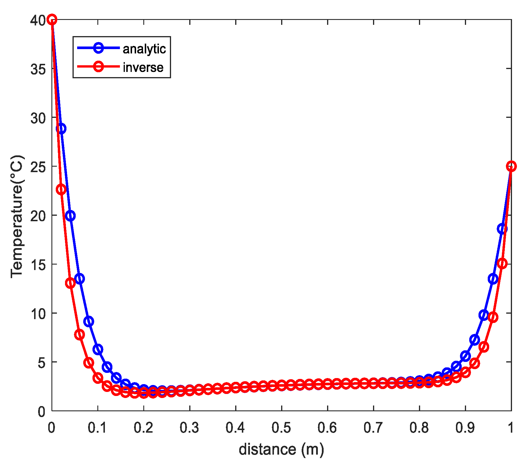
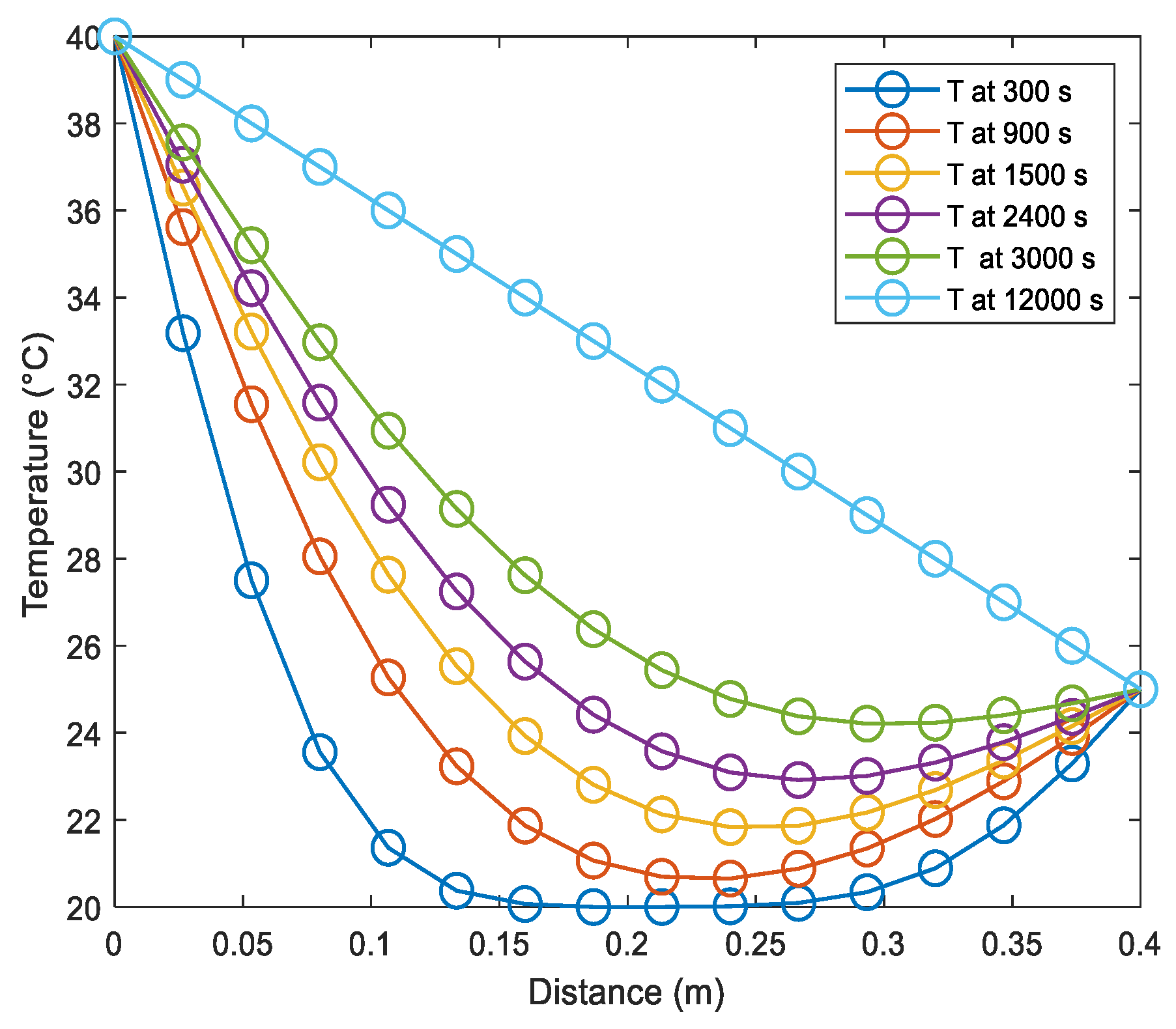
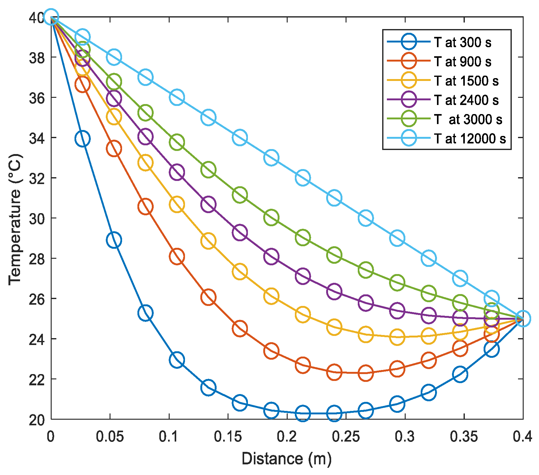
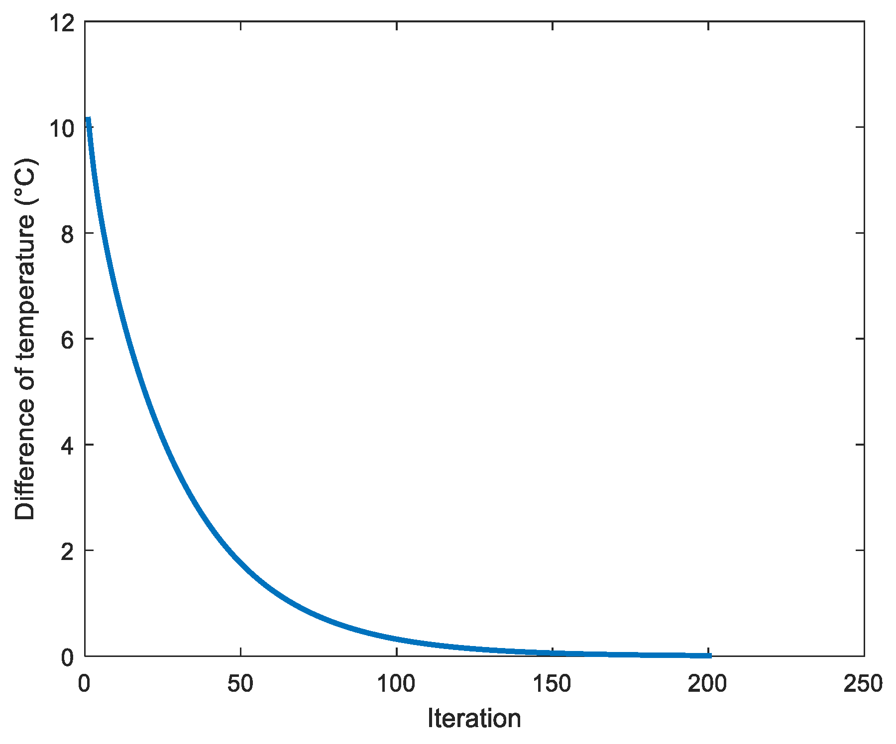
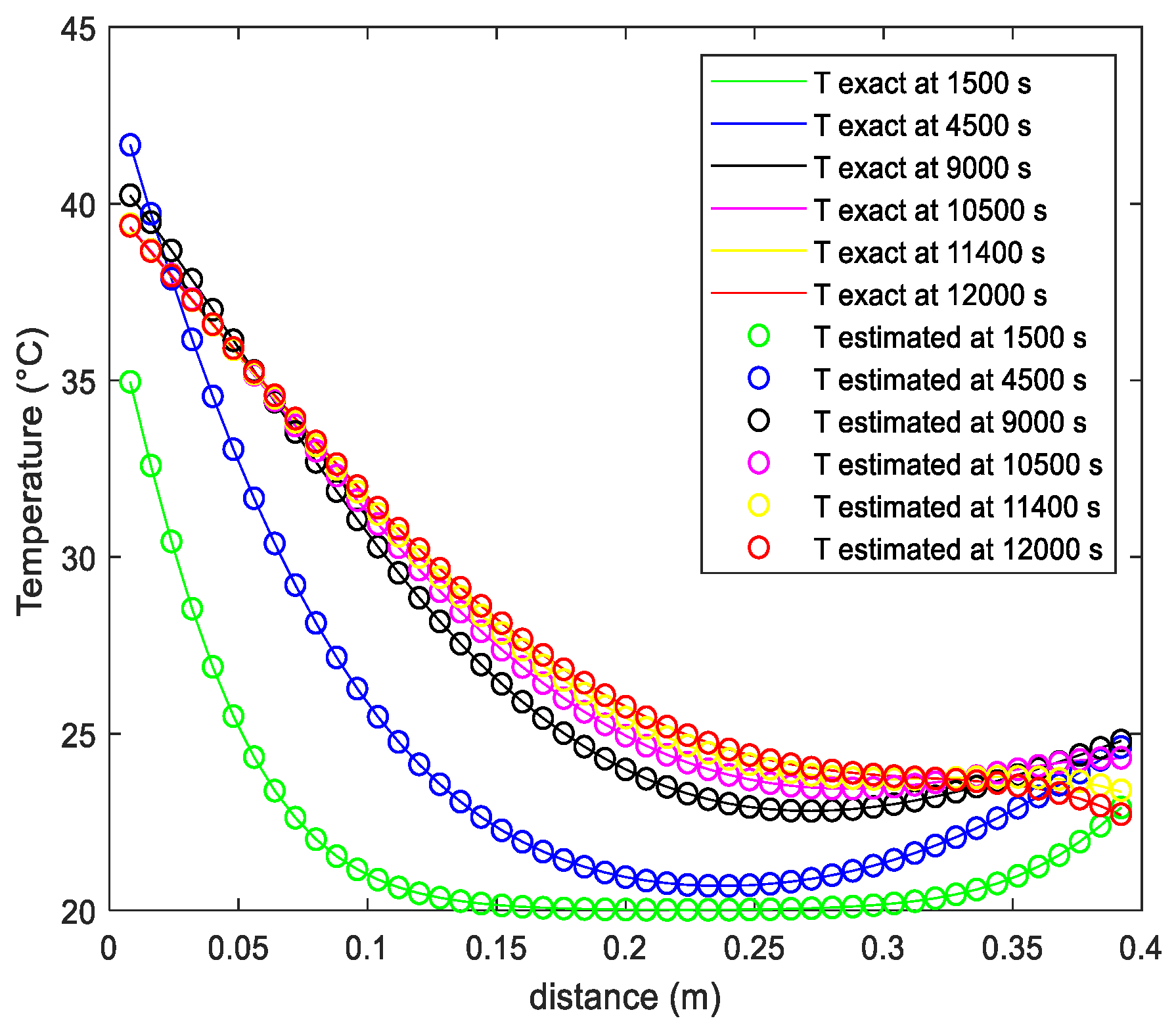
Numerical Results
- Example:
3. Conclusions
Author Contributions
Funding
Conflicts of Interest
Nomenclature
| θ: | real number |
| T: | temperature (°C) |
| t: | temps (s) |
| x: | distance (m) |
| ∆t: | time step |
| ∆x: | location step |
| e or L: | wall thickness (m) |
| n: | time index |
| k: | thermal conductivity (w/(m*k)) |
| ρ: | volumic mass (kg/m3) |
| Cp: | specific heat (J/(kg*K)) |
| α: | thermal diffusivity (m2/s) |
| : | hot side temperature (°C) |
| : | cold side temperature (°C) |
| CG: | gradient conjugate |
References
- Belgherras, S.; Bekkouche, S.M.A.; Benamrane, N. Prospective analysis of the energy efficiency in a farm studio under Saharan weather conditions. Energy Build. 2017, 145, 342–353. [Google Scholar] [CrossRef]
- Lalmi, D.; Benseddik, A.; Bensaha, H.; Bouzaher, M.T.; Arrif, T.; Guermoui, M.; Rabehi, A. Evaluation and estimation of the inside greenhouse temperature, numerical study with thermal and optical aspect. Int. J. Ambient. Energy 2019, 42, 1269–1280. [Google Scholar] [CrossRef]
- Bekkouche, S.; Benouaz, T.; Hamdani, M.; Cherier, M.; Yaiche, M.; Benamrane, N. Judicious choice of the building compactness to improve thermo-aeraulic comfort in hot climate. J. Build. Eng. 2015, 1, 42–52. [Google Scholar] [CrossRef]
- Bekkouche, S.; Benouaz, T.; Cheknane, A. A modelling approach of thermal insulation applied to a Saharan building. Therm. Sci. 2009, 13, 233–244. [Google Scholar] [CrossRef]
- Carbonari, A.; Naticchia, B.; D’Orazio, M. Innovative Evaporative cooling walls, Eco-Efficient Materials for Mitigating Building Cooling Needs. In Design, Properties and Applications; Woodhead: Cambridge, UK, 2015; pp. 215–240. Available online: http://www.sciencedirect.com/science/book/9781782423805 (accessed on 13 December 2022).
- Stojanovi, B.V.; Janevski, J.N.; Mitkovi, P.B.; Stojanovi, M.B.; Ignjatovi, M.G. Thermally activated building systems in context of increasing building energy efficiency. Therm. Sci. 2014, 18, 1011–1018. [Google Scholar] [CrossRef]
- Mohamed, Z.; Djafer, D.; Chouireb, F. New Approach to Establish a Clear Sky Global Solar Irradiance Model. Int. J. Renew. Energy Res. 2017, 7, 1454–1462. [Google Scholar]
- Rabehi, A.; Guermoui, M.; Lalmi, D. Hybrid models for global solar radiation prediction: A case study. Int. J. Ambient. Energy 2018, 41, 31–40. [Google Scholar] [CrossRef]
- Khelifi, R.; Guermoui, M.; Rabehi, A.; Lalmi, D. Multi-step-ahead forecasting of daily solar radiation components in the Saharan climate. Int. J. Ambient. Energy 2018, 41, 707–715. [Google Scholar] [CrossRef]
- Fang, Z.; Li, N.; Li, B.; Luo, G.; Huang, Y. The effect of building envelope insulation on cooling energy consumption in summer. Energy Build. 2014, 77, 197–205. [Google Scholar] [CrossRef]
- Choi, I.Y.; Cho, S.H.; Kim, J.T. Energy consumption characteristics of high-rise apartment buildings according to building shape and mixed-use development. Energy Build. 2012, 46, 123–131. [Google Scholar] [CrossRef]
- Castellani, B.; Morini, E.; Filipponi, M.; Nicolini, A.; Palombo, M.; Cotana, F.; Rossi, F. Clathrate Hydrates for Thermal Energy Storage in Buildings: Overview of Proper Hydrate-Forming Compounds. Sustainability 2014, 6, 6815–6829. [Google Scholar] [CrossRef] [Green Version]
- Venko, S.; de Ventós, D.V.; Arkar, C.; Medved, S. An experimental study of natural and mixed convection over cooled vertical room wall. Energy Build. 2014, 68, 387–395. [Google Scholar] [CrossRef]
- Tsikaloudaki, K.; Theodosiou, T.; Laskos, K.; Bikas, D. Assessing cooling energy performanceof windows for residential buildings in the Mediterranean zone. Energy Convers. Manag. 2012, 64, 335–343. [Google Scholar] [CrossRef]
- Tsikaloudaki, K.; Laskos, K.; Theodosiou, T.; Bikas, D. The energy performance of windows in Mediterranean regions. Energy Build. 2015, 92, 180–187. [Google Scholar] [CrossRef]
- Guermoui, M.; Abdelaziz, R.; Gairaa, K.; Djemoui, L.; Benkaciali, S. New temperature-based predicting model for global solar radiation using support vector regression. Int. J. Ambient. Energy 2019, 43, 1397–1407. [Google Scholar] [CrossRef]
- Djemoui, L.; Bensaha, H.; Benseddik, A.; Zarrit, R.; Guermoui, M.; Rabehi, A.; Bouzaher, M.T. Comparative study of geometrical configuration at the thermal performances of an agricultural greenhouse. E3S Web Conf. 2018, 61, 00003. [Google Scholar] [CrossRef]
- Tsanasa, A.; Xifarab, A. Accurate quantitative estimation of energy performance of residential buildings using statistical machine learning tools. Energy Build. 2012, 49, 560–567. [Google Scholar] [CrossRef]
- Lalmi, D.; Bezari, S.; Bensaha, H.; Guermouai, M.; Rabehi, A.; Abdelouahab, B.; Hadef, R. Analysis of thermal performance of an agricultural greenhouse heated by a storage system. Model. Meas. Control B 2018, 87, 15–20. [Google Scholar] [CrossRef]
- Lü, X.; Lu, T.; Kibert, C.J. Martti Viljanen a Modeling and forecasting energy consumption for heterogeneous buildings using a physical–statistical approach. Appl. Energy 2015, 144, 261–275. [Google Scholar] [CrossRef]
- Djeffal, R.; Lalmi, D.; Hebbir, N.; Bekkouche, S.M.A.; Younsi, Z. Estimation of Real Seasons in a Semi-Arid Region, Ghardaia, Case Study. Int. J. Sustain. Dev. Plan. 2021, 16, 1005–1017. [Google Scholar] [CrossRef]
- Djeffal, R.; Bekkouche, S.M.A.; Samai, M.; Younsi, Z.; Mihoub, R.; Benkhelifa, A. Effect of Phase Change Material eutectic plates on the electric consumption of a designed refrigeration system. Instrum. Mes. Métrologie 2020, 19, 1–8. [Google Scholar] [CrossRef] [Green Version]


| Methods | Explicit Form | Implicit Form | Crank–Nicolson Form |
|---|---|---|---|
| Elapsed time (s) | 0.671737 | 0.501063 | 0.567344 |
| iteration of convergence | 300 | 150 | 145 |
| Epsilon | Initial Temperature | Inverse | Regulated Inverse | Inverse Error | Regulated Inverse Error | |
|---|---|---|---|---|---|---|
| Ε = 0.0000001 | T0 input | 4 °C | 40.0000 | 40.0000 | 0.0000000638 | 0.0000000166 |
| Te input | 25.0000 | 25.0000 | −0.0000003608 | −0.0000001838 | ||
| Ε = 0.0001 | T0 input | 10 °C | 40.0000 | 40.0000 | −0.0000000216 | −0.0000157 |
| Te input | 25.0000 | 25.0002 | 0.0000001495 | 0.0002190 | ||
| Ε = 0.001 | T0 input | 5 °C | 40.0000 | 39.9999 | −0.0000000216 | −0.0000924 |
| Te input | 25.0000 | 24.9993 | 0.0000001495 | −0.0007431 | ||
| Number of Iterations | Temperature Hot Inverses | Temperature Cold Inverses | Absolute Error |
|---|---|---|---|
| 2 | 39.9999563 | 24.9998974 | 1 × 10⁻⁵ (0.0423,0.7978) |
| 50 | 39.9999987 | 24.9999998 | 1 × 10⁻⁵ (0.0956,−0.6285) |
| 100 | 40.0000001 | 25.0000003 | 1 × 10⁻⁵ (−0.0381,0.2515) |
| 150 | 40.0000000 | 25.0000000 | 1 × 10⁻⁶ (0.1404,−0.9407) |
| 200 | 40.0000000 | 25.0000000 | 1 × 10⁻⁶ (0.1423,−0.9518) |
| 250 | 40.0000000 | 25.0000000 | 1 × 10⁻⁵ (0.0533,−0.3558) |
| 300 | 40.0000000 | 25.0000000 | 1 × 10⁻⁷ (−0.1730,0.1357) |
Disclaimer/Publisher’s Note: The statements, opinions and data contained in all publications are solely those of the individual author(s) and contributor(s) and not of MDPI and/or the editor(s). MDPI and/or the editor(s) disclaim responsibility for any injury to people or property resulting from any ideas, methods, instructions or products referred to in the content. |
© 2023 by the authors. Licensee MDPI, Basel, Switzerland. This article is an open access article distributed under the terms and conditions of the Creative Commons Attribution (CC BY) license (https://creativecommons.org/licenses/by/4.0/).
Share and Cite
Djeffal, R.; Lalmi, D.; El Amine Bekkouche, S.M.; Bechouat, T.; Younsi, Z. New Method for Solving the Inverse Thermal Conduction Problem (θ-Scheme Combined with CG Method under Strong Wolfe Line Search). Buildings 2023, 13, 243. https://doi.org/10.3390/buildings13010243
Djeffal R, Lalmi D, El Amine Bekkouche SM, Bechouat T, Younsi Z. New Method for Solving the Inverse Thermal Conduction Problem (θ-Scheme Combined with CG Method under Strong Wolfe Line Search). Buildings. 2023; 13(1):243. https://doi.org/10.3390/buildings13010243
Chicago/Turabian StyleDjeffal, Rachid, Djemoui Lalmi, Sidi Mohammed El Amine Bekkouche, Tahar Bechouat, and Zohir Younsi. 2023. "New Method for Solving the Inverse Thermal Conduction Problem (θ-Scheme Combined with CG Method under Strong Wolfe Line Search)" Buildings 13, no. 1: 243. https://doi.org/10.3390/buildings13010243