Evaluation of Tensile Performance of Steel Members by Analysis of Corroded Steel Surface Using Deep Learning


1
Department of Civil Engineering, The University of Tokyo, Bunkyo City 113–8656, Tokyo, Japan
2
Department of Civil and Environmental Engineering, Ehime University, Ehime 790–8577, Tokyo, Japan
*
Author to whom correspondence should be addressed.
Metals 2019, 9(12), 1259; https://doi.org/10.3390/met9121259
Submission received: 17 October 2019
/
Revised: 22 November 2019
/
Accepted: 23 November 2019
/
Published: 25 November 2019
(This article belongs to the Special Issue Post-Processing Improvements for Mechanical, Microstructure, and Surface Properties of Steel)
Abstract
:To conduct safety checks of corroded steel structures and formulate appropriate maintenance strategies, the residual strength of steel structural members must be assessed with high accuracy. Finite element method (FEM) analyses that precisely recreate the morphology of corroded surfaces using solid elements are expected to accurately assess the strength; however, the cost of conducting these calculations is extremely high. Therefore, a model that uses mean thickness as the thickness of the shell element is widely used but this method has precision issues, particularly regarding overestimation of risk. Thus, this study proposes a method of structural analysis in which the effective thickness of a shell element is assessed using the convolutional neural network (CNN), a type of deep learning performed on tensile structural members. An FEM model is then built based on the shell element that uses this effective thickness. We cross-validated this method by adding a feature extraction layer that reflects the domain knowledge, together with convolutional and pooling layers that are commonly used for CNN and found that a high level of accuracy could be achieved. Furthermore, regarding corroded steel plates and H-section steel, our method demonstrated results that were extremely close to those of models that used solid elements.
1. Introduction
Corrosion of steel structures causes geometrical changes on the surface of structural members because of corrosion defects [1,2], which in turn lowers their load-bearing capacity. In the field of civil engineering, the corrosion of steel structures majorly contributes to deterioration of structural performance, together with fatigue cracks [3,4]. This issue worsens with the aging and deterioration of steel structures. Because corrosion occurs at a slower rate than fatigue cracks, few cases require emergency responses including repair; however, this makes it difficult to determine the timing of repair, and repairs tend to be postponed. The result is severe damage and accidents in some cases.
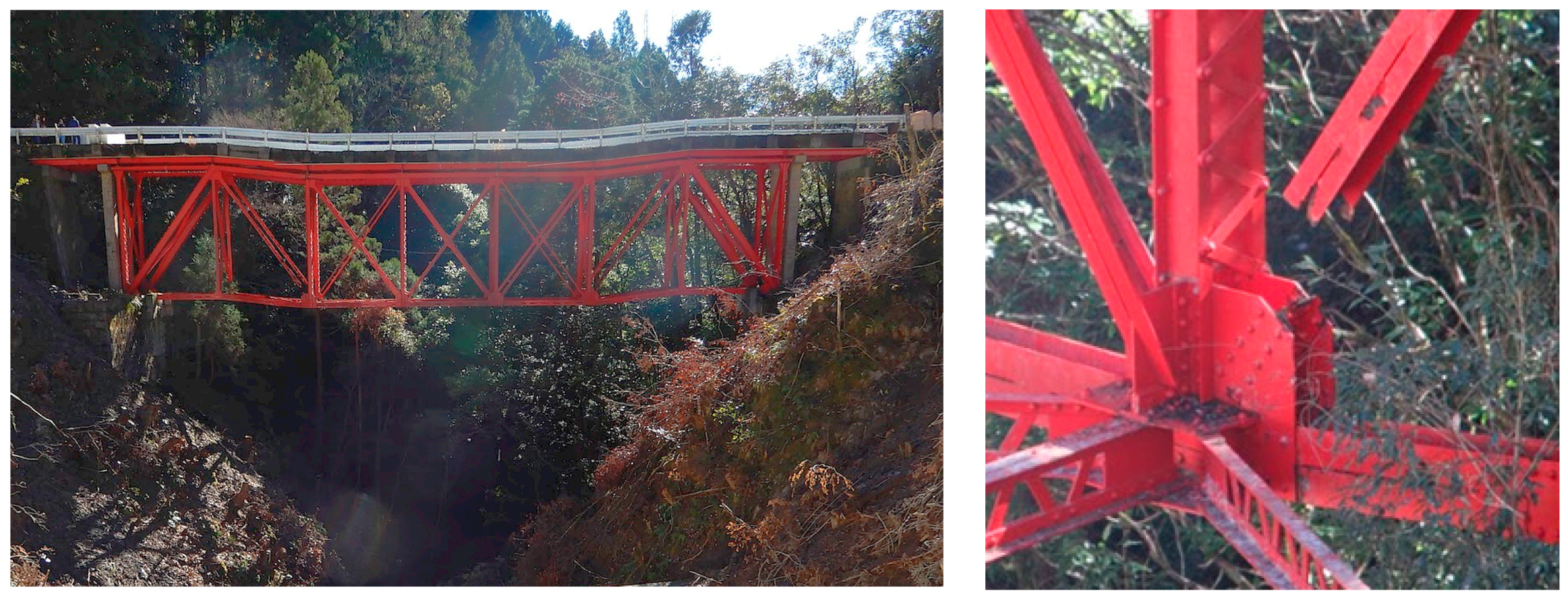
One example of the above is the 2016 Inubo Bridge case in Kochi Prefecture, where four-angled supports of a truss failed because of their load-bearing capacity being lowered by corrosion, causing the whole beam to become deformed (Figure 1). Corrosion was also a factor in the 2007 collapse of the I-35W Mississippi River Bridge in the United States [5]. Such accidents resulting from corrosion occur worldwide, and one of the causes for these accidents is an inability to accurately estimate the decline in strength caused by corrosion. In other words, a method to accurately assess lowered strength is required to inspect the safety of steel structures and determine the necessity for repair and/or reinforcement [6]. In much existing literature, the lowered strength is expressed by the term residual strength, and it is used in this paper [7,8,9].
The most anticipated method to improve the accuracy of residual strength evaluation is FEM analysis that accurately recreates the morphology of the corroded surface using solid elements. For example, it was showed that ANSYS (version 16.0, Canonsburg, PA, USA) solid elements can be used to accurately express mechanical behavior [9,10]. However, because the calculation cost is extremely high, this is not a realistic option for the analysis of civil engineering structures beyond experimental specimens. Thus, shell elements are usually used to reduce the calculation cost [11]. The average thickness is usually used to estimate the thickness of the shell element [12,13,14]; however, surface unevenness is known to have an impact on strength; thus, using only average thicknesses is not necessarily appropriate. Effective thickness as defined by Equation (1) is primarily considered appropriate to be used as the thickness of the shell element:
Thus, this study proposes a method that precisely estimates the effective thickness of the shell element from measurements of surface morphology. Although several methods have been proposed to obtain effective thickness from measurements of surface morphology [7,15,16], such thicknesses were estimated by manually selecting features such as the average thickness and standard deviation of thickness. Despite these features being important, the impact of surface morphology on strength is not sufficiently simple to be predictable from only a limited number of features. In other words, selecting or removing features manually is not desirable.
Therefore, we develop a method to estimate effective thickness based on deep learning. Deep learning is a type of machine learning that uses multilayered neural networks, which have attracted attention in recent years and is characterized by its ability to automatically obtain many ideal features during the learning process. We particularly used a convolutional neutral network (CNN), which displays high performance in terms of image analysis, even for deep learning. Although the input to the CNN was surface morphology converted to images, the output was an effective thickness as defined in Equation (1). Thus, analyses can be performed without removing necessary features through manual selection.
To train CNN and improve its performance, a large training dataset with paired input and teaching output is necessary. However, performing loading tests sufficient to obtain enough data for deep learning is impossible. Thus, we performed FEM analyses in which the surface morphology was changed in multiple ways to accumulate data. If CNN is trained appropriately in this manner, the effective thickness of shell elements can be precisely estimated even when a new corrosion morphology, i.e., one that was not used during learning, is given to CNN.
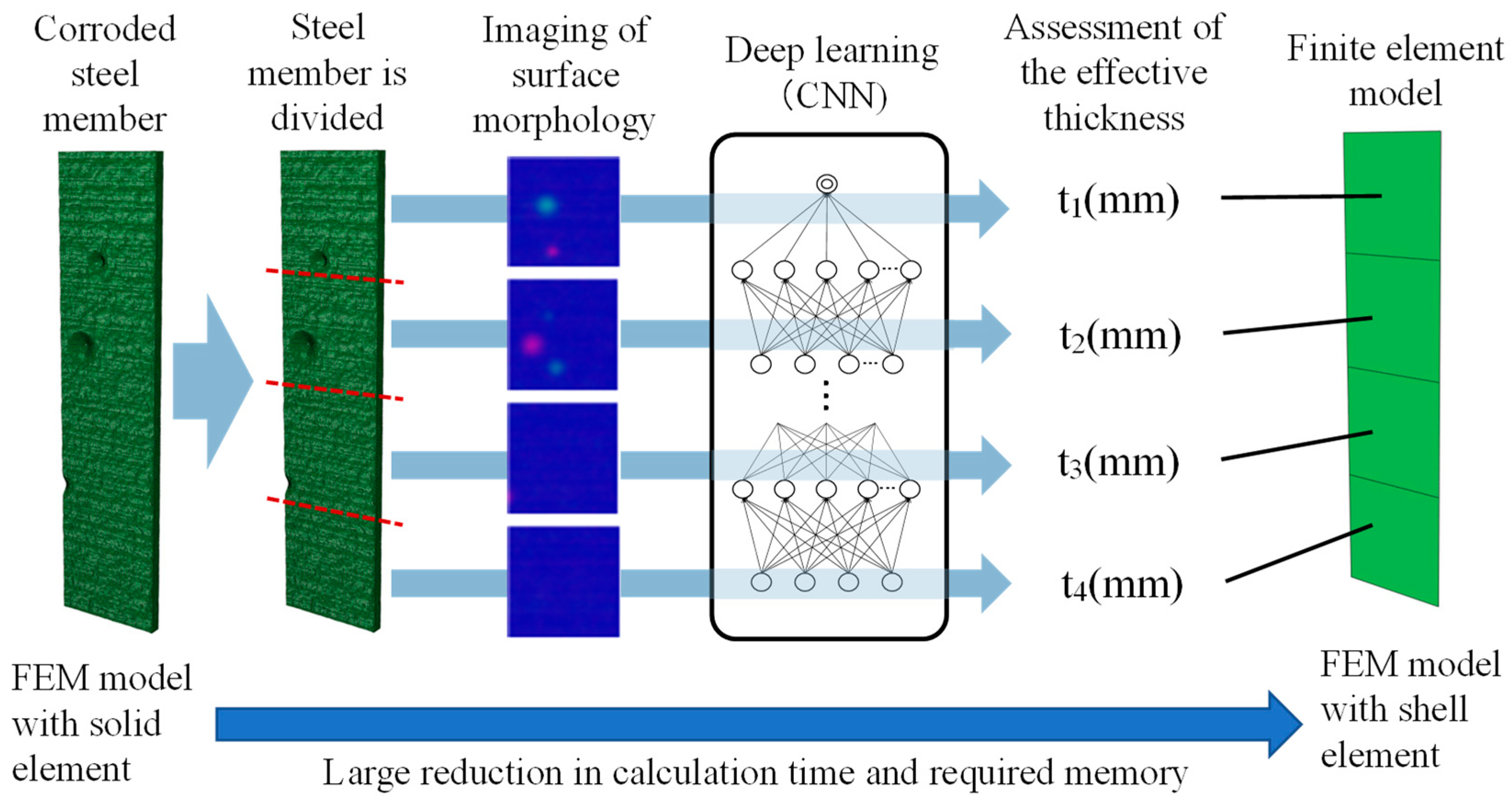
Because this approach improves the precision of each element in steel structural members with corrosion, a FEM model with high precision can be designed for the overall structure. Figure 2 shows the developing flow of the proposed FEM model using a steel plate as an example. First, a steel structural member was divided into several elements (corroded steel fragments), and the surface morphology of each of these corroded fragments was visualized. This image was then provided to CNN to assess the effective thickness of the corroded steel fragment. Next, this effective thickness was used to build a shell element model for analysis, shown on the right-hand side of Figure 2. As an example of a corroded steel structural member, we analyzed corroded steel plates and H-section steel under tension by converting to a shell element model with the method shown in Figure 2. The result was compared with the solid element model to verify its validity.
2. Accumulation of Learning Data through FEM Analysis
2.1. Verifying the Validity of the FEM Model
In this study, we performed CNN learning using the FEM analytical results with solid elements for multiple numerically generated corroded steel fragments. To that end, it was first necessary to confirm that the mechanical behavior of the corroded steel member was appropriately recreated using FEM. Ideally, we should learn from the tensile test results of actual corroded steel fragments instead of the FEM analytical result, but the number of learning data is too small; therefore, the FEM analysis was used.
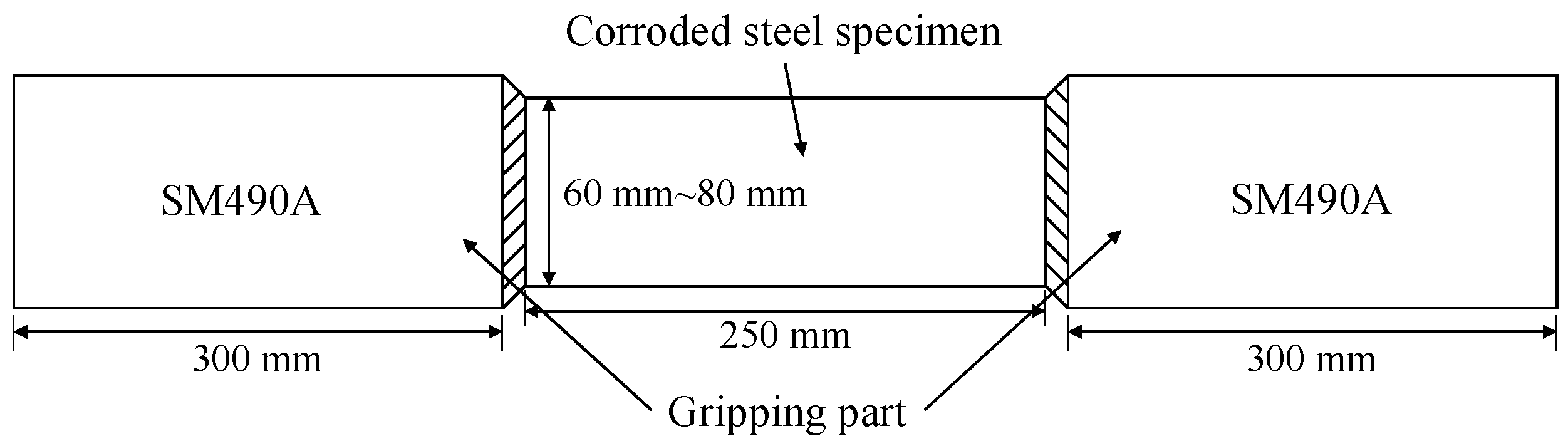
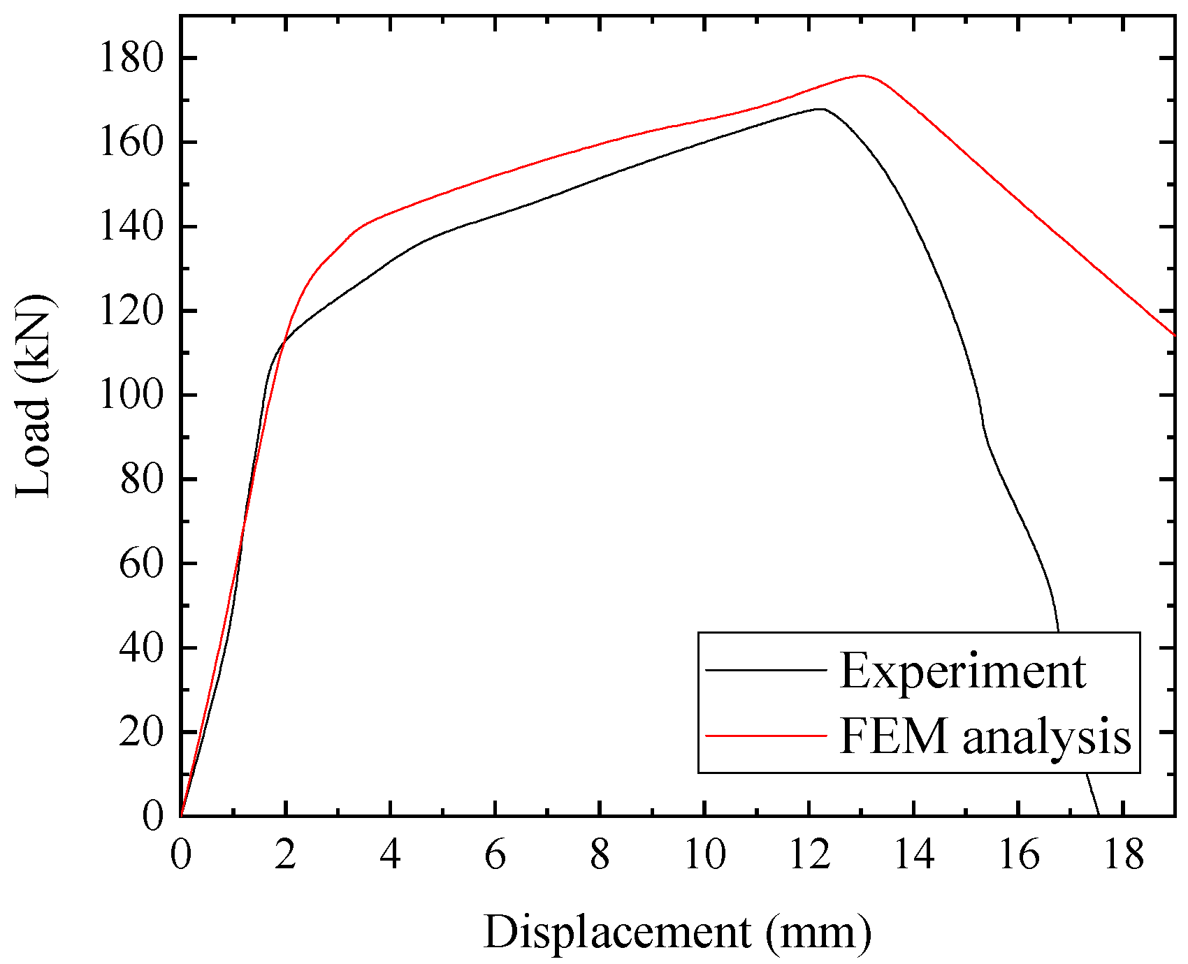
We used the commercially available FEM analytical package (Abaqus/Standard) to confirm that the tensile test result acquired from two corroded steel beams could be precisely recreated using the FEM analysis with the solid element C3D8 (i.e., 3D 8-node hexahedral elements) [17]. Specimen dimensions in the experiment are illustrated in Figure 3, the measurement system for surface morphology is illustrated in Figure 4, and the experimental conditions are illustrated in Figure 5. A total of 30 specimens were constructed from the obtained material, and results that compared its maximum load are illustrated in Figure 6. A comparison between the sample after failure and the FEM-based Mises stress distribution are illustrated in Figure 7, and the load-displacement curve is illustrated in Figure 8. As seen in Figure 7, the average error was 4.7%, and only one specimen had an error exceeding 10% wherein stresses at the point of failure are higher. In addition, the load-displacement curve in Figure 8 accurately recreates the experimental results, and the failure mode of the corroded steel specimen is well represented using the FEM model.
2.2. Generation and Analysis of Corroded Steel Specimen Using a Spatial Autocorrelation Model
We artificially generated a FEM model for a corroded steel fragment using a spatial autocorrelation model and performed CNN learning using these FEM analytical results. The spatial autocorrelation model considers the correlation of the corrosion depth on a corroded surface created with a feature of unevenness comprising both depth and width. This model was formulated as in Equation (2), and the corrosion distribution was derived from this Equation.
where Vi’ is the corrosion depth at the ith measurement point, Vi is the independent corrosion depth at the ith measurement point, β is the distance attenuation coefficient, and dij is the distance between point i and point j. We considered the examination by Okumura et al. [18] and randomly chose β between 0.28 and 0.4 for each specimen. For the independent corrosion depth, we used randomly generated numbers according to the Poisson distribution, and the initial thickness was randomly determined to have a range of 8–25 mm. As above, all the values of the right side are determined, and the left side is obtained by the calculation of Equation (2). Additionally, to recreate pitting, we created elliptical regions of damage, each of which had a random radius between 5 mm and 15 mm. The thickness was generated using a 2-mm mesh. It has been confirmed in [15,16,17] that the mechanical behavior can be reproduced by such expression of the mm order.
Figure 9 shows an example FEM model of a corroded steel fragment generated in this manner. We randomly determined the height and width of the fragment in the range of 126–254 mm and generated a total of 10,000 fragments. However, because the mesh size was set at 2 mm, the length was set in multiples of 2 mm to prevent meshes with sizes between these intervals.
The relation between true stress and true strain for the material was found to be trilinear (Figure 10), with Young’s modulus E of 2.05 × 10⁵ MPa, Poisson’s ratio ν of 0.3, yield stress σy of 245 MPa, and ultimate strength σu of 400 MPa. We performed a tensile analysis on the corroded steel fragments generated in this manner and obtained their effective thickness according to Equation (1). These results were used for the deep learning described in the next section.
3. Building a Model to Assess Effective Thickness Using Deep Learning
3.1. Outline of CNN
We created a method to assess effective thickness using CNN, which is a type of deep learning. CNN models the receptive field in the human field of vision and is known to have a high level of performance in the field of image recognition. We present the outline of CNN below considering the convenience of readers; more detail regarding the approach can be found in previous studies [19,20].
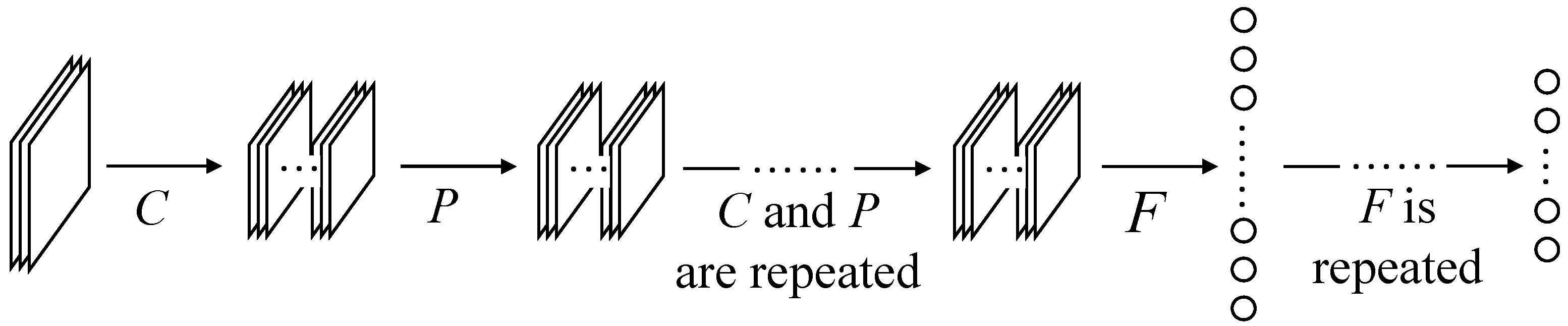
CNN differs from the conventional neural network and is characterized by two special layers: the convolutional layer and the pooling layer. Figure 11 shows a typical CNN structure. First, an image is added to the input layer, followed by repeated calculations in the convolutional and pooling layers. In the fully connected layer, a weighted connection calculation similar to a conventional neural network is performed. The classification result is outputted in the output layer.
3.1.1. The Convolutional Layer
The convolutional layer runs an operation in which filters are convoluted for the provided input; thus, this layer identifies localized characteristics. Assuming that the size of images inputted to the convolutional layer is W × H × K, the size of the filter is given by w × h × K × L. W is the image width, H is the image height, K is the number of channels of the image inputted to the convolutional layer, w is the width of the filter, h is the height of the filter, and L is the number of filters.
If the pixel value of the input image is expressed using xijk with the index (i, j) (i = 0, …, W − 1, j = 0, …, H − 1, k = 1, …, K) and the pixel value of the filter using hpqkl (l = 1, …, L) with the index (p, q) (p = 0, …, w − 1, q = 0, …, h − 1), the convolution operation is expressed with Equation (3):
where uijl is the pixel number of the output image and bl is bias.
Next, we applied the activation function f to uijl obtained with Equation (3) as shown in Equation (4):
Activation function, such as the sigmoid function, tanh, a normalized linear function called ReLU (Rectified Linear Unit), and softsign functions have all been proposed previously; in this research, we used ReLU, which has been reported to be the best-suited [19]. ReLU is expressed using Equation (5):
Output images obtained from these analyses are used as the input for the next layer.
3.1.2. The Pooling Layer
The pooling layer is usually placed immediately after the convolutional layer and by lowering the positional sensitivity of the filter response obtained in the convolutional layer, invariance against microscopic horizontal changes can be achieved. The pooling layer obtains a representative value for a part of the group of pixels in the input image and uses this value as the pixel value for the new output image. In image analysis, considering the maximum pooling that uses the maximum value as the representative value is common. We used this approach in the present study.
3.1.3. The Fully Connected Layer and the Output Layer
The provided input image is one-dimensionally operated in the fully connected layer and all input and output units are connected. This point is the difference between the convolutional layer and the pooling layer wherein only specified nodes are connected. In the final output layer, the effective thickness is output as a continuous value, and learning is performed such that the sum of the squared errors for the output and the target output (output provided as the teacher) would be minimum values. In this manner, an ideal weight can be obtained.
3.2. Generation of Input Image for CNN and Learning
In the previous section, we discussed the outline of CNN and introduced the advantage of superior image recognition. To use this advantage, the morphology of the corroded surface was imaged and used as the input for CNN. The generated image was a 3-channel RGB color image, where the R, G, and B channels were given front surface thickness reduction, back surface thickness reduction, and an initial thickness, normalized to 25 mm, which is the possible maximum initial thickness of the model stipulated in Section 2.2. Considering that the thickness was generated with a 2-mm mesh, e.g., if the width was x mm, the pixel number in the width was set as x/2 + 1.
The image of a case with notable pitting (Figure 9a) is shown on the left-hand side of Figure 12. The pit near the center of the front surface (top image in Figure 9a) led to high thickness reduction at the center, increasing the R channel value and creating a red circle at the center of the left image in Figure 12. In contrast, the image of a case with average corrosion (Figure 9b), shown on the right side of Figure 12, has similar pixel numbers throughout the image because there is no location with notable thickness reduction as in Figure 9a.
3.3. Proposed Feature Extraction Layer
In Section 3.1, we explained the outline of CNN and basic layers. In this study, we set a layer that extracts characteristics that are considered effective to improve precision based on domain knowledge along with these basic layers. In particular, the length, width, average thickness, standard deviation of thickness, minimum thickness, and average thickness of the minimum cross-section of the steel plate were calculated. Information pertaining to the length and width of the steel fragment are lost during the deformation of the image to 256 × 256 pixels and were thus secured at this point. The average thickness, standard deviation of thickness, minimum thickness, and average thickness of the minimum cross-section are insufficient indexes in terms of precision to evaluate the effective thickness alone but were thought effective when assessing the effective thickness in combination with other indexes.
3.4. CNN Learning and Verification of the Model Precision
In this section, we create CNN with the image created in Section 3.2 as input and the effective thickness obtained from the load-bearing capacity determined in the FEM analysis in Section 2 as output. Figure 13 shows the schematic. First, as shown in the frame entitled “Training Datasets” in Figure 13, many images and the related data of the effective thickness are used as the learning data. Next, based on these data, CNN learning is performed. This allows for the effective thickness for the new image (the top of the “Analysis Stage”) not used for the training stage to be obtained with good precision.
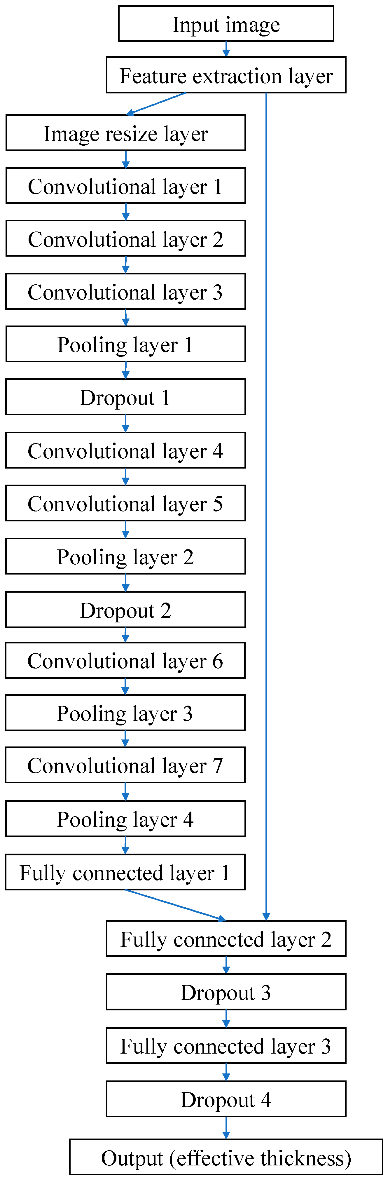
Figure 14 shows the structure of CNN created for this study. The number of filters, size, and output images for each layer are shown in Table 1. The feature extraction layer calculates six features discussed in Section 3.3 from input images. This is then followed by deformation of input images to 256 × 256 pixels in the image resize layer. Similar to the basic CNN, the convolutional layer and the pooling layer are repeated, and in the fully connected layer, six features identified in the feature extraction layer are connected. However, in between the top layers, the convolutional layers are mainly used without the pooling layer in between. If the pooling layer is used when the number of convolutions by the convolutional layers is small, information on small unevenness is lost, thereby reducing the precision.
Conventional CNN used for the classification often used a method in which nodes were prepared for the number of classes in the output layer, and classes were determined based on the SoftMax function. However, in this study, because the objective was regression (predicting the continuous value: effective thickness) instead of classification, the final layer was one node and the effective thickness appeared.
To verify the precision of regression, we performed K-fold cross-validation. K-fold cross-validation classifies samples into K group, and uses samples in the K − 1 group for learning. This learning result is used to analyze the remaining group. This is repeated K times. In this research, K was 10. The number of steel fragments analyzed was 10,000 as discussed in Section 2.2. The result is summarized in Figure 15. The horizontal axis shows the effective thickness calculated using Equation (1), whereas the vertical axis shows effective thickness assessed with CNN. The average error was 2.8%. The figure also shows that the effective thickness of the corroded steel fragment can be assessed with good precision.
4. FEM Modeling of Corroded Structural Members
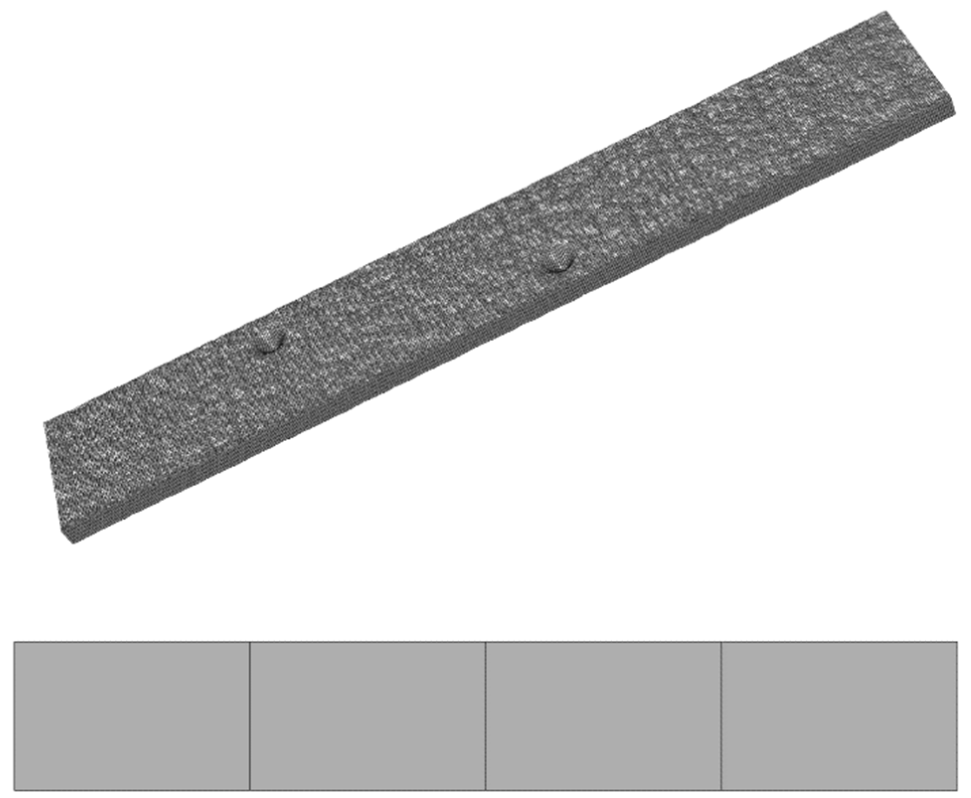
We created total a 400 sets, including 100 sets each of the FEM model with solid elements for the corroded steel plate and H-section steel, and that with shell elements, which uses the effective thickness assessment model created in the previous section, for the steel plate and H-section steel beam, and compared their tensile load-bearing capacity. Each FEM model was built based on the spatial autocorrelation model of Equation (2). Dimensions were as follows: for both the steel plate and H-section steel, the longitudinal length was between 120 mm to 1500 mm. Steel plate width was randomly determined between 128 mm and 256 mm, and flange and wave widths of the H-section steel were randomly determined between 128 mm and 300 mm. Please note that the minimum size is set to 128 mm to avoid being outside the learning range of the deep learning model built in Section 3. If it is necessary to reflect the size smaller than the learned range in the FEM model, it is necessary to expand the learning range of the deep learning model in Section 3. The present mesh generation method automatically generated the mesh so that the length of each element would be as close to 200 mm as possible. Figure 16 shows an example of the corroded steel plate and Figure 17 shows an example of the corroded H-section steel. Each Figure shows the solid element model on the top and the shell element model on the bottom.
Figure 18 shows the comparison of load-bearing capacity. It also shows the result of a model analysis that used shell element with the average thickness, which is the conventional method. Table 2 shows the relative error in each load-bearing capacity. Similar to the calculation used for the effective thickness, the average thickness was calculated with 2-mm mesh. As shown in Figure 18 and Table 2, the shell element model with the effective thickness clearly has higher precision when compared to the one with the average thickness.
Furthermore, when the average thickness was used, the strength of the shell element model tended to be higher than the strength of the solid element model. This is considered to be because of the stress concentration caused by uneven surface morphology cannot be accurately assessed when using the average thickness. This means overestimation of risk in the actual site, indicating that the present method is a superior method than ones that use the average thickness.
In addition, analytical time of the shell element model is notably shorter than that of the solid element model. For example, with the model in Figure 16, the analytical time for the solid element model was 1.04 × 10⁵ s, while the shell element model took 1.40 s. In all models, analytical time was 1/10,000 or less of that of the solid element model. In other words, we successfully reduced the calculation cost by a large margin while ensuring precision.
5. Conclusions
In this study, we appropriately evaluated the residual strength of corroded structural members under tension by assessing the effective thickness from the surface morphology using CNN and creating a FEM model that uses this effective thickness as the shell element thickness. In particular, when compared to a model that uses the average thickness, not only did the precision significantly improve but the tendency to overestimate the strength (i.e., dangerous side) also improved.
In the future, a model that can assess shearing and buckling together with tension needs to be created. By applying the present method, creating such a model is possible, and a study is under way. In this manner, the buckling of a steel pier due to corrosion can be evaluated [21].
Additionally, we predicted the residual strength by visualizing the damage to corroded structural members and using it as an input to CNN. Application of CNN is not limited to corroded structural members. In other words, the present result indicates that the mechanical behavior of other structures can be predicted by visualization, and we will continue to apply the present method to analyze a wider range of structures.
Author Contributions
Conceptualization, P.-j.C. and T.K.; Formal analysis, P.-j.C., T.Y. and S.I.; Investigation, P.-j.C. and T.Y.; Methodology, T.K.; Writing—original draft, P.-j.C.; Writing—review & editing, P.-j.C.
Funding
This research received no external funding.
Conflicts of Interest
The authors declare no conflict of interest.
References
- Krechkovska, H.; Student, O.; Lesiuk, G.; Correia, J. Features of the microstructural and mechanical degradation of long term operated mild steel. Int. J. Struct. Integr. 2018, 9, 296–306. [Google Scholar] [CrossRef]
- Lesiuk, G.; Rymsza, B.; Rabiega, J.; Correia, J.A.; De Jesus, A.M.P.; Calcada, R. Influence of loading direction on the static and fatigue fracture properties of the long term operated metallic materials. Eng. Fail. Anal. 2019, 96, 409–425. [Google Scholar] [CrossRef]
- Liu, Z.; Hebdon, M.H.; Correia, J.A.; Carvalho, H.; Vilela, P.M.; de Jesus, A.M.; Calçada, R.A. Fatigue assessment of critical connections in a historic Eyebar suspension bridge. J. Perform. Constr. Facil. 2018, 33, 04018091. [Google Scholar] [CrossRef]
- Lesiuk, G.; Correia, J.; Smolnicki, M.; De Jesus, A.; Duda, M.; Montenegro, P.; Calcada, R. Fatigue Crack Growth Rate of the Long Term Operated Puddle Iron from the Eiffel Bridge. Metals 2019, 9, 53. [Google Scholar] [CrossRef]
- National Transportation Safety Board. Collapse of I-35W Highway Bridge, Minneapolis, Minnesota, August 1, 2007; Highway Accident Report NTSB/HAR-08/03; National Transportation Safety: Washington, DC, USA, 2008.
- Kariya, A.; Tagaya, K.; Kaita, T.; Fujii, K. Mechanical properties of corroded steel plate under tensile force. In Proceedings of the 3rd International Structural Engineering and Construction Conference (ISEC-03), Shunan, Japan, 20–23 September 2005; Hara, T., Ed.; CRC Press: Boca Raton, FL, USA, 2005; pp. 105–110. [Google Scholar]
- Kim, I.T.; Dao, D.K.; Jeong, Y.S.; Huh, J.; Ahn, J.H. Effect of corrosion on the tension behavior of painted structural steel members. J. Constr. Steel Res. 2017, 133, 256–268. [Google Scholar] [CrossRef]
- Appuhamy, J.M.R.S.; Ohga, M.; Chun, P.; Dissanayake, P.B.R. Numerical investigation of residual strength and energy dissipation capacities of corroded bridge members under earthquake loading. J. Earthq. Eng. 2013, 17, 171–186. [Google Scholar] [CrossRef]
- Wang, Y.; Xu, S.; Wang, H.; Li, A. Predicting the residual strength and deformability of corroded steel plate based on the corrosion morphology. Constr. Build. Mater. 2017, 152, 777–793. [Google Scholar] [CrossRef]
- Qin, G.C.; Xu, S.H.; Yao, D.Q.; Zhang, Z.X. Study on the degradation of mechanical properties of corroded steel plates based on surface topography. J. Constr. Steel Res. 2016, 125, 205–217. [Google Scholar] [CrossRef]
- Sultana, S.; Wang, Y.; Sobey, A.J.; Wharton, J.A.; Shenoi, R.A. Influence of corrosion on the ultimate compressive strength of steel plates and stiffened panels. Thin-Walled Struct. 2015, 96, 95–104. [Google Scholar] [CrossRef]
- Tung, N.X.; Nogami, K.; Yamamoto, N.; Yamasawa, T.; Yoda, T.; Kasano, H.; Murakoshi, J.; Toyama, N.; Sawada, M. Measurement of Corroded Gusset Plate Connection of Steel Truss Bridge and Evaluation for its Corrosion State. In Design, Fabrication and Economy of Metal Structures; Springer: Berlin/Heidelberg, Germany, 2013; pp. 657–662. [Google Scholar]
- Nguyen, X.T.; Nogami, K.; Yoda, T.; Kasano, H.; Murakoshi, J.; Sawada, M. Evaluation of corrosion state of gusset plate connections of steel truss bridge. Kou kouzou rombunshuu 2014, 21, 71–83. [Google Scholar]
- Chun, P.J.; Yamashita, H.; Furukawa, S. Bridge damage severity quantification using multipoint acceleration measurement and artificial neural networks. Shock Vib. 2015, 2015, 1–11. [Google Scholar] [CrossRef]
- Appuhamy, J.R.S.; Ohga, M.; Kaita, T.; Dissanayake, R. Reduction of ultimate strength due to corrosion-A finite element computational method. Int. J. Eng. 2011, 5, 194. [Google Scholar]
- Kaita, T.; Appuhamy, J.M.R.S.; Itogawa, K.; Ohga, M.; Fujii, K. Experimental study on remaining strength estimation of corroded wide steel plates under tensile force. Procedia Eng. 2011, 14, 2707–2713. [Google Scholar] [CrossRef]
- Karina, C.N.; Chun, P.J.; Okubo, K. Tensile strength prediction of corroded steel plates by using machine learning approach. Steel Compos. Struct. 2017, 24, 635–641. [Google Scholar]
- Okumura, M.; Fujii, K.; Tukai, M. Statistical model of steel corrosion considering spatial auto-correlation. Doboku Gakkai Ronbunshu 2001, 2011, 109–116. [Google Scholar] [CrossRef]
- LeCun, Y.; Bengio, Y.; Hinton, G. Deep learning. Nature 2015, 521, 436–444. [Google Scholar] [CrossRef] [PubMed]
- Goodfellow, I.; Bengio, Y.; Courville, A. Deep Learning; MIT Press: Cambridge, MA, USA, 2016. [Google Scholar]
- Chun, P.J.; Tsukada, K.; Kusumoto, M.; Okubo, K. Investigation and repair plan for abraded steel bridge piers: case study from Japan. Proc. Inst. Civ. Eng. -Forensic Eng. 2019, 172, 11–18. [Google Scholar] [CrossRef]
Figure 1.
Deformation of the Inubo Bridge. (Left: overall view of the bridge. Right: detail of the broken structural member.).
Figure 1.
Deformation of the Inubo Bridge. (Left: overall view of the bridge. Right: detail of the broken structural member.).

Figure 2.
Developing of the FEM model proposed.

Figure 3.
Dimensions of the corroded steel specimen. (SM 490A is a steel material determined by the Japanese Industrial Standards).
Figure 3.
Dimensions of the corroded steel specimen. (SM 490A is a steel material determined by the Japanese Industrial Standards).

Figure 4.
Measuring thickness using the 3D measuring device.

Figure 5.
Specimen prepared for tensile test.

Figure 6.
Comparison of tensile strength of Experimental and FEM results. The black line represents the 1:1 line between the experimental and FEM results, while the red and blue dotted lines indicate 5% and 10% overestimation/underestimation, respectively.
Figure 6.
Comparison of tensile strength of Experimental and FEM results. The black line represents the 1:1 line between the experimental and FEM results, while the red and blue dotted lines indicate 5% and 10% overestimation/underestimation, respectively.

Figure 7.
An example of FEM analysis stress distribution compared with the failure of the steel plate.
Figure 7.
An example of FEM analysis stress distribution compared with the failure of the steel plate.

Figure 8.
Comparison results between experimental and FEM results.

Figure 9.
FEM models for corroded steel fragments prepared based on the spatial autocorrelation model. For each case, the front and back surfaces are shown.
Figure 9.
FEM models for corroded steel fragments prepared based on the spatial autocorrelation model. For each case, the front and back surfaces are shown.

Figure 10.
Stress–strain curve used for the analysis.

Figure 11.
Basic structure of CNN (C = convolutional layer, P = pooling layer, and F = fully connected layer).
Figure 11.
Basic structure of CNN (C = convolutional layer, P = pooling layer, and F = fully connected layer).

Figure 12.
An image of the steel fragment from Figure 9. (The left image shows a case with visible pitting, whereas the right image shows a case with average corrosion).
Figure 12.
An image of the steel fragment from Figure 9. (The left image shows a case with visible pitting, whereas the right image shows a case with average corrosion).

Figure 13.
Overview of the learning process.

Figure 14.
The overall structure of CNN used in the present study.

Figure 15.
Verification of the precision in the effective thickness assessment.

Figure 16.
A model of corroded steel specimen (in this example, dimensions are as follows: width = 128 mm, length = 810 mm, and initial thickness = 10 mm).
Figure 16.
A model of corroded steel specimen (in this example, dimensions are as follows: width = 128 mm, length = 810 mm, and initial thickness = 10 mm).

Figure 17.
A model for corroded H-section steel (in this case, dimensions are as follows: flange width = 160 mm, wave height = 140 mm, longitudinal length 1400 mm, and thickness = 10 mm).
Figure 17.
A model for corroded H-section steel (in this case, dimensions are as follows: flange width = 160 mm, wave height = 140 mm, longitudinal length 1400 mm, and thickness = 10 mm).

Figure 18.
Comparison of load-bearing capacity for the shell element model with the effective thickness, the shell element model with average thickness, and solid element model.
Figure 18.
Comparison of load-bearing capacity for the shell element model with the effective thickness, the shell element model with average thickness, and solid element model.


Table 1.
Filter and output image size for each layer.
| Layer Name | The Number of Filters | Size or Dropout Rate | Output Size |
|---|---|---|---|
| Input image | - | - | Original image size |
| Feature extraction layer | - | - | Original image size |
| Image resize layer | - | - | 256 × 256 × 3 |
| Convolutional layer 1 | 32 | 11 × 11 | 246 × 246 × 32 |
| Convolutional layer 2 | 32 | 7 × 7 | 240 × 240 × 32 |
| Convolutional layer 3 | 32 | 3 × 3 | 238 × 238 × 32 |
| Pooling layer 1 | - | 2 × 2 | 119 × 119 × 32 |
| Dropout 1 | - | 0.2 | 119 × 119 × 32 |
| Convolutional layer 4 | 64 | 7 × 7 | 113 × 113 × 64 |
| Convolutional layer 5 | 64 | 3 × 3 | 111 × 111 × 64 |
| Pooling layer 2 | - | 2 × 2 | 55 × 55 × 64 |
| Dropout 2 | - | 0.2 | - |
| Convolutional layer 6 | 128 | 5 × 5 | 53 × 53 × 128 |
| Pooling layer 3 | - | 2 × 2 | 26 × 26 × 128 |
| Convolutional layer 4 | 256 | 3 × 3 | 24 × 24 × 256 |
| Pooling layer 4 | - | 2 × 2 | 12 × 12 × 256 |
| Fully connected layer 1 | - | - | 200 |
| Fully connected layer 2 | - | - | 40 |
| Dropout 3 | - | 0.2 | - |
| Fully connected layer 3 | - | - | 20 |
| Dropout 4 | - | 0.2 | - |
| output | - | - | 1 |
Table 2.
Mean relative error in load-bearing capacity between the effective thickness model, average thickness model, and solid element model.
Table 2.
Mean relative error in load-bearing capacity between the effective thickness model, average thickness model, and solid element model.
| Model Type | Effective Thickness Model | Average Thickness Model |
|---|---|---|
| Steel plate model | 3.3% | 22.0% |
| H-section steel model | 4.2% | 16.8% |
© 2019 by the authors. Licensee MDPI, Basel, Switzerland. This article is an open access article distributed under the terms and conditions of the Creative Commons Attribution (CC BY) license (http://creativecommons.org/licenses/by/4.0/).
Share and Cite
MDPI and ACS Style
Chun, P.-j.; Yamane, T.; Izumi, S.; Kameda, T. Evaluation of Tensile Performance of Steel Members by Analysis of Corroded Steel Surface Using Deep Learning. Metals 2019, 9, 1259. https://doi.org/10.3390/met9121259
AMA Style
Chun P-j, Yamane T, Izumi S, Kameda T. Evaluation of Tensile Performance of Steel Members by Analysis of Corroded Steel Surface Using Deep Learning. Metals. 2019; 9(12):1259. https://doi.org/10.3390/met9121259
Chicago/Turabian StyleChun, Pang-jo, Tatsuro Yamane, Shota Izumi, and Toshihiro Kameda. 2019. "Evaluation of Tensile Performance of Steel Members by Analysis of Corroded Steel Surface Using Deep Learning" Metals 9, no. 12: 1259. https://doi.org/10.3390/met9121259
Note that from the first issue of 2016, this journal uses article numbers instead of page numbers. See further details here.