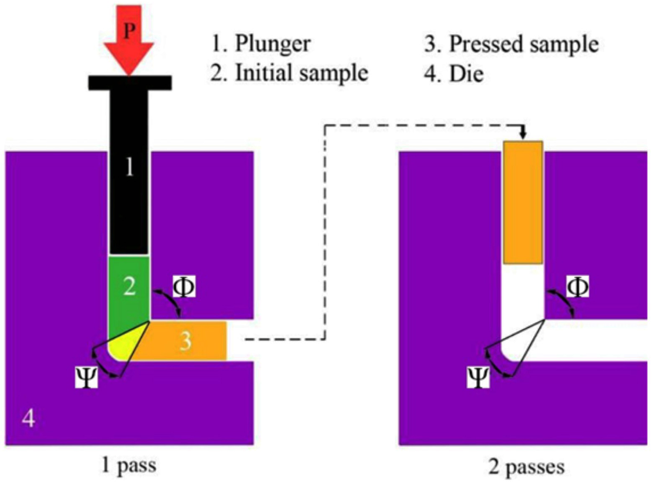
3.1. Process Operation Design
We shall consider the problem of designing the operation of cutting the aluminum workpiece as a hill-climbing problem in a vector space with Cartesian coordinates. In practice, the target function of this problem has several local minima in the feasibility region. There is certainly a need to find the global minimum or maximum in such studies.
The most promising method for solving these sorts of problems are dedicated search algorithms based on random strategies [
58,
59,
60] and the projection of the informational bases of biological systems onto computing technologies. The most popular are currently ANN and genetic algorithms; both methods are effective in the field of local strategies and, most importantly, both provide the opportunity of exiting these fields during a global search.
Quality research requires a clear understanding of both the methodology and the research process. Experimental computer-based studies in the form of experimental simulations generally use multi-step methods. Graphical approaches to the target function surface used for this purpose build up graphical images and provide a reasonable representation of the computational experiment.
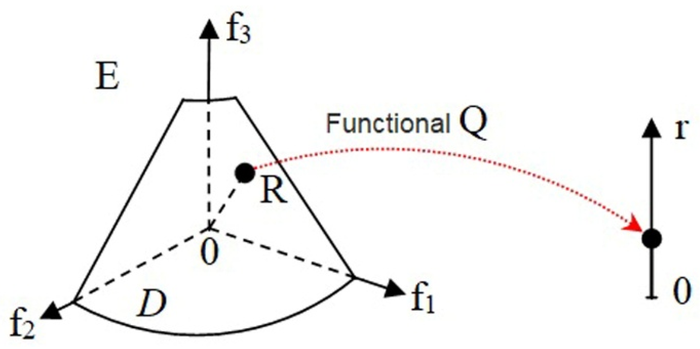
The mathematical procedure for system adaptation is essentially the investigation of a target function minimization problem in a certain convex area, D, of a normalized variable space, E. The target function is based on a convex numeric function or Q function that transposes area D onto a set of non-negative numbers. In the cutting tool-workpiece system adaptation problem, Q will determine the distance, r, between the point of convex area, D, and the origin of the coordinates of the normalized optimization criteria and the length of the vector, OR, in a non-negative multiobjective space E (
Figure 4).
Technical systems are steadily becoming more complex and the solutions to adaptation problem need complex setups for complicated control problems. Hence, modern adaptive systems must be complemented by artificial neural structures.
Firstly, the algorithm that calculates the optimum cutting parameters must be defined. A multicriterion optimization problem is initially set up, defining the criteria, the limitations, and the boundary conditions. The relationship is established between the machining parameters and the product parameters and the microstructure, employing a neural network to approximate the experimental data. A graphical interpretation of the surface of a normalized three-dimensional space is then created and the system states are determined, in which the values of each particular index cannot be improved without impairing the others, i.e., the Pareto frontier. In conclusion, the optimal workpiece turning conditions are defined that depend on both the physical and the mechanical properties of the alloy.
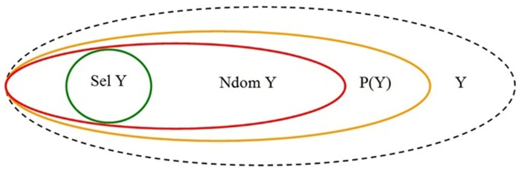
The following nomenclature is used: DM—decision maker; m—number of criteria; I = {1, 2, …, m}—set of criterion numbers; X—set of possible decisions; f = (f1, f2, …, fm)—vector-valued criterion; Y = f(X)—set of possible vectors (estimates); Rm—Euclidean space of m-dimensional vectors with real components; >X—preference relation of DM specified in the set Х; >Y—preference relation of DM, induced on the set with >X and specified in the set Y; >—relation > Y continued in the entire set Rm; Sel X—set of selected decisions; Sel Y—set of selected vectors (estimates); Ndom X—set of non-dominated decisions; Ndom Y—set of non-dominated vectors (estimates); Pf(X)—set of Pareto optimal decisions; P(Y)—set of Pareto-optimal vectors (Pareto optimal estimates).
Graphically, the correlation of sets of vector estimates in a multiobjective environment is shown in
Figure 5.
3.2. Formulation of an Optimization Problem
The objective of the investigation of the machining operation implies the following optimization problem criteria: f1—surface roughness (Ra, μm) and f2—machining time for unit volume removal in one cutting tool pass (Tm, min/cm3), and f3—the cost price of processing one part (C, $), i.e., m = 3. Relatively, a set of possible Y estimates in the three-dimensional space, R3, is formed with vectors f = (f1, f2, f3). A search is then performed for a set of estimates having the minimum length of vector f, which is a vector from the origin of coordinates to a point on the estimate surface. Let us present the criteria in a normalized dimensionless form with the index 1 assigned to the maximum actual numbers.
The test system varied the parameters in accordance with the following experimental table (see
Table 2):
х1 = [100 ÷ 200]—cutting speed,
vc, m/min;
х2 = [0.1 ÷ 0.4]—depth of cut,
ap, mm;
х3 = [0.012 ÷ 0.15]—feed,
fr, mm/rev.
The state of the system was evaluated through four criteria (
Table 5,
Table 6,
Table 7 and
Table 8). The first criterion was surface roughness,
Ra (µm), or dimensionless surface roughness,
Ra*(
f1); the second criterion was the unit volume machining time,
Tm (min/cm
3), or the dimensionless unit volume machining time,
Tm*(
f2). The third criterion was the cost price of processing one part,
C ($), or the dimensionless cost price of processing one part,
C*(
f3). The fourth criterion was the dimensionless vector of estimates in a three-dimensional normalized space,
f.
The values of the first criterion were taken from the experimental table and the rest were calculated on the basis of Formulas (3)–(8)
where
Tm is the machining time in turning,
T/ = (
L +
l1)/(
n ·
fr), where spindle speed
n = (1000 ·
vc)/(3.141 ·
d);
L is machining length section;
l1 is allowance length;
d is diameter of cut.
where,
is surface roughness for the current combination of X... and
fr;
Ramax is the maximum surface roughness value of all the
vc, ap, and
fr combinations;
Tm i is the unit-volume machining time for the current values of
vc, ap, and
fr;
Tm max is the maximum unit-volume machining time of all the
vc, ap, and
fr combinations;
Сi is the cost price of processing one part for the current combination of
vc, ap, and
fr; and
Ci max is the maximum value.
The optimum search procedure involves a non-negative set of vector estimates and it eliminates the variation of parameter values below zero. The boundary condition is, therefore, that all the variables in this model are non-negative.
Now that the optimization problem is formulated, we shall build and train the four neural networks that should become the operators both for the functions of the three variables, f(x1, x2, x3) and f(f1, f2, f3), and for the Q functions on the planes, f(f1, f2, f3). The complex ANN was constructed using the Skif AURORA-SUSU supercomputer cluster (South Ural State University, Chelyabinsk, Russia).
3.3. Building a Neural Network
Matlab is a leading software package, from among other mathematical software—Maple, Mathematica and Mathcad—designed for versatile numeric calculations of fundamental quality. The Neural Network Toolbox in Matlab, designed to create models and to train them, facilitates neural network creation. An undeniable advantage of Matlab is its language, with which users can create their own algorithms and applications. The versatility of the language provides opportunities for accomplishing a number of tasks such as collecting, analyzing, and structuring data, developing algorithms, modeling systems, object-oriented programming, development of a graphical user interface, debugging and converting Matlab applications to C or C++ code. Hence, the programming environment of choice, which is Matlab R2010b (parallel processing version).
The controlled feedforward neural network in the form of a multilayer perceptron (MLP) was trained with the Levenberg–Marquardt algorithm. The network structure was embedded in a hidden layer of sigmoid neurons and a linear layer of output neurons, which is the best structure for multidimensional mapping problems.
Only the normalized values with respect to the maximum were used for training the network. They were limited to the [0.1] range that improved the efficiency of the training.
Improvements to the generalization performance of the network solved the overfitting problem. Two data sets were used to do so: the training set that updated weights and offsets, and the validation set that stops the training when an undesirable event occurs.
The final configuration (the number of neurons in the hidden layer) of the network will be established based on the lowest mean squared error of the validation set.
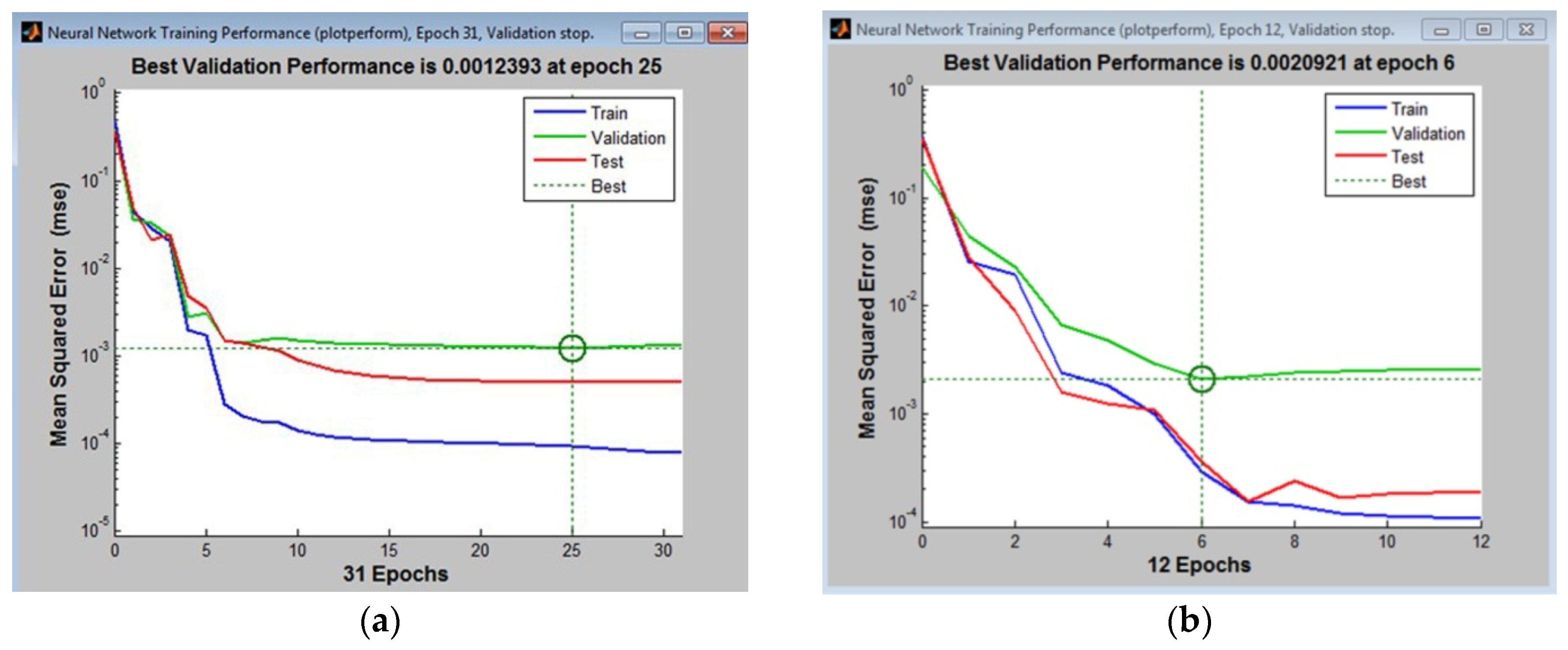
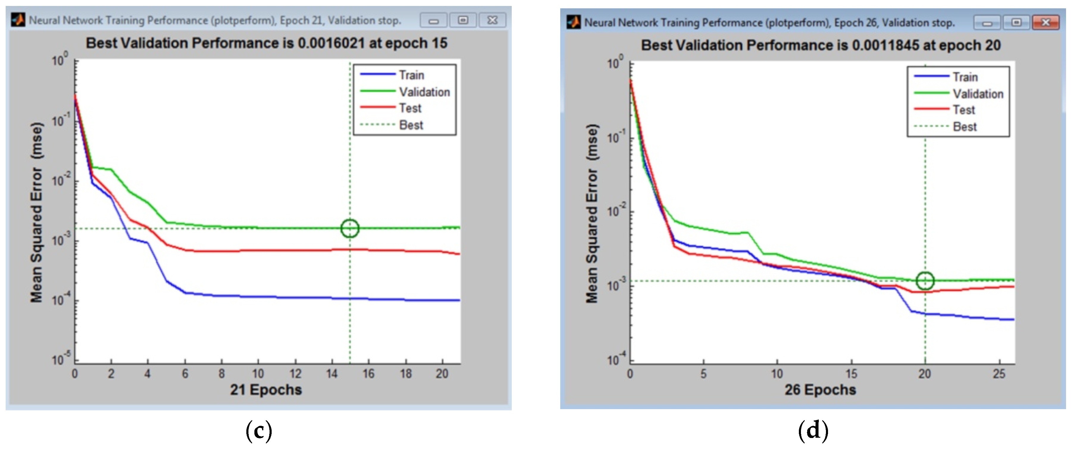
The multilayer perceptrons were, to begin with, trained with nine, 10, and 11 neurons in the hidden layer, with 15% of the tabular data allocated to the validation set. Having done the calculations for each of the hardening methods (ET500, ECAP-2, ECAP-4, ECAP-6), the lowest error values for MLP 3-10-4, presented in
Figure 6a–d were computed.
The coefficients of determination (
R2) with respect to criterion
f were 0.992 for the ET500 hardening method,
R2 = 0.956 for the ECAP-2 hardening method,
R2 = 0.988 for the ECAP-4 hardening method, and
R2 = 0.991 for the ECAP-6 hardening method, which reflects the high accuracy of the neural network prediction model ±0.8%, ±4.4%, ±1.9% and ±1.1%, respectively. The same structure appeared to be the best in generalization performance when 10% or 20% were allocated in the validation set of tabular data, shown in
Figure 6d. In the case of allocating 10% of the training set, the mean square errors of the networks were 0.0021 for the ET500 hardening method; 0.0032 for the ECAP-2 hardening method; 0.0022 for the ECAP-4 hardening method; 0.0045 for the ECAP-6 hardening method, and in the case of allocating 15% the mean square errors of the networks were 0.0018 for the ET500 hardening method; 0.0028 for the ECAP-2 hardening method; 0.0019 for the ECAP-4 hardening method; and 0.0031 for the ECAP-6 hardening method, respectively.
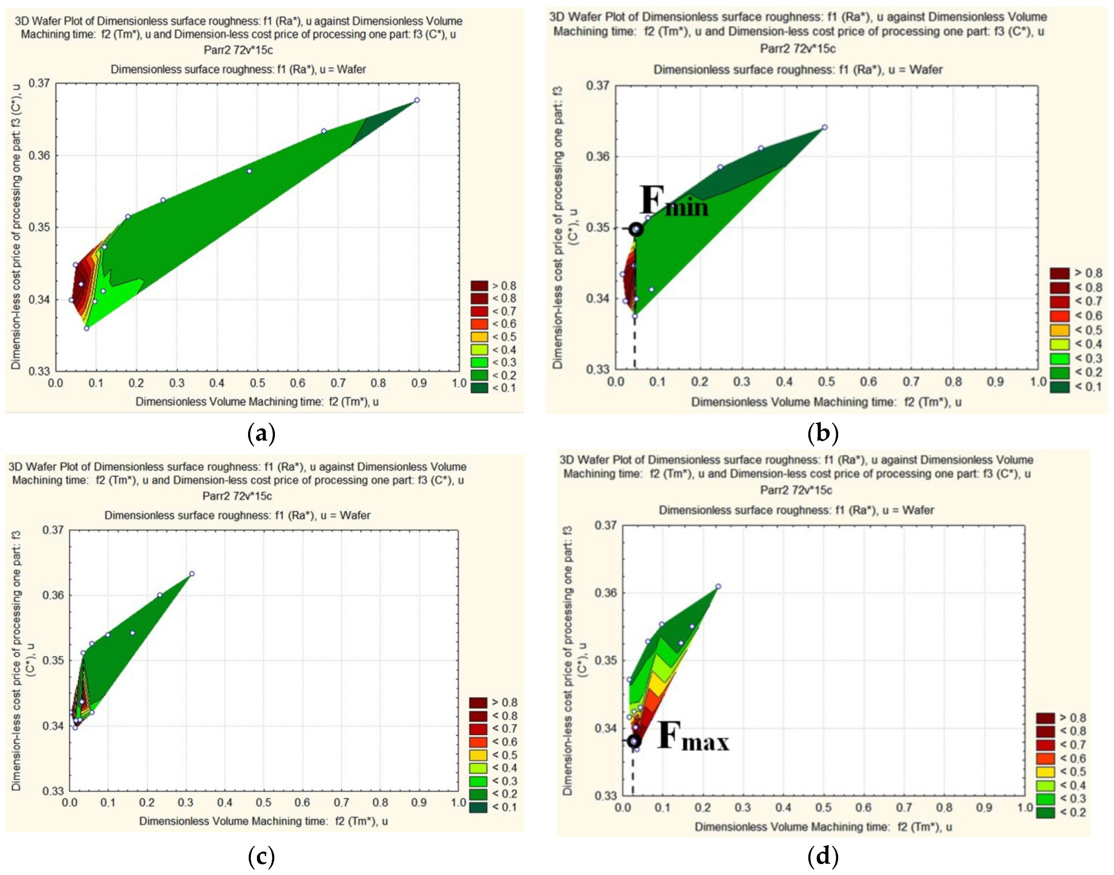
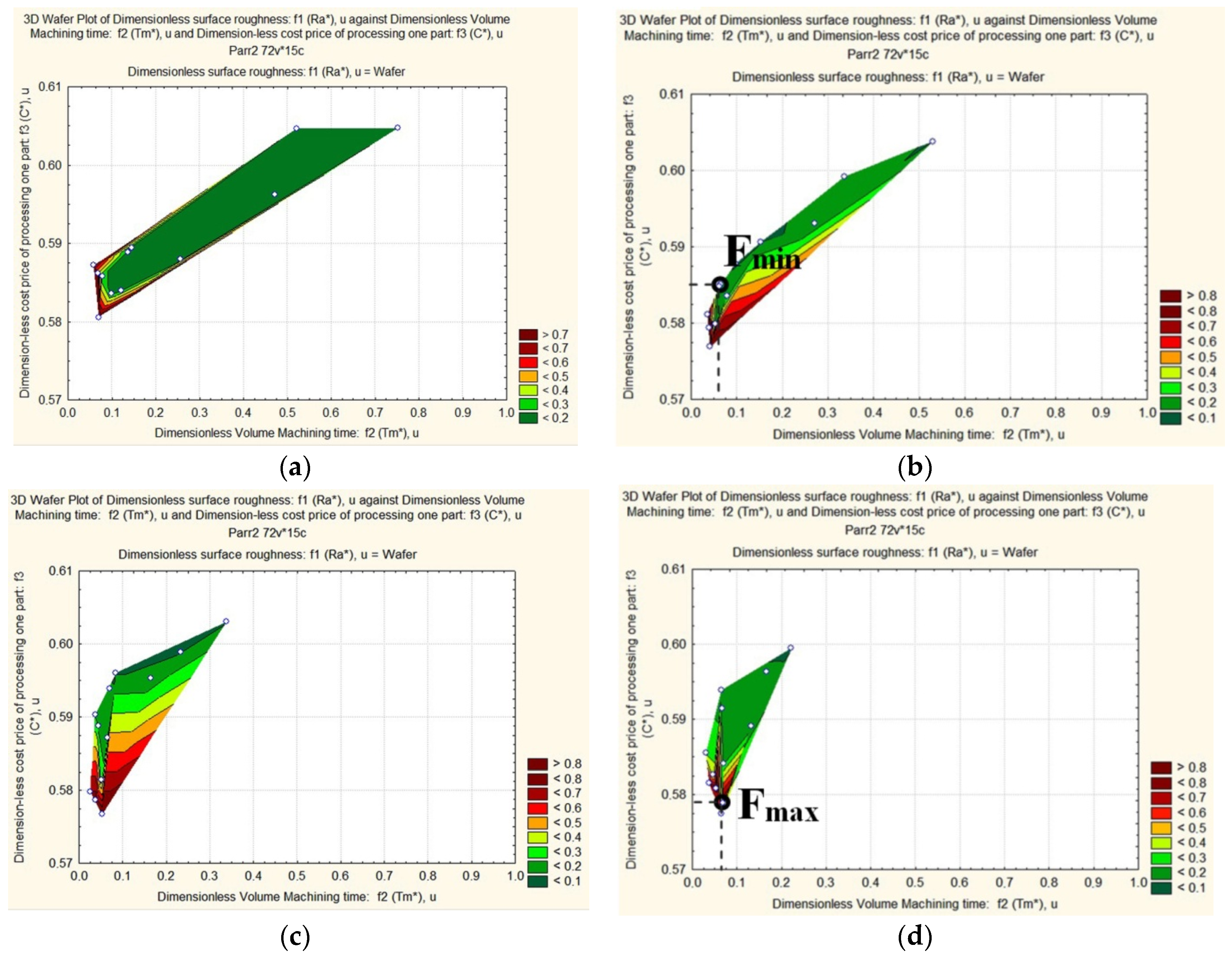
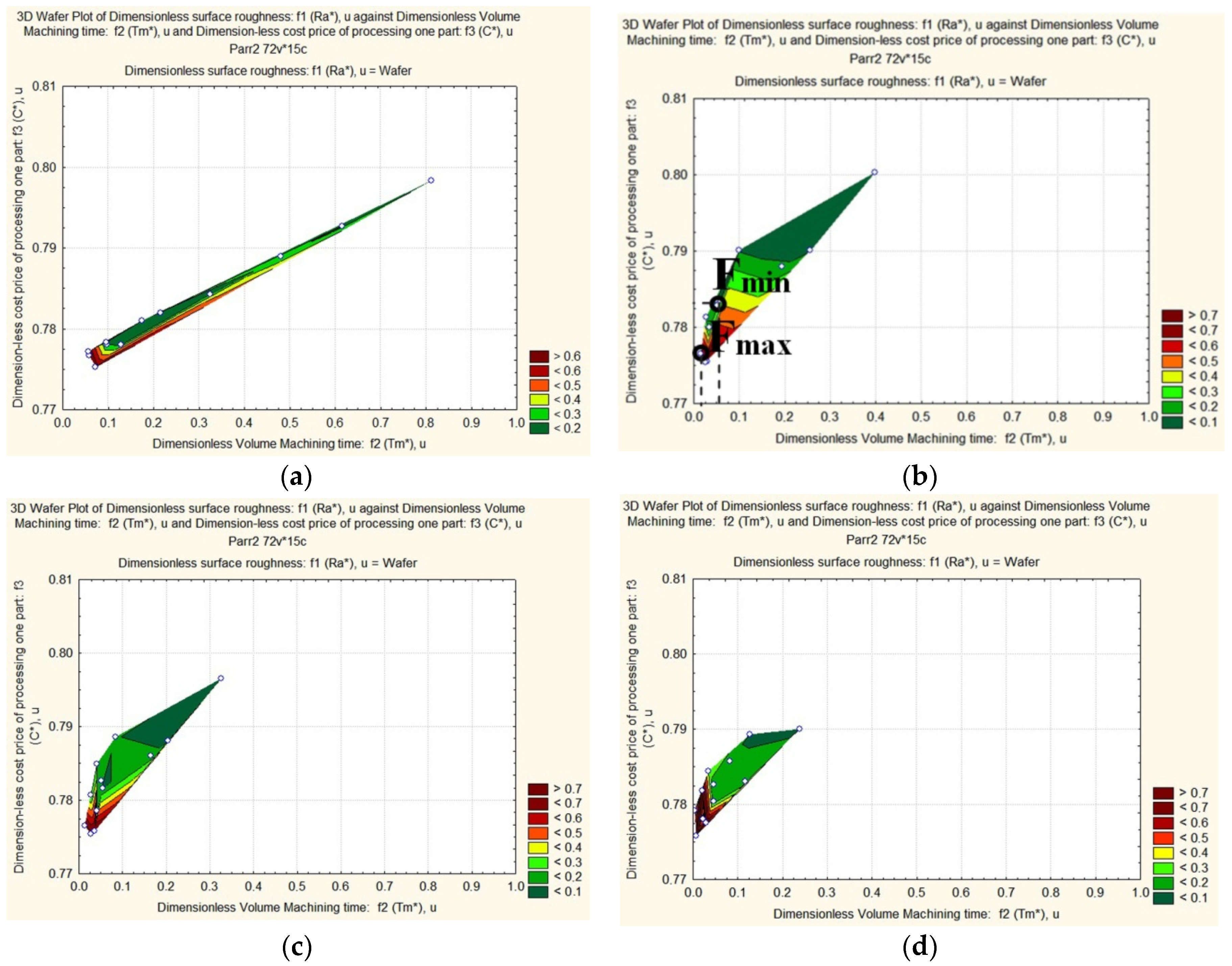
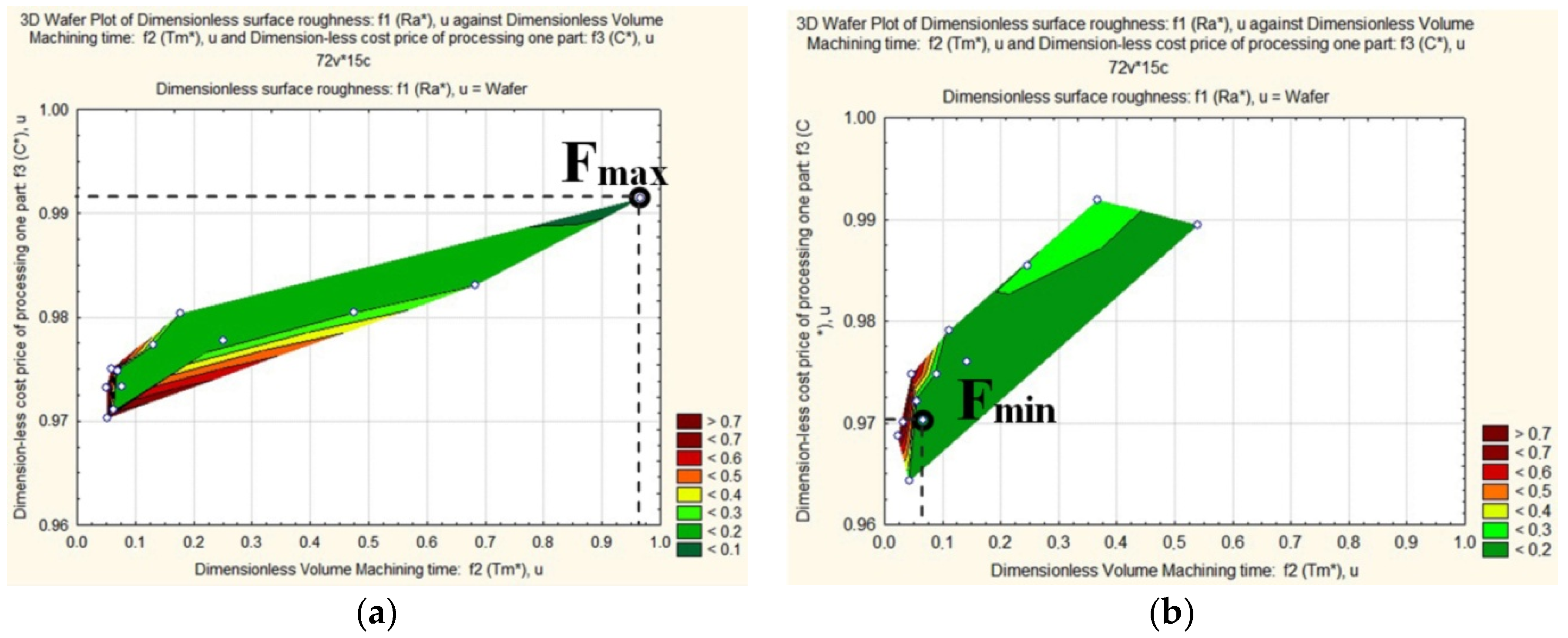
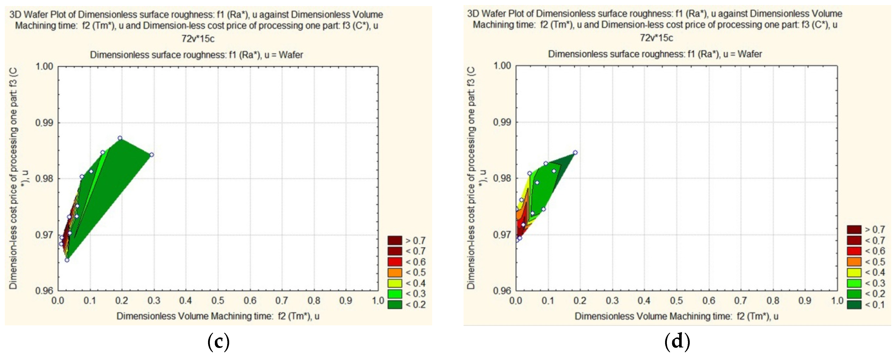
3.5. Establishment of a Pareto Frontier
The target function is represented by a vector length in a normalized space that connects the origin of the coordinates with the point of the three-dimensional surface of estimates. The shortest length at the foot of the apexes, А, of the
Ra* ridge, in the area with the lowest
С* and
Tm* values, have to be defined (see
Figure 7a–d). For this purpose, we shall consider projections of surface estimates at fixed depths of cut:
ap = 0.1 mm,
ap = 0.15 mm,
ap = 0.2 mm,
ap = 0.25 mm,
ap = 0.3 mm,
ap = 0.35 mm, and
ap = 0.4 mm (
Figure 8,
Figure 9,
Figure 10 and
Figure 11).
The above figures (
Figure 8,
Figure 9,
Figure 10 and
Figure 11) depict a decreasing depth of cut from
ap = 0.1 to
ap = 0.4 mm, while the area of the maximum values of dimensionless roughness transforms itself into a decreased projection area due to its shorter ridges. The surface roughness projection area also decreased: in the case of ET-500, the area decreased 1.75-fold (see
Figure 8а–d), in the case of ECAP-2 hardening, the area decreased 1.81-fold (see
Figure 9а–d), in the case of ECAP-4, the area decreased 2.45-fold (see
Figure 10а–d), and in the case of ECAP-6, the area decreased 3.1-fold (see
Figure 11а–d).
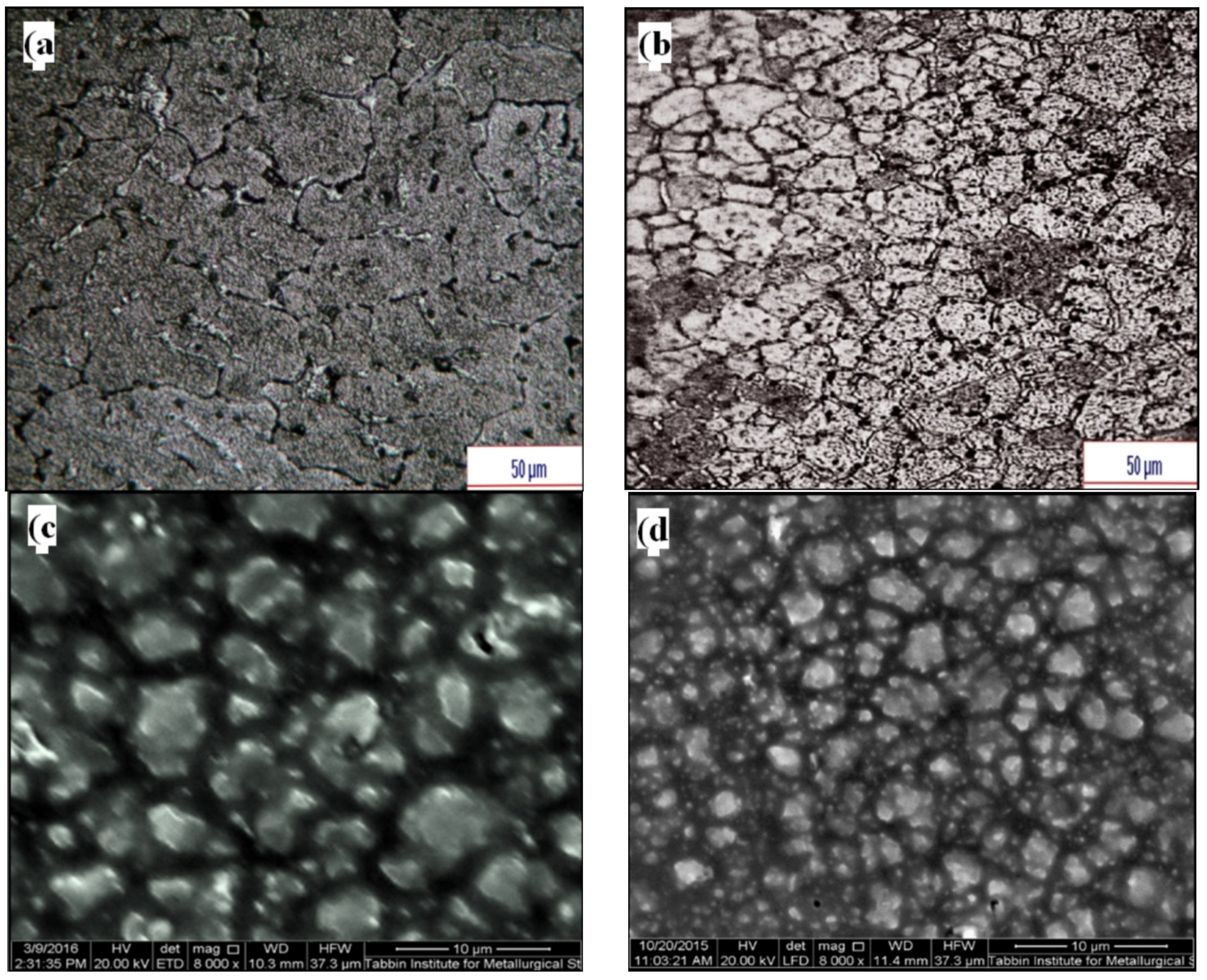
The chip samples extruded at 500 °C had a grain size of 15.9 μm and the effect of 2, 4, and 6 ECAP passes resulted in grain refinement of about 5, 3.28 and 2.46 μm respectively. Grain refinement was accompanied by an increase in microhardness hardness from 41 HV to 110 HV and an increase in the ultimate tensile strength from 132.4 to 403 MPa, as shown in
Table 4. The higher hardness consequently resulted in improved surface finish; due to the hardness of the processed material and low plastic flow capability. A behavior that was attributed to the brittle nature of the interaction between the cutting tool and the workpiece surface, in the same way as in hard materials, which provoked material separation rather than plastic flow that resulted in surface irregularities. Surface roughness was found to increase at increasing feed rates and depths of cut, which resulted in larger cut areas that were consequently associated with higher cutting forces and higher friction. These values, once again, resulted in a poor surface finish. It was noted from the surface roughness profile that high feed rates were associated with higher roughness levels marking horizontal spacing. At higher depth of cuts, the vertical spacing between peaks and valleys of the surface irregularities was also larger. Thus, higher feed rates and depth of cuts led to higher surface roughness (see
Table 5,
Table 6,
Table 7 and
Table 8).
Tm* was the design criterion and its value was only determined by the cutting conditions (vc, ap, fr). It was not dependent on the properties of the machined material (see Formula (1)). Hence, the range of this criterion in no way depended on the hardening method selected for the AA6061 alloy.
Having analyzed the representation of the second criterion C* (see Formula (2)), it was concluded that the major contribution to the cost of machining was due to the AA6061 alloy hardening process. The range of C* values tripled when ECAP-6 was chosen, in which case the maximum strength (microhardness and limit strength) of AA6061 and the minimum surface roughness were obtained.
The optimum has to be located at the foot of the apexes, А, in the area of high-speed turning conditions at which maximum tool wear is possible. According to
Figure 8,
Figure 9,
Figure 10 and
Figure 11, the cutting conditions are limited to a depth of cut of
ap = 0.2 mm (obtaining an AA6061 workpiece with ET-500 extrusion),
f (0.096; 0.050; 0.350; 0.134),
ap = 0.2 mm; (ECAP-2 hardening of an AA6061 alloy workpiece
f (0.112; 0.065; 0.585; 0.462),
ap = 0.25 mm; (ECAP-4 hardening of an AA6061 alloy workpiece,
f (0.083; 0.055; 0.783; 0.582), and
ap = 0.2 mm; and (ECAP-6 hardening of an AA6061 alloy workpiece,
f (0.115; 0.066; 0.970; 0.715), because in this case all the
Ra* values were located near the minimum vector estimation,
f, which are marked by the points
Fmin. The maximum vector estimates,
f, are marked by the
Fmax points.
At these depths of cut and
Fmin, three graphical dependencies,
Ra* =
f(
С*,
Tm*), were constructed. Each one corresponded to the fixed
vc = 100 m/min,
vc = 150 m/min,
vc = 200 m/min and variable
fr. After matching the curves with the projections (see
Figure 8b,
Figure 9b,
Figure 10b and
Figure 11b), we obtained reference points for the Pareto frontier. The following cases are shown in
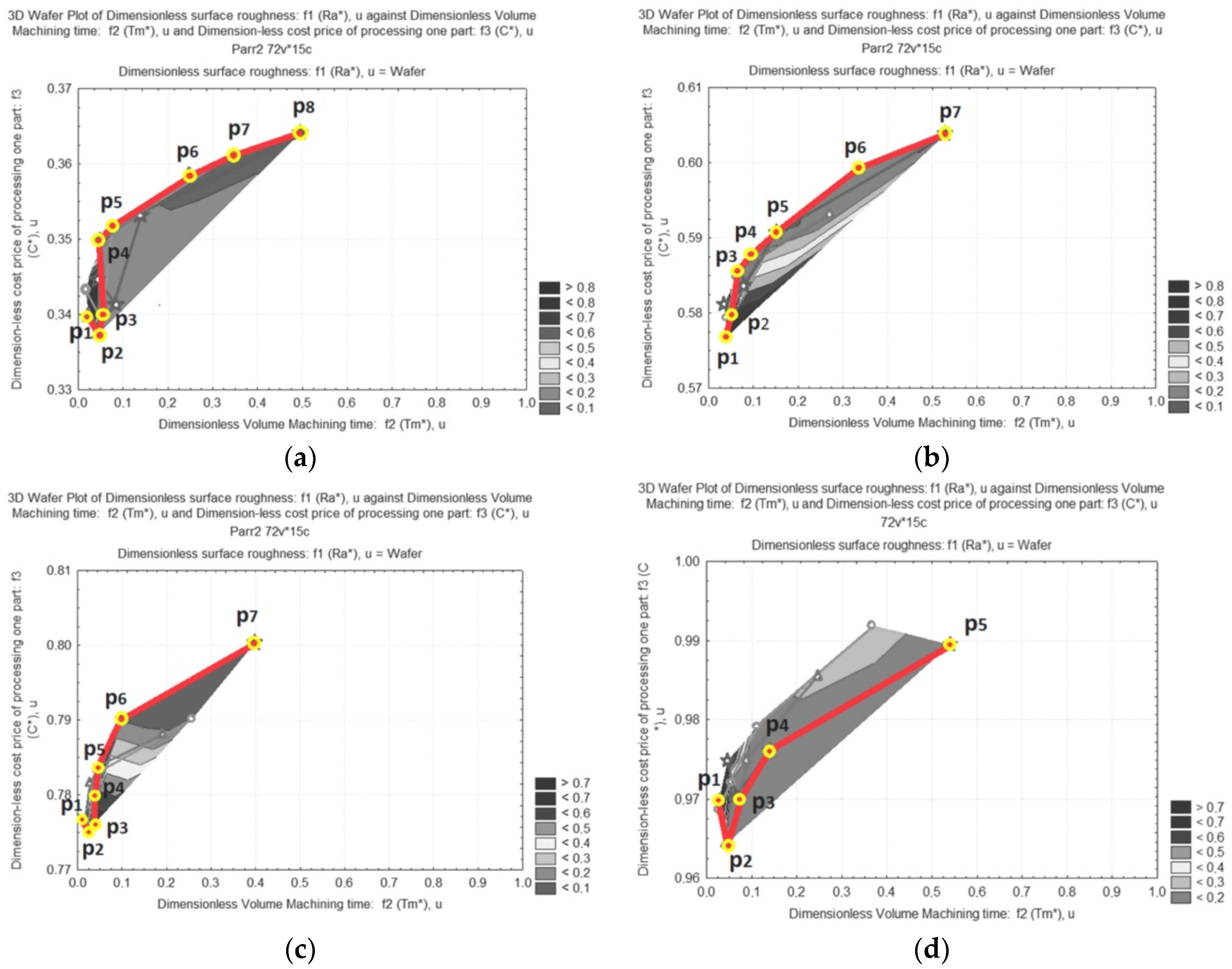
Figure 12a–d: an AA6061 workpiece obtained with ET-500 extrusion р
1 (0.857; 0.024; 0.340); р
2 (0.182; 0.046; 0.337); р
3 (0.157; 0.050; 0.340); р
4 (0.096; 0.050; 0.350); р
5 (0.098; 0.078; 0.351); р
6 (0.075; 0.249; 0.358); р
7 (0.069; 0.345; 0.361); р
8 (0.078; 0.496; 0.364) (see
Figure 12a); ECAP-2 hardening of an AA6061 alloy workpiece р
1 (0.804; 0.042; 0.577); р
2 (0.170; 0.054; 0.580); р
3 (0.112; 0.065; 0.585); р
4 (0.094; 0.098; 0.588); р
5 (0.097; 0.153; 0.591); р
6 (0.107; 0.337; 0.599); р
7 (0.099; 0.530; 0.604) (see
Figure 12b); ECAP-4 hardening of an AA6061 alloy workpiece р
1 (0.767; 0.016; 0.777); р
2 (0.736; 0.026; 0.775); р
3 (0.708; 0.029; 0.776); р
4 (0.147; 0.034; 0.780); р
5 (0.083; 0.055; 0.783); р
6 (0.092; 0.100; 0.790); р
7 (0.091; 0.398; 0.800) (see
Figure 12c) and ECAP-6 hardening of an AA6061 alloy workpiece р
1 (0.758; 0.032; 0.970); р
2 (0.165; 0.043; 0.964); р
3 (0.115; 0.066; 0.970); р
4 (0.104; 0.143; 0.976); р
5 (0.149; 0.539; 0.989) (see
Figure 12d).
The Pareto frontier for the aluminum workpiece obtained with ET-500 extrusion (see
Figure 12a) has the following sections. Section I, between point p
1 and point p
2, corresponds to the following cutting conditions:
vc = 200 m/min,
ap = 0.20 mm,
fr = 0.15…0.081 mm/rev. Section II, between point p
2 and point p
3, corresponds to the following cutting conditions:
vc = 200…150 m/min,
ap = 0.20 mm,
fr = 0.081 mm/rev. Section III, between point p
3 and point p
4, corresponds to the following cutting conditions:
vc = 150…200 m/min,
ap = 0.20 mm,
fr = 0.081…0.045 mm/rev. Section IV, between points p
4 and p
5, corresponds to the following cutting conditions:
vc = 200…150 m/min,
ap = 0.20 mm,
fr = 0.045 mm/rev. Section V, between points p
5 and p
6, corresponds to the following cutting conditions:
vc = 150…200 m/min,
ap = 0.20 mm,
fr = 0.45…0.012 mm/rev. Section VI, between points p
6 and p
7, corresponds to the following cutting conditions:
vc = 200…150 m/min,
ap = 0.20 mm,
fr = 0.012 mm/rev. Section VII, between points p
7 and p
8, corresponds to the following cutting conditions:
vc = 150…100 m/min,
ap = 0.20 mm,
fr = 0.012 mm/rev. p
3 is a special point on the Pareto curve. These points correspond to absolute minimums of the length of vector
f* (Ra* = 0.096 u,
Tm* = 0.050 u,
С* = 0.350 u,
f* = 0.314 u).
The Pareto frontier for the ECAP-2 hardened aluminum workpiece (see
Figure 12b) has the following sections. Section I, between point p
1 and point p
2 corresponds to the following cutting conditions:
vc = 200 m/min,
ap = 0.20 mm,
fr = 0.15…0.081 mm/rev. Section II, between point p
2 and point p
3, corresponds to the following cutting conditions:
vc = 200 m/min,
ap = 0.20 mm,
fr = 0.081…0.045 mm/rev. Section III, between point p
3 and point p
4, corresponds to the following cutting conditions:
vc = 200…150 m/min,
ap = 0.20 mm,
fr = 0.045 mm/rev. Section IV, between points p
4 and p
5, corresponds to the following cutting conditions:
vc = 150…100 m/min,
ap = 0.20 mm,
fr = 0.045 mm/rev. Section V, between points p
5 and p
6, corresponds to the following cutting conditions:
vc = 100…150 m/min,
ap = 0.50 mm,
fr = 0.045…0.012 mm/rev. Section VI, between points p
6 and p
7, corresponds to the following cutting conditions:
vc = 150…100 m/min,
ap = 0.20 mm,
fr = 0.012 mm/rev. p
3 is a special point on the Pareto curve. These points correspond to the absolute minimum of the length of vector
f* (Ra* = 0.112 u,
Tm* = 0.065 u,
С* = 0.585 u,
f* = 0.462 u).
The Pareto frontier for the ECAP-4 hardened aluminum workpiece (see
Figure 12c) has the following sections. Section I, between point p
1 and point p
2, corresponds to the following cutting conditions:
vc = 200…150 m/min,
ap = 0.25 mm,
fr = 0.15 mm/rev. Section II, between point p
2 and point p
3, corresponds to the following cutting conditions:
vc = 150…100 m/min,
ap = 0.25 mm,
fr = 0.15 mm/rev. Section III, between point p
3 and point p
4, corresponds to the following cutting conditions:
vc = 100…150 m/min,
ap = 0.25 mm,
fr = 0.15…0.081 mm/rev. Section IV, between points p
4 and p
5, corresponds to the following cutting conditions:
vc = 150 m/min,
ap = 0.25 mm,
fr = 0.081…0.045 mm/rev. Section V, between points p
5 and p
6, corresponds to the following cutting conditions:
vc = 150…100 m/min,
ap = 0.25 mm,
fr = 0.045 mm/rev. Section VI, between points p
6 and p
7, corresponds to the following cutting conditions:
vc = 100 m/min,
ap = 0.25 mm,
fr = 0.045…0.012 mm/rev. p
1 and p
5 are special points on the Pareto curve. p
1 is the absolute maximum of surface roughness
Ra* (
Ra* = 0.767 u,
Tm* = 0.016 u,
С* = 0.777 u,
f* = 0.818 u). p
5 is the absolute minimum of the length of vector
f* (
Ra* = 0.083 u,
Tm* = 0.055 u,
С* = 0.783 u,
f* = 0.582 u).
The Pareto frontier for the ECAP-6 hardened aluminum workpiece (see
Figure 12d) has the following sections. Section I, between point p
1 and point p
2, corresponds to the following cutting conditions:
vc = 200 m/min,
ap = 0.20 mm,
fr = 0.15…0.081 mm/rev. Section II, between point p
2 and point p
3, corresponds to the following cutting conditions:
vc = 200…100 m/min,
ap = 0.20 mm,
fr = 0.081 mm/rev. Section III, between point p
3 and point p
4, corresponds to the following cutting conditions:
vc = 100 m/min,
ap = 0.20 mm,
fr = 0.081…0.045 mm/rev. Section IV, between points p
4 and p
5, corresponds to the following cutting conditions:
vc = 100 m/min,
ap = 0.20 mm,
fr = 0.045…0.012 mm/rev. p
3 is a special point on the Pareto curve. These points correspond to absolute minimum of the length of vector
f* (
Ra* = 0.115 u,
Tm* = 0.066 u,
С* = 0.970 u,
f* = 0.715 u).
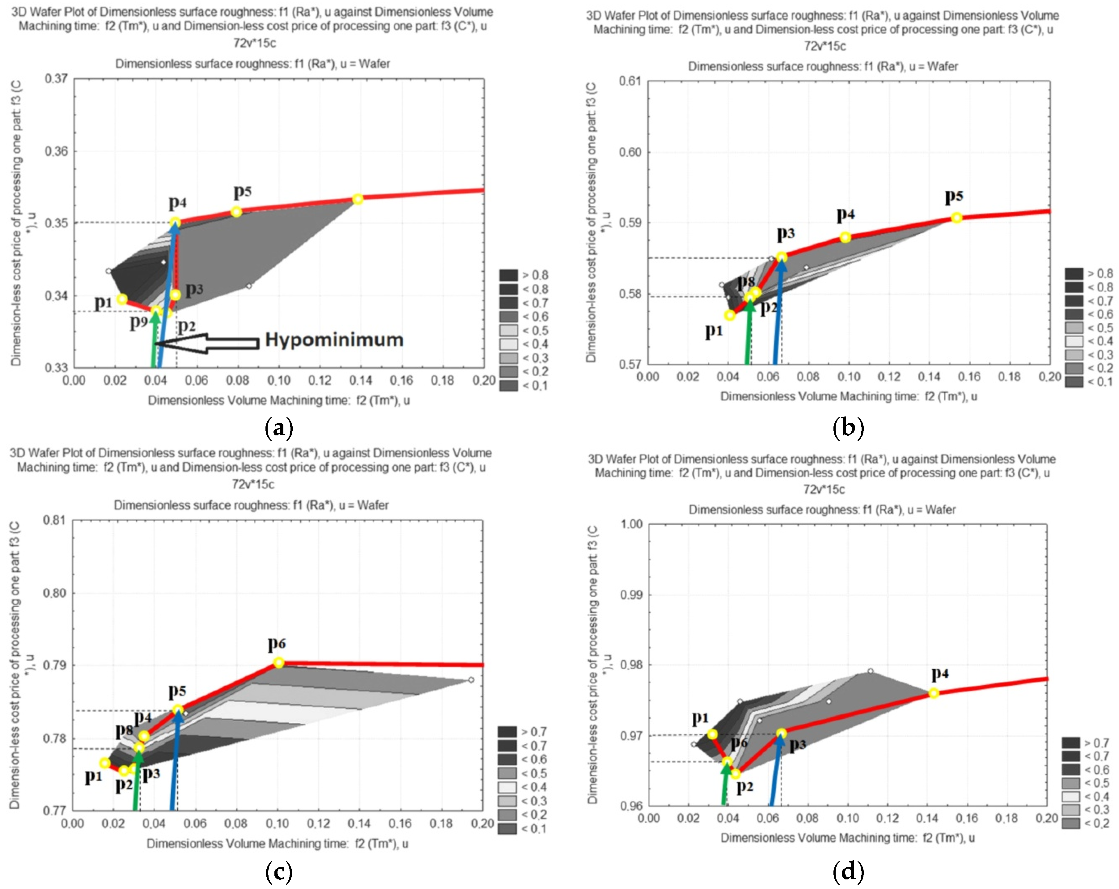
3.6. Establishment of Optimum Turning Conditions
The optimum turning conditions may now be established, which involves narrowing the set of Pareto optimal decisions to a set of Pareto non-dominated decisions. For this purpose, the method of expert assessments was used to establish the lower importance of the dimensionless criterion of surface roughness as compared to the machining time for unit volume removal,
Tm*, and the cost price of processing,
C*. As a result, Pareto non-dominated estimates are presented by the shortest three-dimensional vectors,
f, located above the blue ones and at the angles of 17°, 14°, 8°, and 9° to the plane,
f3f2, for the ET-500 aluminum alloy workpieces, hardened by the ECAP-2, ECAP-4, and ECAP-6 processes, respectively (
Figure 13a–d). The end points of these vectors coincided with point 4 on the Pareto curve for the aluminum workpiece obtained with ET-500 extrusion, with point 3 on the Pareto curve for the ECAP-2 hardened aluminum workpiece, with point 5 on the Pareto curve for the ECAP-4 hardened aluminum workpiece and with point 3 on the Pareto curve for the ECAP-6 hardened aluminum workpiece. They turned out to be the global minima in the case of unconditional optimization with the relation of importance
f1:
f2:
f3 = 1.0:0.5:3.6 (for the aluminum workpiece obtained with ET-500 extrusion),
f1:
f2:
f3 = 1.0:5.2:0.6 (ECAP-2 hardening),
f1:
f2:
f3 = 1.0:9.0:0.6 (ECAP-4 hardening) and
f1:
f2:
f3 = 1.0:8.4:0.6 (ECAP-6 hardening). With the actual coordinates, the global minimum corresponds to
Ra = 0.231 µm,
Tm = 0.416 min/cm
3,
C = 7.223
$),
vc = 200 m/min,
ap = 0.2 mm,
fr = 0.045 mm/rev (the case of obtaining an AA6061 workpiece with ET-500 extrusion),
Ra = 0.269 µm,
Tm = 0.541 min/cm
3,
C = 12/074
$),
vc = 200 m/min,
ap = 0.2 mm,
fr = 0.045 mm/rev (ECAP-2 hardening),
Ra = 0.199 µm,
Tm = 0.458 min/cm
3,
C = 16/161
$),
vc = 150 m/min,
ap = 0.25 mm,
fr = 0.045 mm/rev (ECAP-4 hardening) and
Ra = 0.267 µm,
Tm = 0.549 min/cm
3,
C = 20.020
$),
vc = 100 m/min,
ap = 0.2 mm,
fr = 0.081 mm/rev (ECAP-6 hardening).
After imposing additional restrictions, namely the requirements of the design documentation, the minimum acceptable surface roughness value was established. It corresponded to 0.800 μm or the following points on the Pareto curves: р
9 (0.330; 0.041; 0.337; 0.485) in
Figure 13a), р
8 (0.330; 0.051; 0.579; 0.554) in
Figure 13b, р
8 (0.330; 0.031; 0.778; 0.667) in
Figure 13c, and р
6 (0.330; 0.039; 0.966; 0.785) in
Figure 13d. In this case, the valid relation of importance of the optimization criteria (the green vectors of estimates) become: for the aluminum workpiece obtained with ET-500 extrusion,
Ra*/
Tm*/
С* = 1.0:0.1:2.3, and for points р
4 and р
9, the valid preference was х
9 >
X х
4 and the induced preference was х
9 >
X х
4; for the ECAP-2 hardened aluminum workpiece,
Ra*/
Tm*/
С* = 1.0:0.2:2.3, and for points р
3 and р
8, the valid preference was y
8 >
Y y
3 and the induced preference was х
8 >
X х
3; for the ECAP-4 hardened aluminum workpiece
, Ra*/
Tm*/
С* = 1.0:0.1:2.4, and for points р
8 and р
5, the valid preference was y
8 >
Y y
5 and the induced preference was х
8 >
X х
5; for the ECAP-6 hardened aluminum workpiece,
Ra*/
Tm*/
С* = 1.0:0.1:2.9, and for points р
3 and р
6, the valid preference was y
6 >
Y y
3 and the induced preference was х
6 >
X х
3.
As a result, the set of selected estimates Sel Y was limited to the green vectors, and the set of selected decisions, Sel X, to the three-dimensional vectors of the optimum cutting parameters for the workpiece obtained with ET-500 extrusion: vc = 200 m/min, ap = 0.2 mm, fr = 0.103 mm/min, for the ECAP-2 hardened workpiece: vc = 200 m/min, ap = 0.2 mm, fr = 0.101 mm/min, for the ECAP-4 hardened workpiece: vc = 143 m/min, ap = 0.25 mm, fr = 0.104 mm/min; for the ECAP-6 hardened workpiece: vc = 200 m/min, ap = 0.2 mm, fr = 0.105 mm/min.
In summary, it should be noted that the hypolocal optimum corresponded to the green vector estimates for the workpiece obtained with ET-500 extrusion without hardening (see
Figure 13a).

 ,
, 


