Article

A New Approach to Simulate HSLA Steel Multipass Welding through Distributed Point Heat Sources Model

by
Dario Magno Batista Ferreira
1,
Antonio do Nascimento Silva Alves
2,
Rubelmar Maia de Azevedo Cruz Neto
2,
Thiago Ferreira Martins
2 and
Sérgio Duarte Brandi
2,*
1
Mechanical Engineering Coordination, Instituto Federal do Espírito Santo—Ifes, Vitória 29040-780, Brazil
2
Metallurgical and Materials Engineering Department, Universidade de São Paulo—USP, São Paulo 05508-030, Brazil
*
Author to whom correspondence should be addressed.
Metals 2018, 8(11), 951; https://doi.org/10.3390/met8110951
Submission received: 28 August 2018 / Revised: 17 September 2018 / Accepted: 18 September 2018 / Published: 15 November 2018
(This article belongs to the Special Issue Science, Characterization and Technology of Joining and Welding)

Abstract

:
Mechanical properties of welded joints depend on the way heat flows through the welding passes. In multipass welding the reheating of the heat affected zone (HAZ) can form local brittle zones that need to be delimited for evaluation. The difficulty lies in the choice of a model that can simulate multipass welding. This study evaluated Rosenthal’s Medium Thick Plate (MTP) and the Distributed heat Sources (DHS) of Mhyr and Gröng models. Two assumptions were considered for both models: constant and temperature-dependent physical properties. It was carried out on a multipass welding of an API 5L X80 tube, with 1016 mm (42″) external diameter, 16 mm thick and half V-groove bevel, in the 3G up position. The root pass was welded with Gas Metal Arc Welding (GMAW) process with controlled short-circuit transfer. The Flux Cored Arc Welding (FCAW) process was used in the filling and finishing passes, using filler metal E111T1-K3M-JH4. The evaluation criteria used were overlapping the simulated isotherms on the marks revealed in the macrographs and the comparison between the experimental thermal cycle and those simulated by the proposed models. The DHS model with the temperature-dependent properties presented the best results and simulated with accuracy the HAZ of root and second welding passes. In this way, it was possible to delimit the HAZ heated sub-regions.

1. Introduction

In electric arc welding, the addition and the base metals are fused by the heat source and it still imposes phase changes in the solid base metal (BM), i.e., in the heat affected zone (HAZ) [1]. The retention time above certain temperatures reached along the HAZ dissolves precipitates and promotes its redistribution in the austenitic matrix together with grain growth [2,3,4]. Further, the energy retention times above certain temperatures, the peak temperatures and cooling rates are different along the HAZ. Hence, different microstructural regions throughout the HAZ width are created, so that its final microstructures differ significantly from that of the original BM [5,6]. Figure 1 presents the microstructures in the experimental HAZ regions of an API 5L X80 steel, in which it is possible to observe different grain sizes and microstructures. The coarse-grained HAZ (CGHAZ) region presents grains whose diameter is greater than the others. Its microstructure is composed by ferrite with a second phase of carbides, while the others are composed by ferrite with aggregate ferrite-carbide. The intercritical HAZ (ICHAZ) grains still present some orientation from the base metal grains. Therefore, the HAZ physical properties also differ from that of BM. The hardness and toughness are mechanical properties that are dependent of the welding thermal cycle and they are reference parameters for measuring the steel’s weldability [7].
The study and domain of these transformations are required for the prediction and control of the resulting microstructure and welded-joint required properties, consequently [6,7]. Figure 2 shows schematically the HAZ sub-regions in a high-strength low-alloy steel (HSLA) multipass welding, HT50 [5].
The HAZ root pass, represented by Figure 2a, is characterized by different microstructural regions: CGHAZ, fine-grained HAZ (FGHAZ), ICHAZ and subcritical HAZ (SCHAZ). Figure 2b presents the second welding pass that promotes the formation of a new HAZ adjacent to its corresponding pass with the same microstructural regions shown before. However, this second welding pass partially affects the previous HAZ, so that new microstructure sub-regions arise. Traveling on the root CGHAZ from the top towards to the schematic bottom face specimen, it is possible to recognize that a sub-region was reheated above the recrystallization temperature. It is named CG-CGHAZ. The next lower portion thereof CGHAZ is reheated in the temperature range in which there is grain refinement—the RG-CGHAZ. The same CGHAZ is still reheated within the range of intercritical temperature, making arise the IR-CGHAZ. This subregion needs more attention to be known as the local brittle zone [5,8] (LBZ). The temperature range between Ac1 and Ac3, is favorable to MA microconstituent formation in multipass weldments [2,5,8], as it can deteriorate the steel toughness, depending on its size and distribution in the ferritic matrix [9,10]. The following sub-region is reheated in the subcritical temperature range: it arises the SC-CGHAZ. For the last, remains the unaffected root CGHAZ. Similarly, the third welding pass, shown in Figure 2c, affects the previous HAZ and the root pass HAZ, but is less intense than the second one.
Software packages that use the Finite Element Method (FEM) have been used successfully to simulate welding, in which the material physical properties are temperature dependent [11], to calculate isotherms, thermal cycles, residual stresses [12,13], distortions [14] and uses a volumetric heat source with a Gaussian power distribution. The heat source dimensions are adjusted by weld bead macrography [15,16,17]. FEM has also been used to simulate multipass welding to solve these same questions, however, the previous HAZ reheating through subsequent welding pass is not evaluated [18,19,20,21,22]. Single pass welding simulation is a costly operation for the FEM, the more expensive it will be for multipass welding simulation [18,23]. HAZ simulation in the weld cross section through FEM presents the difficulty of the delimitation of the isotherms maximum widths that are in different planes for different values of thickness. HAZ reheating simulation is another difficulty presented for FEM software packages because the user does not have flexibility to save the isotherms coordinates of each weld pass.
Due to the presented difficulties, analytical solutions for the heat flux in the welding will be presented.
The analytical solutions developed by Rosenthal [24] to describe the welding heat flow considered the quasi-stationary heat flow regime in an autogenous welding. The analytical solutions or Rosenthal’s model is based on the Fourier differential equation, described by Equation (1). In this equation, λ is thermal conductivity and ρ c p is the volumetric thermal capacity and Q0 is a component of energy generation.
x ( λ T x ) + y ( λ T y ) + z ( λ T z ) + Q 0 = ρ c p T t
The heat transfer models developed by Rosenthal [24,25,26], called thin plate (2D) model and thick plate (3D) model are most widely used for their simplicity, in order to analyze heat flow within a welded joint. Later, Jhaveri et al. [27] proposed a dimensionless parameter, called relative thickness ( τ ), which defines the relative thickness interval to use on 2D or 3D heat transfer model. Therefore, the thin plate heat transfer model should be used when the value of τ is less than 0.6. On the other hand, when the value of τ is more than 0.9 the thick plate solution is employed. There is a gap among 0.6–0.9 relative thickness, in which both models (2D and 3D) are not applied. The medium thick plate (MTP) is another model developed by Rosenthal [24,26] that can be used in this τ interval, in which the other two models do not present good results [2].
Among the mentioned heat flow models, the MTP model is more robust as it can predict temperature isotherms for thick plate (3D) and for thin plate (2D) heat flows [2]. To find the solution of medium thick plate model, some hypotheses were assumed [24]:
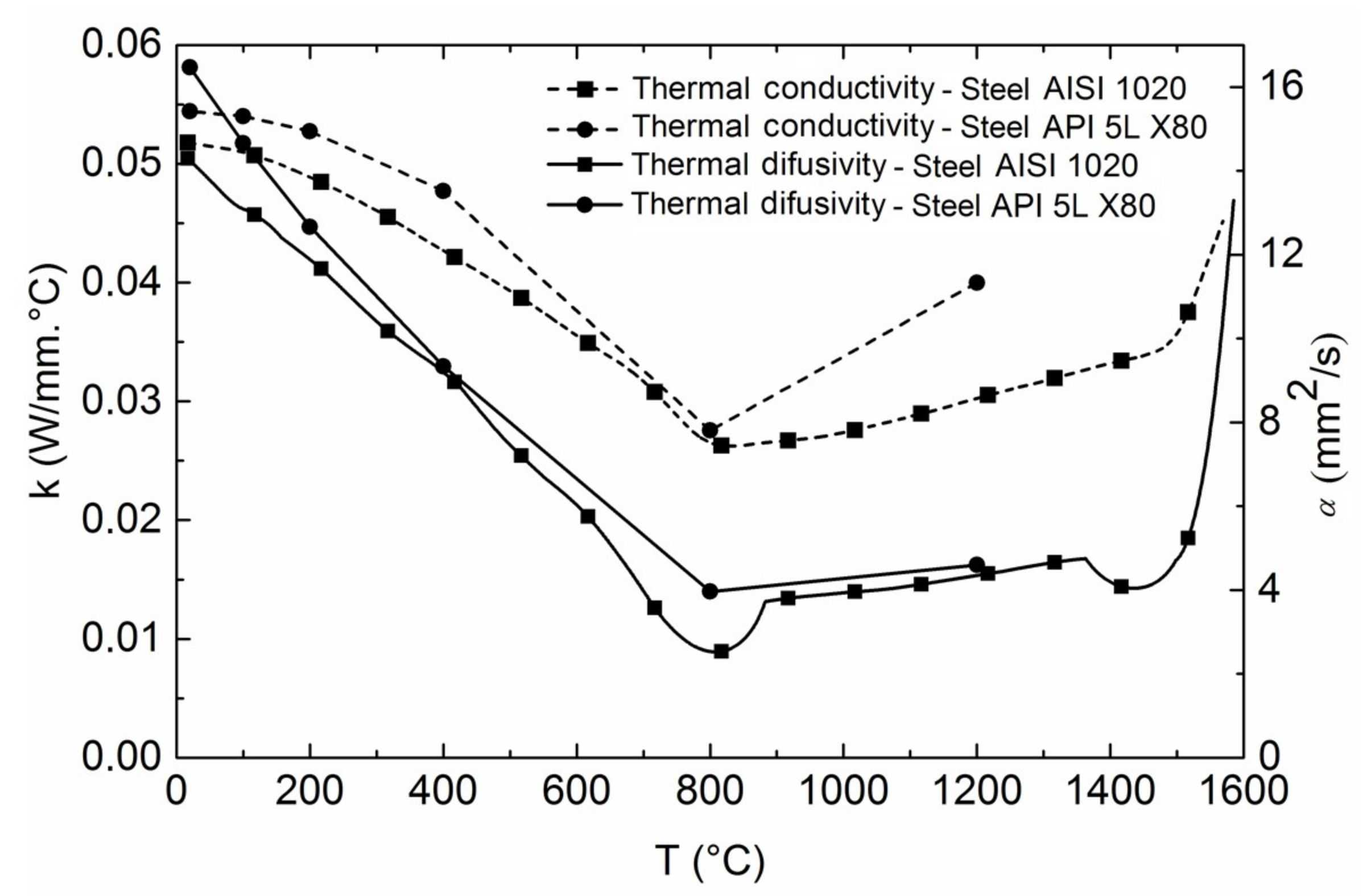
  • Physical properties constant at room temperature (λ and α), independent of temperature;
  • Point heat source moves in a straight line with constant speed ν;
  • No energy generated or consumed within the plate, i.e., Q0 = 0;
  • All the heat flow is transmitted by conduction. Radiation and convection through surfaces are neglected;
  • The plate is semi-infinite, with a thickness d;
  • The initial condition is defined by Equation (2).
    T ( 0 ) = T 0
  • The boundary conditions are defined by Equation (3);
    { T z = 0 ,   z = 0 T z = 0 ,   z = d
The simplification imposed by Equation (3) implies that there is no heat loss by radiation and convection through the upper and lower plate surfaces, i.e., both surfaces are adiabatic. This condition is achieved by the method of images, which considers specular reflections of the actual source by imaginary ones (…, 2q−2, 2q−1, 2q1, 2q2, …), in relation to the planes z = 0 and z = d, as shown in Figure 3.
The coordinate system used to solve Equation (1) defines that the x-axis is related to the welding direction and the weld pool length. The y-axis is related to the width of HAZ and weld pool, while the z-axis is related to the plate thickness and the weld pool depth. The contribution from these heat sources allows to obtain the temperature distribution solution, in the form of a convergent series, according to Equation (4a).
T T 0 = q 0 2 π λ e x p ( v x 2 α ) [ i = i = + e x p ( v 2 α R i ) ]
where
R i = x 2 + y 2 + ( z 2 i d ) 2
Equation (4a,b) define the solution of Equation (1) with its initial and boundary conditions in quasi stationary regime, where Ri is the radius vector which measures the distance between the imaginary source qi and the point P where it is intended to calculate its peak temperature. The real heat source is presented by q0 at the origin of the coordinate system, α is the thermal diffusivity, (x, y, z) are the coordinates of the point P and ν is the weld speed.
Figure 4 shows the temperature isosurfaces of 1520 °C, 1000 °C, 700 °C and 500 °C simulating the welding of a low alloy steel with the MTP model, heat input of 1.2 kJ/mm and 14.5 mm of thickness. The shape of the isotherm of 1520 °C indicates a 3D heat flow, while the shape of the isotherm of 500 °C indicates a heat flow between 3D and 2D, because it touches both plate surfaces.
However, a new proposal for the study of welding heat flux was based on the analytical model called discretely distributed point heat sources model (DHS) developed by Myhr and Grong [2], initially intended to predict the convection effects within the weld pool. These effects cause changes in the bead format, called finger, as shown in Figure 5.
The DHS model is based on the point heat sources distribution of Rosenthal′s MTP on a fusion zone cross section, so that the increase in temperature at point P located within the plate is calculated based on the method of images [2], as defined schematically in Figure 6.
The plate surfaces are adiabatic like they are in the MTP model [2,24]. The point heat sources, in this case, are subdivided into ones that are located on the plate (qa) along the y-axis and those immersed in the molten pool (qb) along the z-axis, as shown in Figure 7.
Finally, the temperature at a point is the sum of the power contributions of all point heat sources, as presented in Equation (5).
T T 0 = i [ T ( q a i ) + T ( q b i ) ]
The heat source total power (q0) is the sum of the contributions of all point heat sources, considering the welding arc efficiency (η), arc voltage (V) and welding current (I), as presented by Equation (6).
q 0 = i [ q a i + q b i ] = η V I  
This model, however, was modified by Ramirez and Brandi [28], so that sources q a i located on the y-axis could be displaced from a value Δz into the weld pool, in the z direction. Thus, the point sources could be located on the y-axis, or below it, located anywhere in the y-z plane, since confined inside the weld pool [28]. This model was developed due to the need to simulate multipass welding [28]. The authors considered physical properties independent of temperature and they still used Gleeble® system equipment (Dynamic Systems Inc., Poestenkill, NY, USA) to simulate physically the HAZ. According to the authors, the results were quite satisfactory when compared with experimental and physically simulated data.
Models presented evolution as the boundary conditions imposed on the differential equation and the size of the heat source are close to actual welding situations. The difficulty of applying these models lies in the definition of the values of the physical properties, since they are temperature-dependent. In this way, errors can be made when trying to delimit the HAZ regions, or to simulate thermal cycles with different maximum temperatures.
Thus, this work proposes to evaluate the effectiveness of MTP and DHS models by overlapping the simulated isotherms on the marks revealed in the macrographs and by means of experimental thermal cycle. For both models, the hypothesis of constant and temperature-dependent physical properties will be considered. The best option will be used to simulate the HAZ of multipass welding.

2. Materials and Methods

A girth welding was carried out between two API 5L X80 steel pipe with 1016 mm (42″) diameter and 16 mm wall thickness, whose chemical composition is shown in Table 1.
The joint was manually welded using only half perimeter of the pipes. The root pass was welded by Gas Metal Arc Welding (GMAW) using Surface Tension Transfer Mode (STT®, The Lincoln Electric Company, Cleveland, OH, USA) throughout the mentioned pipe extension. Subsequent passes were welded by the Flux Cored Arc Welding (FCAW) process. The beginning of each weld pass has been displaced to maintain an extension of the previous one free of microstructural changes due to the subsequent beads, as shown in Figure 8.
According to the schematic view of the welded joint, depicted in Figure 8 (Det. A), thermocouple K-type 0.25 mm diameter was welded on the inner pipe surface and in the beginning of welding finishing pass section, at 7.15 mm from the weld centerline. Thus, it was possible to record the thermal cycle during all welding passes from a data acquisition system. K-type thermocouple has a measuring range of −220–1260 °C with an error of ±4.4 °C [29]. Welding parameters were also recorded, as voltage (V) and current (I), in function of time, in the range of 0.0002 s. The average source power was calculated from the instantaneous power values.

Extended Myhr and Grong′s Model

The DHS model was evaluated in this work with some additional considerations to better represent the fusion zone contour, the HAZ isotherms and the thermal cycle, starting with the model proposed by Ramirez and Brandi [28]. That is, since the sources q a i have been displaced from z axis into the weld pool, they will have the same nature as the sources q b j . Therefore, both kind of heat sources will be treated just as qi, and their displacements will assume values of their own coordinates related to system origin, (yqi, zqi). The quasi-stationary heat flow regime, in this case, is represented by Equation (7).
T ( q i ) = q i 4 π λ e ν x 2 α [ m = m = R m υ 2 α R m + n = n = R n υ 2 α R n ]
where,
R m = x 2 + ( y q i y p ) 2 + ( z q i 2 m d z p ) 2  
R n = x 2 + ( y q i y p ) 2 + ( z q i 2 n d + z p ) 2  
Thus, the point heat sources positions and their respective power values became more flexible and η is assumed as a constant value for all of them, which is different from the previous works [2,16,17,28]. However, there is still a question regarding the values to be attributed to the physical properties, as they are dependent on the temperature. Rosenthal, although he formulated the MTP model considering such properties independent of temperature, suggests that they are adjusted step by step [24]. This approach was partially adopted by Azar et al. [16], when using the DHS to simulate the fusion zone isotherm and other two HAZ isotherms in a hyperbaric welding. In their simulation, the physical properties changed by temperature ranges, whose base metal was an API 5L X70 steel.
Starting from the principle that the HAZ has different microstructures, which had undergone different thermal histories along HAZ width, then, it is possible to obtain some inaccuracies when using physical properties by temperature ranges. For this reason, this work proposes to adopt the values of physical properties varying with each simulated isotherm temperature, as well as with simulated thermal cycles. This work still proposes to utilize point heat sources positions and their respective power values to adjust the melting temperature isotherm through the fusion zone contour on the macrograph. Once the heat sources distributions are adjusted, this will be kept simulating other HAZ isotherms and thermal cycles.
The thermal cycle at the P-point within the HAZ was simulated with discretized temperatures by variation of 1 °C from the preheat temperature T0. That is, during the heating stage, the evolution of the temperature versus time was defined by an increase of 1 °C, in relation to the previous temperature (Ti−1) until it reaches a maximum value. The instant ti at which the temperature at the P-point is increased by 1 °C is calculated by Equation (8).
T 1 = T 0
T i = T i 1 + 1 ,   i > 1
t 1 = t ( T 1 ) = 0
t i = t i 1 + Δ t 1 + Δ t 2 2 ,   i > 1
The values of the time intervals Δ t 1 and Δ t 2 were defined as the time required to vary from 1 °C between the temperatures Ti−1 and Ti. For the calculation of Δ t 1 , the physical properties were considered constant and calculated at the temperature Ti−1. An analytical thermal cycle was then calculated from these physical property values and other variables defined in Equation (7). The calculation of Δ t 1 was determined from reading in the thermal cycle, when the temperatures ranged from Ti−1Ti in the P-point.
The value of the time interval Δt2 was calculated using the same methodology, but with the physical properties calculated at temperature Ti. This calculation scheme is shown in Figure 9, which depicts part of the analytical thermal cycles during heating at temperatures (T) and (T + 1), using the physical properties depending on the respective temperatures. The Δtmean was calculated by the arithmetic mean of Δ t 1 and Δ t 2 .
For each value of Ti, the values of the thermal properties, the respective analytical thermal cycle and its maximum temperature— T max ( λ ( T i ) ) —are calculated. The maximum temperature of the discretized heat cycle— T max ( T i ) —is calculated according to Equation (9).
T max ( T i ) = T max ( λ ( T i ) )   i f   | T i T max ( λ ( T i ) ) | 2   ° C
The difference of 2 °C between Ti and T max ( λ ( T i ) ) was chosen to calculate T max ( T i ) because the temperature Ti is increased by 1 °C in the discretized thermal cycle. This value was enough to ensure the convergence criterion.
The cooling stage of the thermal cycle started from the last temperature reached in the heating step and the calculations of Δt1 and Δt2, following the same criterion. However, the next temperature value will decrease by 1 °C with respect to the latest one. Finally, the cooling time interval from 800 °C–500 °C (Δt8−5) was obtained from the final numerically simulated thermal cycle at the interest point.
For the simulation purpose of the HAZ isotherms and thermal cycles, as suggested, the thermal conductivity and diffusivity properties of AISI 1020 steel, as a function of temperature, were used, according to Figure 10.
In this picture, one can notice that the values of AISI 1020 thermal conductivity and thermal diffusivity are close enough to the API 5L X80 steel. The AISI 1020 steel physical properties were used to simulate the welding heat flow for the API 5L X80 steel pipe joint, as these can be estimated from the liquidus temperature to the room temperature.

3. Results

3.1. Comparison between Different Analytical Models

Conventionally, the analytical solutions for welding simulations consider the physical properties as constant, i.e., independent of temperature, just as they were developed [2,24,26,30]. However, in engineering materials, the physical properties are temperature-dependent, such as those shown in Figure 10. To evaluate the DHS proposed model, a comparative study will be carried out with MTP model, initially considering the temperature-independent physical properties and later with the temperature-dependent ones, through the methodology suggested in this work. The welding parameters were the same for all simulations, i.e., the heat source power was equal to 2376 W and the welding speed equal to 1.05 mm/s, that resulted in a heat input of 2.26 kJ/mm. Considering the case in which the physical properties were assumed constant, they were selected at the temperature of 25 °C, in which values were obtained from Figure 10: λ was equal to 0.052 W/mm °C and α equal to 14,208 mm2/s.
The simulation codes were developed through Wolfram Mathematica® software (Version 10.2.0.0 Student Edition, Wolfram Research, Champaign, IL, USA) to determine the isotherms profiles and thermal cycles, using the resource of finding roots, like Newton-Raphson and bisection methods, because the temperature field equations presented before are transcendental functions.
Figure 11 and Figure 12 present the results of simulation in which the physical properties were constants and based on MTP and DHS models, respectively.
In Figure 11, the contours of the original bevel and the weld centerline are highlighted, the point heat source is presented through the white point on the specimen’s bottom surface. The simulated HAZ isotherms are superimposed on the multipass welded joint macrograph to assess the fit between simulated and experimental results. The isotherms of 1520 °C, 1200 °C, 903 °C and 713 °C represent respectively the base metal solidus, recrystallization, Ac3 and Ac1 temperatures. The first one was obtained through Thermo-Calc® software (Version 2.2.1.1, Foundation for Computational Thermodynamics, Stockholm, Sweden), the second value was based on Pickering [31] and the last two of them were determined using dilatomety analysis.
Figure 12 presents the DHS simulation using 19-point heat sources distributed within the melt zone, each one using 8 imaginary sources. Typically, the simulations by DHS use less point heat sources [2,16,17,28]. The greater the amount of point heat sources used in a simulation, the easier to adjust their position and respective power source values. The innermost heat sources are those with the highest power values. The final adjustment of the simulated fusion isotherm to the weld pool cross section is promoted by the most external heat sources, which have the lowest power values. This power distribution of heat sources suggests a Gaussian distribution, as proposed in numerical methods [32,33].
A better fit can be observed between the melt temperature isotherm with the molten zone contour. However, for the other isotherms the fit was worse, i.e., their positions did not coincide with the contours revealed in the macrograph. Table 2 shows the relative error between the positions of 1520 °C and 903 °C simulated isotherms with respect to three reference points located at 1.5 mm, 3.0 mm and 4.5 mm, respectively, above the specimen lower surface.
The following isotherm simulations were carried out with the temperature-dependent physical properties, in which each property value was selected based on the current isotherm temperature value. Figure 13 and Figure 14 present the results considering MTP and DHS models, respectively. It can be observed in Figure 13 that the isotherm’s positions provided a better adjustment in relation to the macrograph revealed contours when compared to the results presented in Figure 11.
Figure 14—which represents the proposed model in this work—shows the DHS simulation using 19-point heat sources distributed within the melt zone, whose power and position distributions were adjusted to simulate molten zone contour. Once the necessary adjustment was done, this configuration remained the same to simulate the other isotherms. The power value of 2376 W used to simulate the 1520 °C isotherm was within the calculated average source power of 1877 ± 920 W. This high standard deviation value was related to the welding process used, which, in this case, was a curt circuit one, in which there is a great current variation. This behavior of the power values is also reported by Azar [16] that calculates the average power from its instantaneous values.
As can be seen, the adjustment of the isotherms on the contour revealed in the macrographs is more accurate in Figure 14 than in Figure 13. Table 3 presents the relative error for both simulations, in the same positions of the reference used before. Negative error values indicate the isotherm position was on the left side of the revealed macrograph contours.
The performance of models was also compared with respect to the simulated thermal cycles. For the cases in which the properties were considered temperature-dependent, the methodology proposed in topic 3 was adopted for both MTP and DHS models. The results of the simulations are summarized in Figure 15 that presents thermal cycles simulated through the same criteria used before in the isotherm profiles determination.
Table 4 presents a thermal cycle performance study based on the maximum temperature (Tmax) reached by a thermocouple and its Δ t 8 5 . The thermal cycles whose physical properties are temperature independent are presented by λ(25 °C) and those whose physical properties are temperature dependent are presented by λ(T). The position used to simulate them was the same where the thermocouple was installed, i.e., 7.15 mm right of the weld center line or 2.35 mm from the molten zone, in which Tmax = 1004.34 °C and Δ t 8 5 = 47.98   s .
It can be seen that the DHS proposed model presented the best answer in relation to Tmax, but not in relation to Δ t 8 5 , whose calculated value was higher than the experimental one. It means that the effect of neglecting heat losses has a small but consistent effect on simulation of the maximum temperature, and probably also has a consistent effect on the time lag difference shown in Figure 15 for thermal cycling.
Another criterion for the thermal cycle evaluation through the proposed DHS model was the Δ t 8 5 variation depending on the maximum temperature reached on the HAZ width. In this case, the z coordinate was set at 1.2 mm above the specimen’s bottom face on the right side of the groove and the results are shown in Figure 16.
In the neighborhood of the molten zone, in the 1489 °C maximum temperature position, the Δ t 8 5 value was 49.5 s. At the lower temperature HAZ end, in the 814 °C maximum temperature position, the Δ t 8 5 value was 54.6 s in the simulated thermal cycle. That is, there was a variation of only 10.3% compared to the minimum Δ t 8 5 value for a variation of 83% in temperature values throughout the HAZ width. This behavior is typical of values found in analytical solutions [2,4,24,27]. In other words, in the weld centerline on the plate upper surface and behind the weld pool, the value of Δ t 8 5 is constant because the coordinate values y and z are null [4,24,34]. However, when these coordinates are inside the HAZ, the Δ t 8 5 variation is very small [4,27,35]. Therefore, a Δ t 8 5 value measured by a thermocouple may be used in whole HAZ extent, whose error is not greater than 10%.

3.2. Multipass Welding Simulation through DHS Model

Figure 14 shows how DHS as proposed was able to simulate the fusion zone contour of the root pass. The melting temperature isotherm profile generated by the MTP model cannot adjust to that of the fusion zone contour because its profile is semicircular in the y-z plane [24,30,34]. Therefore, this model is even less suitable to simulate multipass welding. As in the previous studies, the DHS point heat sources were moved into the fused zone, to simulate a multipass welding. It is enough that they are redistributed within the fused zone of the subsequent welding pass. In this case, to simulate the welding of the first filling pass by the DHS model, 26-point heat sources were used, each one with 8 imaginary sources, whose results are shown in Figure 17. In this figure, the simulated first filling pass isotherms are overlapped by those of root pass presented in Figure 14.
These overlaps of HAZ isotherms take a main role in the welded joint evaluation, since mechanical properties, such as hardness and toughness, as well as microstructures formation are dependent on the welding thermal history.
Thus, the intersection between them presents the previous HAZ sub-regions that were affected by heating. Although the macrograph already provides an idea of this phenomenon, the isotherm simulation of the filling pass indicates in which temperature ranges it occurred for each root pass HAZ sub-region. The isotherm intersections allowed delimitating nine microstructural sub-regions in the root pass, which arose from the heating by subsequent welding pass, as presented in Figure 18.
Regions 1–3 (CG-ICHAZ, CG-FGHAZ and CG-CGHAZ) were reheated beyond recrystallization temperature, while regions 4–6 were reheated in the fine-grained region temperature range. Region 9 is the coarse-grained HAZ intercritically reheated, IC-CGHAZ, the local brittle zone previously cited. This sub-region is very narrow, whose base is measured 1.3 mm and its height is equal to 3.7 mm.

4. Conclusions

The flexibility of defining the heat sources positions and their respective power values, based on the DHS model, allowed to fit more easily the weld pool contour on the mark revealed in the macrography of the API 5L X80 steel, when considering the physical properties to be temperature dependent. The other HAZ isotherms also fitted to marks revealed on the macrograph. Consequently, it is possible to simulate thermal cycles at any position within the HAZ, without the inconvenience of thermocouples installed inside it, in which this kind of installation changes the heat flow conditions in the thermocouple vicinity.
By using the DHS model with the physical properties temperature dependent and appropriate to the material, it was possible to obtain a good fit of the simulated isotherms to the HAZ revealed contours, only by adjusting the melting temperature isotherm to the shape of the fusion zone without the need of the weld pool length.
The advantage of DHS as proposed in relation to the analytical classic models is the possibility of simulating a multipass welding by displacing the point heat sources into a current pass fused zone.
As a result, it is possible to obtain not only the adjacent HAZ of the current pass, as it is possible to identify HAZ sub-regions of previous passes that were reheated. It is possible to identify regions of local embrittlement because of multipass welding and evaluate them with tests like microhardness measurements, impact Charpy, CTOD and others.
The IC-CGHAZ would be difficult to represent by any FEM software package because the cross-section that can be performed on the heat source constitutes a single plane that does not represent the locations where the maximum isotherm widths pass through the thickness of the specimen.

Author Contributions

Conceptualization, D.M.B.F., A.d.N.S.A., R.M.d.A.C.N., T.F.M. and S.D.B.; Methodology, D.M.B.F., A.d.N.S.A., T.F.M. and R.M.d.A.C.N.; Validation, D.M.B.F. and S.D.B.; Formal Analysis, D.M.B.F. and S.D.B.; Investigation, D.M.B.F. and S.D.B.; Writing-Original Draft Preparation, D.M.B.F. and A.d.N.S.A.; Writing-Review & Editing, D.M.B.F. and A.d.N.S.A.; Visualization, D.M.B.F. and S.D.B.; Supervision, S.D.B.; Funding Acquisition, D.M.B.F. and S.D.B.

Funding

This research was funded by FUSP—Fundação de Apoio à Universidade de São Paulo and IFES—Instituto Federal de Educação, Ciência e Tecnologia do Espírito Santo (Prodif 03/2018).

Acknowledgments

The work was supported by Coordenação de Aperfeiçoamento de Pessoal de Nível Superior (CAPES) through Dinter Program, Instituto Federal de Educação, Ciência e Tecnologia do Espírito Santo (IFES) and Fundação de Ampara à Pesquisa do Estado do Amazonas (FAPEAM), for funding the scholarship. The authors also appreciate CBMM for providing the pipes, Lincoln Electric Company and Voith Hydro Ltd. the support given to the welding of pipes and the supply of consumables.

Conflicts of Interest

The authors declare no conflict of interest.

References

  1. Easterling, K.E. Introduction to the Physical Metallurgy of Welding, 2nd ed.; Butterworth-Heinemann: London, UK, 1992. [Google Scholar]
  2. Grong, O. Metallurgical Modelling of Welding, 2nd ed.; The Institute of Materials: London, UK, 1997. [Google Scholar]
  3. ASM HANDBOOK. Properties and Selection: Irons Steels and High Perfomance Alloys, 3rd ed.; ASM International: Cleveland, OH, USA, 1993. [Google Scholar]
  4. Adams, C.M., Jr. Cooling rates and peak temperatures in fusion welding. Weld. J. 1958, 37, 210s–215s. [Google Scholar]
  5. Lomozik, M. Effect of the welding thermal cycles on the structural changes in the heat affected zone and on its properfies in joints welded in low-alloy steels. Weld. Int. 2000, 14, 845–850. [Google Scholar] [CrossRef]
  6. Bang, K.S.; Kim, W.Y. Estimation and Prediction of HAZ Softening in Thermomechanically Controlled-Rolled and Accelerated-Cooled Steel. Weld. J. 2002, 8, 174–179. [Google Scholar]
  7. Yurioka, N.; Suzuki, H.; Okumura, M.; Ohshita, S.; Saito, S. Carbon Equivalents to Assess Cold Cracking Sensitivity and hardness of steel welds. Nippon Steel Tech. Rep. 1982, 20, 61–73. [Google Scholar]
  8. Fairchild, D.P.; Bangaru, N.V.; Koo, J.Y.; Harrison, P.L. A Study Concerning Intercritical HAZ Microstructure and Toughness in HSLA Steels. Weld. J. 1991, 70, 321s–330s. [Google Scholar]
  9. Di, X.J.; Cai, L.; Xing, X.-X.; Chen, C.-X.; Xue, Z.-K. Microstructure and mechanical properties of intercritical heat-affected zone of X80 pipeline steel in simulated in-service welding. Acta Met. Sin. 2015, 28, 883–891. [Google Scholar] [CrossRef]
  10. Bhadeshia, H.K.D.H. About calculating the characteristics of the martensite-austenite constituent. In Proceedings of the International Seminar on Welding of High Strength Pipeline Steels, Araxa, Brazil, 28–30 November 2013; pp. 99–106. [Google Scholar]
  11. Chunyan, Y.; Cuiying, L.; Bo, Y. 3D modeling of the hydrogen distribution in X80 pipeline steel welded joints. Comput. Mater. Sci. 2014, 83, 158–163. [Google Scholar]
  12. Nóbrega, J.A.; Diniz, D.D.S.; Silva, A.A.; Maciel, T.M.; Albuquerque, V.H.C.; Tavares, J.M.R.S. Numerical evaluation of temperature field and residual stresses in an API 5L X80 steel welded joint using the finite element method. Metals 2016, 6, 28. [Google Scholar] [CrossRef]
  13. Cho, S.H.; Kim, J.W. Analysis of residual stress in carbon steel weldment incorporating phase transformations. Sci. Technol. Weld. Join. 2002, 7, 212–216. [Google Scholar] [CrossRef]
  14. Pasternak, H.; Launert, B.; Krausche, T. Welding of girders with thick plates—Fabrication, measurement and simulation. J. Constr. Steel Res. 2015, 115, 407–416. [Google Scholar] [CrossRef]
  15. Bate, S.K.; Charles, R.; Warren, A. Finite element analysis of a single bead-on-plate specimen using SYSWELD. Int. J. Press. Vessel. Pip. 2009, 86, 73–78. [Google Scholar] [CrossRef]
  16. Azar, A.S.; Ås, S.K.; Akselsen, O.M. Analytical modeling of weld bead shape in dry hyperbaric GMAW using Ar-He chamber gas mixtures. J. Mater. Eng. Perform. 2013, 22, 673–680. [Google Scholar] [CrossRef]
  17. Azar, A.S.; Ås, S.K.; Akselsen, O.M. Determination of welding heat source parameters from actual bead shape. Comput. Mater. Sci. 2012, 54, 176–182. [Google Scholar] [CrossRef]
  18. Lindgren, L.; Runnemalm, H.; Näsström, M.O. Simulation of multipass welding of a thick plate. Int. J. Numer. Methods Eng. 1999, 44, 1301–1316. [Google Scholar] [CrossRef]
  19. Börjesson, L.; Lindgren, L.E. Simulation of Multipass Welding with Simultaneous Computation of Material Properties. J. Eng. Mater. Technol. 2001, 123, 106. [Google Scholar] [CrossRef]
  20. Deng, D.; Kiyoshima, S. Numerical Investigation on Welding Residual Stress in 2.25Cr-1Mo Steel Pipes. Trans. JWRI 2007, 36, 73–90. [Google Scholar]
  21. Deng, D.; Murakawa, H. Numerical simulation of temperature field and residual stress in multi-pass welds in stainless steel pipe and comparison with experimental measurements. Comput. Mater. Sci. 2006, 37, 269–277. [Google Scholar] [CrossRef]
  22. Maekawa, A.; Kawahara, A.; Serizawa, H.; Murakawa, H. Fast three-dimensional multipass welding simulation using an iterative substructure method. J. Mater. Process. Technol. 2015, 215, 30–41. [Google Scholar] [CrossRef]
  23. Duranton, P.; Devaux, J.; Robin, V.; Gilles, P.; Bergheau, J.M. 3D modelling of multipass welding of a 316L stainless steel pipe. In Proceedings of the International Conference on Advances in Materials and Processing Technologies—AMPT2003, Dublin, Ireland, 8–11 July 2003; pp. 974–977. [Google Scholar]
  24. Rosenthal, D. Mathematical Theory of Heat Distribution during Welding and Cutting. Weld. J. 1941, 20, 220s–234s. [Google Scholar]
  25. Rosenthal, D.; Schmerber, R. Thermal study of arc welding: experimental verification of theoretical formulas. Weld. J. Res. Suppl. 1938, 17, 2s–8s. [Google Scholar]
  26. Rosenthal, D. The theory of moving sources of heat and its application to metal treatments. Trans. ASME 1946, 43, 849–866. [Google Scholar]
  27. Jhaveri, P.; Moffatt, W.G.; Adams, C.M., Jr. The effect of plate thickness and radiation on the heat flow in welding and cutting. Weld. J. 1962, 41, 12s–16s. [Google Scholar]
  28. Ramirez, A.J.L.; Brandi, S.D. Application of discrete distribution point heat source model to simulate multipass weld thermal cycles in medium thick plates. Sci. Technol. Weld. Join. 2004, 9, 72–82. [Google Scholar] [CrossRef]
  29. Astm Committee E20 On Temperature Measur. Manual on the Use of Thermocouples in Temperature Measurement, 4th ed.; ASTM International: Philadelphia, PA, USA, 1993. [Google Scholar]
  30. Eagar, T.W.; Tsai, N.S. Temperature fields produced by traveling distributed heat sources. Weld. J. Res. Suppl. 1983, 62, 346s–355s. [Google Scholar]
  31. Pickering, F.B. High-Strength, Low-Alloy Steels—A Decade of Progress. In Microalloying 75, Proceedings of an International Symposium on High-Strength, Low-Alloy Steels; Union Carbide Corp.: New York, NY, USA, 1977. [Google Scholar]
  32. Goldak, J.; Chakravarti, A.; Bibby, M. A new Finite Element Model for welding heat sources. Metall. Trans. B 1984, 15B, 299–305. [Google Scholar] [CrossRef]
  33. Pavelic, V.; Tanbakuchi, R.; Uyehara, O.A.; Myers, P.S. Experimental and Computed Temperature Histories in Gas Tungsten-Arc Welding of Thin Plate. Weld. J. Res. Suppl. 1969, 48, 295s–305s. [Google Scholar]
  34. Myhr, O.R.; Grong, Ø. Dimensionless maps for heat flow analyses in fusion welding. Acta Metall. Mater. 1990, 38, 449–460. [Google Scholar] [CrossRef]
  35. Poorhaydari, K.; Patchett, B.M.; Ivey, D.G. Estimation of cooling rate in the welding of plates with intermediate thickness. Weld. J. 2005, 84, 149s–155s. [Google Scholar]
Figure 1. Experimental representation of heat affected zone (HAZ) regions, root pass welding of an API 5L X80 steel.
Metals 08 00951 g001
Figure 2. Schematic representation of multipass welding HAZ regions of the high-strength low-alloy steel (HSLA) HT50. In (a) root pass; in (b) root pass reheated one time and (c) root pass reheated twice and filling pass reheated one time, reproduced from [5], with permission from Taylor & Francis, 2000.
Metals 08 00951 g002
Figure 3. Disposition of actual and imaginary heat sources on MTP model [2].
Metals 08 00951 g003
Figure 4. Isosurfaces of a medium thick steel plate.
Metals 08 00951 g004
Figure 5. Convection effects in weld bead shape [2].
Metals 08 00951 g005
Figure 6. Contribution of sources qa and qb in increasing the temperature in the point P [2].
Metals 08 00951 g006
Figure 7. Point heat sources distribution in y-z plane to simulate finger effect in weld bead shape [2].
Metals 08 00951 g007
Figure 8. Schematic view of welding passes.
Metals 08 00951 g008
Figure 9. Thermal cycle calculation scheme using physical properties temperature dependent at temperatures T and T + 1.
Metals 08 00951 g009
Figure 10. Thermal conductivity and diffusivity of API 5L X80 and AISI 1020 steels as a function of temperature, adapted from [11,13], with permission from Taylor & Francis, 2002.
Metals 08 00951 g010
Figure 11. Macrograph and front view of the root pass welding simulation through the MTP model with properties independent of temperature.
Metals 08 00951 g011
Figure 12. Macrograph and front view of the root pass welding simulation through the DHS model with properties independent of temperature.
Metals 08 00951 g012
Figure 13. Macrograph and front view of the root pass welding simulation through MTP model with temperature-dependent properties.
Metals 08 00951 g013
Figure 14. Macrograph and front view of the root pass welding simulation through DHS model with temperature-dependent properties.
Metals 08 00951 g014
Figure 15. Experimental and simulated thermo cycles considering all the criteria.
Metals 08 00951 g015
Figure 16. Δ t 8 5 variation depending on the maximum temperature reached on the HAZ width.
Metals 08 00951 g016
Figure 17. First filling pass simulated isotherms by DHS model overlapped those of root pass.
Metals 08 00951 g017
Figure 18. Reheated root pass sub-regions.
Metals 08 00951 g018
Table 1. Chemical composition of API 5L X80 steel.
AlloyCMnSiCrNiMoAlCuTiVNbB
wt%0.061.5970.2160.1920.1980.0020.0490.0120.0150.0270.06490.0003
Table 2. Relative error between MTP and DHS isotherms in relation to reference positions within the HAZ with temperature-independent physical properties.
PositionMTPDHS
1520 °C903 °C1520 °C903 °C
112.4%19.1%9.2%20.7%
2−18.3%18.7%2.1%22.3%
3−48.8%19.8%1.5%27.0%
Table 3. Relative error between MTP and DHS isotherms in relation to reference positions within the HAZ with temperature-dependent physical properties.
PositionMTPDHS
1520 °C903 °C1520 °C903 °C
16.9%3.4%−1.1%−1.9%
2−24.9%1.4%−2.3%−0.9%
3−60.0%−0.8%−2.3%1.6%
Table 4. Thermal cycle evaluation based on Tmax and Δ t 8 5 criteria.
Physical PropertyMTP SimulationDHS Simulation
Tmax (°C)Tmax Error (%) Δ t 8 5   ( s ) Δ t 8 5   Error   ( % ) Tmax (°C)Tmax Error (%) Δ t 8 5   ( s ) Δ t 8 5   Error   ( % )
λ(T)1108.5810.3850.825.92994.62−0.9752.048.47
λ(25 °C)1168.1816.3162.4330.121103.539.8863.1831.68

