
Multi-Objective Optimization of Low-Alloy Hot-Rolled Strip Cooling Process Based on Gray Correlation Analysis
1
Institute for Advanced Materials and Technology, University of Science and Technology Beijing, Beijing 100083, China
2
School of Materials Science and Engineering, University of Science and Technology Beijing, Beijing 100083, China
*
Author to whom correspondence should be addressed.
Metals 2024, 14(2), 246; https://doi.org/10.3390/met14020246
Submission received: 24 January 2024
/
Revised: 9 February 2024
/
Accepted: 13 February 2024
/
Published: 18 February 2024
Abstract
:The residual stress in low-alloy hot-rolled strips seriously affects the use and processing of products. Reducing residual stress is important for improving the product quality of hot-rolled strips. In this paper, the changes in grain size and residual stress of hot-rolled strips under different cooling processes were investigated via thermal simulation experiments and electron backscatter diffraction. It was found that the optimum cooling process solution for single-objective optimization of grain size was a final rolling temperature of 875 °C, a laminar cooling speed of 50 °C/s, and a coiling temperature of 550 °C. When single-objective optimization of residual stress was carried out, the optimal cooling process scheme was 900 °C for final rolling temperature, 20 °C/s for laminar cooling speed, and 625 °C for coiling temperature. The significance of the effect of cooling processes on grain size and residual stress was analyzed based on the extreme deviation of the effect of each cooling process on grain size and residual stress in orthogonal experiments. The results show that the coiling temperature was the most influential factor on grain size and residual stress among the cooling process parameters. The difference was that grain size increased with increasing coiling temperature, and residual stress decreased with increasing coiling temperature. Using both grain size and residual stress as evaluation indicators, a multi-objective optimization of the cooling process for hot-rolled strips was carried out via the gray correlation analysis method. The optimized solution was 875 °C final rolling temperature, 30 °C/s laminar cooling speed, and 625 °C coiling temperature. At this time, the grain size was 4.8 μm, and the KAM (Kernel Average Misorientation) was 0.40°. The grain size under the actual production process scheme was 4.4 μm with a KAM of 0.78°. Compared to the actual production process solution, the multi-objective optimization solution showed little change in grain size, with only a 9% increase and a 49% reduction in KAM. The optimization scheme in this paper could significantly reduce the level of residual stresses while ensuring the fine grain size of hot-rolled strips, thus improving the overall quality of hot-rolled strips.
1. Introduction
Hot-rolled strip products are an important support for economic development, occupying an important position in the modern steel industry system; they are widely used in the ship, automobile, bridge, and other industries [1,2,3]. With continuous social and economic development, the steel industry is becoming more and more competitive, and people have higher and higher quality requirements for hot-rolled strip products. In recent years, quality problems arising from the residual stress within hot-rolled strip have attracted widespread attention [4,5]. Residual stress is an important parameter that will inevitably be formed in the molding process of materials and parts. The existence of residual stress will, on the one hand, lead to deformation, cracking, and other quality defects of hot-rolled strips in the manufacturing process, and on the other hand, it will be released in the subsequent deep-processing, decreasing the size and shape of the dimensional and shape accuracy of hot-rolled strips, may even be impossible to use [6,7]. Therefore, how to reduce the residual stress in hot-rolled strip has become a key and difficult issue in the steel industry.
The production of hot-rolled strip is a very complex metallurgical process, which is nowadays mainly produced using controlled rolling and cooling technology. Thermal stress and transformation stress generated during the cooling process after rolling are the main sources of residual stresses in hot-rolled strips [8,9]. When the cooling process is changed, the residual stress in the hot-rolled strip is bound to change as well. Previous researchers have optimized the cooling process of hot-rolled strip mainly from the microstructure of the product, ignoring the effect of the cooling process on the residual stress [10,11]. Multi-objective optimization of the cooling process of hot-rolled strip, taking into account the microstructure and residual stress, is extremely important for improving the overall quality of the product. On the basis of existing experimental data, by using appropriate statistical analysis methods to further explore the relationship between process variables and optimization indicators, the processing technology of materials can be effectively optimized [12,13,14,15,16,17]. Gray correlation analysis is part of gray systems theory, a control theory that applies to small samples and analyzes relationships between systems. Gray correlation analysis can convert multiple evaluation indicators into a single-indicator function, and solve the complex system problem of interrelationships between various factors and indicators by comparing the similarity between the sequences. According to existing research [18], the thickness of the oxide scale on the surface of the strip in actual production also has an impact on the cooling effect. In order to simplify the research, the evolution law of microstructure and residual stress of strip was studied from the perspective of cooling process parameters. In this paper, microstructure and residual stress were simultaneously used as evaluation indexes for multi-objective optimization of the cooling process of the hot-rolled strip based on gray correlation analysis. The research work in this paper could provide guidance for the production of high-quality hot-rolled strips with fine grains and low stress.
2. Experimental Procedures
2.1. Thermal Simulation Experiments
The test steel used in this paper was an intermediate billet of hot rolled strip produced by a steel mill. Table 1 shows the chemical composition of the test steel.
In the actual production of the hot-rolled strip, the cooling control process is mainly the final rolling temperature, laminar cooling speed, and coiling temperature. Therefore, three process parameters, namely, final rolling temperature, laminar cooling speed, and coiling temperature, were selected as the influencing factors in this paper. Combined with the control window of process parameters in actual production, four levels of each factor were selected. The levels of final rolling temperature were 825 °C, 850 °C, 875 °C, and 900 °C; the levels of laminar cooling speed were 20 °C/s, 30 °C/s, 40 °C/s, and 50 °C/s; and the levels of coiling temperature were 550 °C, 575 °C, 600 °C, and 625 °C. Grain size and residual stress of the test steel were selected as optimization objectives. For ease of description in the subsequent graphs, the three factors of final rolling temperature, laminar cooling speed, and coiling temperature were denoted by A, B, and C, respectively, and the two optimization objectives of grain size and residual stress were denoted by D and E, respectively. The levels corresponding to each factor are shown in Table 2. A three-factor, four-level orthogonal table of L16(43) was used to conduct the experiment in this paper, which required a total of 16 sets of experiments.
Hot-rolled production of specimens under different cooling process parameters was simulated with a Gleeble 3500. Figure 1 is the dimensional drawing of the thermal simulation specimen. Figure 2 is the process roadmap of the thermal simulation experiment. Taking a final rolling temperature of 825 °C, laminar cooling speed of 20 °C/s, and coiling temperature of 550 °C as an example, the thermal simulation specimen was first heated from room temperature to 1200 °C and maintained at this temperature for 5 min, then cooled down. Two passes of hot compression deformation at 1150 °C and 1050 °C, respectively, were performed to simulate the rough rolling and finishing rolling processes of the strip. After the hot deformation was completed, the simulation specimen was cooled to the final rolling temperature of 825 °C, and rapid cooling at a cooling speed of 20 °C/s was performed to simulate the laminar cooling process of the strip. When the specimen was rapidly cooled to a coiling temperature of 550 °C, it was maintained at this temperature for 1 h, and then slowly cooled to room temperature to simulate the coiling cooling process of the strip.
After the thermal simulation experiment was completed, the specimen was split along the longitudinal direction, and an area of 6 mm in the longitudinal center was removed to prepare the specimen for EBSD (electron scattering diffraction) using electrolytic polishing. The voltage was 18 V and the electrolysis time was 25 s. The step size of EBSD was 0.3 μm. The KAM (kernel average misorientation) obtained from the EBSD test can be used to analyze the distribution of residual stress in the material; the larger the KAM value, the higher the level of residual stress in the corresponding area. In this paper, KAM was used to characterize the residual stress level under different cooling processes [19,20,21].
2.2. Gray Correlation Analysis
The gray correlation analysis of multiple factors is divided into the following four main steps [22,23,24,25,26,27,28]:
- (1)
- Data preprocessing.
Due to the different physical units of the evaluation indicators in the system, direct calculations and comparisons cannot be made, and standardization of the data for each evaluation indicator is required. Different data preprocessing formulas are required for evaluation indicators with different characteristics.
For the larger and better look-ahead large characteristic index, Equation (1) was used for calculation as follows:
where is standardized sequences; is original sequences; is the minimum value in original sequences; and is the maximum value in original sequences.
For the smaller and better look-ahead small characteristic index, Equation (2) was used for calculation as follows:
- (2)
- Calculating the gray correlation coefficient.
After the standard post-processing of the original sequence, the gray correlation coefficient ζ can be calculated as shown in Equation (3):
where is reference sequences; is comparison sequences; and is deviation factor which is usually taken as 0.5 [29,30,31].
- (3)
- Calculating the gray correlation degree.
After obtaining the gray correlation coefficient, the gray correlation degree can be calculated, which is shown in Equation (4):
- (4)
- Sorting the gray correlation degree.
Finally, the mean of the gray correlation degree at different levels of each factor can be calculated. The higher the mean of the gray correlation degree, the closer the response value under the corresponding process parameter of the factor is to the optimal value of the optimization objective.
3. Results and Discussion
3.1. Significance Analysis of the Effect of Cooling Process on Grain Size
Table 3 shows the experimental results of the grain size of specimens under different cooling processes. Figure 3 shows the corresponding grain size distribution.
As can be seen from Table 3, the smallest grain size of 4.2 μm was obtained in the 12th group. At this time, the corresponding cooling process was the final rolling temperature of 875 °C, laminar cooling speed of 50 °C/s, and coiling temperature of 550 °C. The grain size of the 13th group was the largest at 9.8 μm, which corresponded to the cooling process for the final rolling temperature of 900 °C, laminar cooling speed of 20 °C/s, and coiling temperature of 625 °C. In correlation studies using the orthogonal experiment method, the range can be used to determine the magnitude of the significance of the effect of each factor on the response target. A higher range means that the factor has a greater impact on the response target; a lower range means that the factor has a lesser impact on the response target. In this paper, the range of the effect of each factor on grain size was calculated and the results are shown in Table 4. According to Table 4, it can be seen that the range of the effect of coiling temperature on grain size was the largest, the range of the effect of final rolling temperature on grain size was the smallest, and the range of the effect of laminar cooling speed on grain size was between the two. Therefore, the order of effect of the cooling process on grain size was coiling temperature > laminar cooling speed > final rolling temperature.
Figure 4 shows the trend of grain size variation with the cooling process. When the final rolling temperature increased from level A1 (825 °C) to level A2 (850 °C), the grain size began to increase. When the final rolling temperature increased to level A3 (875 °C), the grain size remained unchanged. When the final rolling temperature increased to level A4 (900 °C), the grain size again showed an increasing trend. When the laminar cooling speed increased from level B1 (20 °C/s) to level B2 (30 °C/s), the grain size decreased significantly. When the laminar cooling speed increased to level B3 (40 °C/s), the grain size began to rise. When the laminar cooling speed increased to level B4 (50 °C/s), no change in grain size occurred. When varying the coiling temperature, the grain size increased with increasing coiling temperature. Especially when the coiling temperature increased from level C3 (600 °C) to level C4 (625 °C), the grain size showed a sharp increase. Fine grain size is desired in actual production, so when grain size was used as the optimization goal, the optimal combination of cooling processes was A1B2C1 which meant the final rolling temperature was 825 °C, the laminar cooling speed was 30 °C/s, and the coiling temperature was 550 °C.
3.2. Significance Analysis of the Effect of Cooling Process on Residual Stress
Table 5 shows the experimental results of residual stress of specimens under different cooling processes. Figure 5 shows the corresponding residual stress distribution. As can be seen from Table 5, the smallest KAM of 0.25° was obtained in the 13th group. At this time, the corresponding cooling process was the final rolling temperature of 900 °C, laminar cooling speed of 20 °C/s, and coiling temperature of 625 °C. The grain size of the 14th group was the largest at 0.73°, which corresponded to the cooling process for the final rolling temperature of 900 °C, laminar cooling speed of 30 °C/s, and coiling temperature of 550 °C.
In order to analyze the significance of the effect of cooling process on KAM, the range of KAM under different cooling processes was counted and the results are shown in Table 6. According to Table 6, it can be seen that the range of the effect of coiling temperature on the KAM was the largest, the range of the effect of final rolling temperature on the KAM was the smallest, and the range of the effect of laminar cooling speed on the KAM was between the two. Therefore, the order of effect of the cooling process on KAM was coiling temperature > laminar cooling speed > final rolling temperature. This order was consistent with the effect of the cooling process on grain size.
Figure 6 shows the trend of KAM variation with the cooling process. When the final rolling temperature increased from level A1 (825 °C) to level A2 (850 °C), the KAM showed a decreasing trend. When continuing to increase the final rolling temperature, the KAM began to show a continuous upward trend. When the laminar cooling speed increased from level B1 (20 °C/s) to level B2 (30 °C/s), the KAM showed an upward trend. When the laminar cooling speed increased from level B2 (30 °C/s) to level B3 (40 °C/s), the KAM did not change. When the laminar cooling speed increased to level B4 (50 °C/s), the KAM showed a decreasing trend. Observing the change curve of the KAM with coiling temperature, it was found that the KAM maintained a negative correlation with coiling temperature, and the higher the coiling temperature, the smaller was the KAM. The lower the level of residual stress in hot-rolled strip, the better the product quality. This means that the smaller the KAM, the better the product quality. When residual stress was used as the optimization goal, the optimal combination of cooling processes was A2B1C4 which meant the final rolling temperature was 850 °C, the laminar cooling speed was 20 °C/s and the coiling temperature was 625 °C.
In summary, the optimal process combinations obtained from single-objective cooling process optimization by selecting grain size and residual stress, respectively, were not the same. Among the factors of the cooling process, the effect of coiling temperature on both grain size and residual stress was the largest. In contrast to the increase in grain size with increasing coiling temperature, the residual stress decreased with increasing coiling temperature. The optimal combination of cooling processes obtained by taking any single index of grain size and residual stress as the optimization goal would inevitably lead to the deterioration of the other index, thus affecting the overall quality of hot-rolled strips. Therefore, it was necessary to carry out a multi-objective simultaneous optimization study of the cooling process with respect to the grain size and residual stress of hot-rolled strips.
3.3. Calculation Results of Gray Correlation Analysis
For hot-rolled strip, grain size and residual stress both belong to the smaller and better look-ahead small characteristic index. In this paper, Equation (2) was used to normalize the experimental results of grain size and KAM, and the results are shown in Table 7.
In this paper, the minimum values of grain size and KAM obtained from orthogonal experiments were selected as reference sequences. According to Table 7, the minimum values of grain size and KAM experimental data were 4.2 μm and 0.25°, respectively. After normalization, the minimum values of both grain size and KAM experimental data were converted to a dimensionless “1”. Thus, the reference sequence in this paper was = {1,1}. The gray correlation coefficients for the 16 groups of experiments were calculated using Equation (3), and then the gray correlation degree was calculated using Equation (4). Table 8 shows the results of calculating the gray correlation coefficient and gray correlation degree. The gray correlation degree of the 3rd set of experiments was the highest, at 0.676. This indicated that among the 16 sets of orthogonal experiments conducted in this paper, the combined evaluation index of the 3rd set of experiments was closest to the reference sequence.
In order to further analyze the effect law of each factor on the comprehensive evaluation index, and get the best combination of process parameters of each factor, this paper calculated the mean gray correlation degree of each factor at different levels, and the results are shown in Table 9. For final rolling temperature, the mean gray correlation degree was largest at the A3 level; for laminar cooling speed, the mean gray correlation degree was largest at the B2 level; and for coiling temperature, the mean gray correlation degree was largest at the C4 level. When using gray correlation analysis for multi-objective optimization, the greater the mean gray correlation degree of a factor level, the closer the comprehensive evaluation index obtained under that factor level is to the optimal solution. Therefore, the optimal process combination for the multi-objective optimization of cooling process obtained in this paper based on gray correlation analysis was A3B2C4 which meant the final rolling temperature was 875 °C, the laminar cooling speed was 30 °C/s and the coiling temperature was 625 °C.
3.4. Validation of Optimization Results
Since the process combinations obtained via gray correlation analysis optimization were not among the 16 sets of orthogonal experiments, it was impossible to judge the specific optimization effect; therefore, it was necessary to carry out the experiment of the corresponding scheme to obtain the evaluation indexes under the optimization scheme. The actual production cooling process corresponding to the test steel was the final rolling temperature of 890 °C, the laminar cooling speed of 19 °C/s, and the coiling temperature of 568 °C. In this paper, the process combination optimized via gray correlation analysis and the actual production process scheme were used as the process parameters for the thermal simulation experiments seen in Figure 2. Subsequently, EBSD characterization was performed to obtain the grain size and KAM under different schemes. Figure 7 and Figure 8 show the distribution of grain size and KAM for the optimized scheme of gray correlation analysis, and the actual production process scheme, respectively.
The grain size of the optimized scheme of gray correlation analysis was 4.8 μm with a KAM of 0.40°, and the actual production process scheme had a grain size of 4.4 μm with a KAM of 0.78°. The grain size and KAM of the gray correlation analysis optimization scheme were compared with the actual production process scheme and the results are shown in Figure 9. It can be seen that the grain size of the optimized scheme had increased by 9% and the KAM had decreased by 49% compared to the actual production process scheme. This indicated that the multi-objective optimized cooling process obtained in this paper based on gray correlation analysis was able to significantly reduce the residual stress level while ensuring fine grain size. This research work could provide guidance for the production of high-quality hot-rolled strip with fine grains and low stress.
4. Conclusions
- (1)
- When the cooling process was a final rolling temperature of 875 °C, laminar cooling speed of 50 °C/s, and coiling temperature of 550 °C, the grain size was the smallest, 4.2 μm; when the cooling process was a final rolling temperature of 900 °C, laminar cooling speed of 20 °C/s, and coiling temperature of 625 °C, the grain size was the largest, 9.8 μm. By comparing the range of the effect of each factor on the grain size, the order of the effect of the cooling process on the grain size was obtained as coiling temperature > laminar cooling speed > final rolling temperature.
- (2)
- When the cooling process was a final rolling temperature of 900 °C, laminar cooling speed of 20 °C/s, and coiling temperature of 625 °C, the KAM was the smallest, 0.25°; when the cooling process was a final rolling temperature of 900 °C, laminar cooling speed of 30 °C/s, and coiling temperature of 550 °C, the KAM was the largest, 0.73°. By comparing the range of the effect of each factor on the KAM, the order of the effect of the cooling process on the KAM was obtained as coiling temperature > laminar cooling speed > final rolling temperature.
- (3)
- The gray correlation coefficient and gray correlation degree of the orthogonal experiment results were calculated by using gray correlation analysis, with grain size and KAM as reference sequences. By calculating the mean gray correlation degree of each factor at different levels, the optimal cooling process combination was obtained as follows: a final rolling temperature of 875 °C, laminar cooling speed of 30 °C/s, and coiling temperature of 625 °C. Compared to the actual production process scheme, the gray correlation analysis optimized scheme increased the grain size by only 9%, while the residual stress level decreased by 49%. This optimized scheme significantly reduced the residual stress level while maintaining a fine grain size.
Author Contributions
Conceptualization, R.X.; methodology, R.X.; software, A.F.; validation, R.X. and A.F.; formal analysis, R.X.; investigation, R.X. and A.F.; resources, R.X.; data curation, R.X.; writing—original draft preparation, R.X.; writing—review and editing, R.X.; visualization, A.F.; supervision, R.X.; project administration, R.X.; funding acquisition, R.X. All authors have read and agreed to the published version of the manuscript.
Funding
This research received no external funding.
Data Availability Statement
The original contributions presented in the study are included in the article, further inquiries can be directed to the corresponding author.
Conflicts of Interest
The authors declare no conflict of interest.
References
- Song, L.; Xu, D.; Wang, X.; Yang, Q.; Ji, Y. Application of Machine Learning to Predict and Diagnose for Hot-Rolled Strip Crown. Int. J. Adv. Manuf. Technol. 2022, 120, 881–890. [Google Scholar] [CrossRef]
- Wang, Z.; Huang, Y.; Liu, Y.; Wang, T. Prediction Model of Strip Crown in Hot Rolling Process Based on Machine Learning and Industrial Data. Metals 2023, 13, 900. [Google Scholar] [CrossRef]
- Feng, X.; Gao, X.; Luo, L. A ResNet50-Based Method for Classifying Surface Defects in Hot-Rolled Strip Steel. Mathematics 2021, 9, 2359. [Google Scholar] [CrossRef]
- Hidvéghy, J.; Miche, J.; Buršák, M. Residual stress in microalloyed steel sheet. Metalurgija 2003, 42, 103–106. [Google Scholar]
- Yao, C.; He, A.; Shao, J.; Zhao, J.; Zhou, G.; Li, H.; Qiang, Y. Finite Difference Modeling of the Interstand Evolutions of Profile and Residual Stress during Hot Strip Rolling. Metals 2020, 10, 1417. [Google Scholar] [CrossRef]
- Abdelkhalek, S.; Zahrouni, H.; Legrand, N.; Potier-Ferry, M. Post-Buckling Modeling for Strips under Tension and Residual Stresses Using Asymptotic Numerical Method. Int. J. Mech. Sci. 2015, 104, 126–137. [Google Scholar] [CrossRef]
- Abdelkhalek, S. A Proposal Improvement in Flatness Measurement in Strip Rolling. Int. J. Mater. Form. 2019, 12, 89–96. [Google Scholar] [CrossRef]
- Wang, X.; Li, F.; Jiang, Z. Thermal, Microstructural and Mechanical Coupling Analysis Model for Flatness Change Prediction During Run-Out Table Cooling in Hot Strip Rolling. J. Iron Steel Res. Int. 2012, 19, 43–51. [Google Scholar] [CrossRef]
- Wang, X.; Li, F.; Yang, Q.; He, A. FEM Analysis for Residual Stress Prediction in Hot Rolled Steel Strip during the Run-out Table Cooling. Appl. Math. Model. 2013, 37, 586–609. [Google Scholar] [CrossRef]
- Chen, D.; Li, Z.; Li, Y.; Yuan, G. Research and Application of Model and Control Strategies for Hot Rolled Strip Cooling Process Based on Ultra-Fast Cooling System. ISIJ Int. 2020, 60, 136–142. [Google Scholar] [CrossRef]
- Taylor, T.; Sugiyama, S.; Ishikawa, A.; Wang, H.; Yanagimoto, J. Evaluation method for hot rolling & run out table cooling parameters. Mater. Sci. Technol. 2021, 37, 1386–1403. [Google Scholar]
- Pahlavani, M.; Marzbanrad, J.; Rahmatabadi, D.; Hashemi, R.; Bayati, A. A comprehensive study on the effect of heat treatment on the fracture behaviors and structural properties of Mg-Li alloys using RSM. Mater. Res. Express. 2019, 6, 076554. [Google Scholar] [CrossRef]
- Sridhar, G.; Venkateswarlu, G. Multi Objective Optimisation of Turning Process Parameters on EN 8 Steel Using Grey Relational Analysis. Int. J. Eng. Manuf. 2014, 4, 14–25. [Google Scholar] [CrossRef]
- Kundu, J.; Singh, H. Friction Stir Welding of AA5083 Aluminium Alloy: Multi-Response Optimization Using Taguchi-Based Grey Relational Analysis. Adv. Mech. Eng. 2016, 8, 168781401667927. [Google Scholar] [CrossRef]
- Patil, P.J.; Patil, C.R. Analysis of Process Parameters in Surface Grinding Using Single Objective Taguchi and Multi-Objective Grey Relational Grade. Perspect. Sci. 2016, 8, 367–369. [Google Scholar] [CrossRef]
- Kanchana, J.; Prasath, V.; Krishnaraj, V. Multi Response Optimization of Process Parameters Using Grey Relational Analysis for Milling of Hardened Custom 465 Steel. Procedia Manuf. 2019, 30, 451–458. [Google Scholar]
- Jiang, B.; Huang, J.; Ma, H.; Zhao, H.; Ji, H. Multi-Objective Optimization of Process Parameters in 6016 Aluminum Alloy Hot Stamping Using Taguchi-Grey Relational Analysis. Materials 2022, 15, 8350. [Google Scholar] [CrossRef]
- Beygelzimer, E.; Beygelzimer, Y. Validation of the Cooling Model for TMCP Processing of Steel Sheets with Oxide Scale Using Industrial Experiment Data. J. Manuf. Mater. Process. 2022, 6, 78. [Google Scholar] [CrossRef]
- Dye, D.; Stone, H.J.; Reed, R.C. Intergranular and Interphase Microstresses. Curr. Opin. Solid State Mater. Sci. 2001, 5, 31–37. [Google Scholar] [CrossRef]
- Appel, F.; Paul, J.D.H.; Staron, P.; Oehring, M.; Kolednik, O.; Predan, J.; Fischer, F.D. The Effect of Residual Stresses and Strain Reversal on the Fracture Toughness of TiAl Alloys. Mater. Sci. Eng. A 2018, 709, 17–29. [Google Scholar] [CrossRef]
- Lv, Y.; Ding, Y.; Cui, H.; Liu, G.; Wang, B.; Cao, L.; Li, L.; Qin, Z.; Lu, W. Investigation of Microscopic Residual Stress and Its Effects on Stress Corrosion Behavior of NiAl Bronze Alloy Using in Situ Neutron Diffraction/EBSD/Tensile Corrosion Experiment. Mater. Charact. 2020, 164, 110351. [Google Scholar] [CrossRef]
- Gugulothu, B.; Rao, G.K.M.; Bezabih, M. Grey Relational Analysis for Multi-Response Optimization of Process Parameters in Green Electrical Discharge Machining of Ti-6Al-4V Alloy. Mater. Today Proc. 2021, 46, 89–98. [Google Scholar] [CrossRef]
- Song, C.; Wang, H.; Sun, Z.; Wei, Z.; Yu, H.; Chen, H.; Wang, Y. Optimization of Process Parameters Using the Grey-Taguchi Method and Experimental Validation in TRIP-Assisted Steel. Mater. Sci. Eng. A 2020, 777, 139084. [Google Scholar] [CrossRef]
- Bobbili, R.; Madhu, V.; Gogia, A.K. Multi Response Optimization of Wire-EDM Process Parameters of Ballistic Grade Aluminium Alloy. Eng. Sci. Technol. Int. J. 2015, 18, 720–726. [Google Scholar] [CrossRef]
- Avinash, S.; Balram, Y.; Sridhar Babu, B.; Venkatramana, G. Multi-Response Optimization of Pulse TIG Welding Process Parameters of Welds AISI 304 and Monel 400 Using Grey Relational Analysis. Mater. Today Proc. 2019, 19, 296–301. [Google Scholar] [CrossRef]
- Sharma, A.; Kumar, V.; Babbar, A.; Dhawan, V.; Kotecha, K.; Prakash, C. Experimental Investigation and Optimization of Electric Discharge Machining Process Parameters Using Grey-Fuzzy-Based Hybrid Techniques. Materials 2021, 14, 5820. [Google Scholar] [CrossRef] [PubMed]
- Sahu, P.K.; Pal, S. Multi-Response Optimization of Process Parameters in Friction Stir Welded AM20 Magnesium Alloy by Taguchi Grey Relational Analysis. J. Magnes. Alloys 2015, 3, 36–46. [Google Scholar] [CrossRef]
- Nelabhotla, D.M.; Jayaraman, T.V.; Asghar, K.; Das, D. The Optimization of Chemical Mechanical Planarization Process-Parameters of c-Plane Gallium-Nitride Using Taguchi Method and Grey Relational Analysis. Mater. Des. 2016, 104, 392–403. [Google Scholar] [CrossRef]
- Pu, Y.; Zhao, Y.; Meng, J.; Zhao, G.; Zhang, H.; Liu, Q. Process Parameters Optimization Using Taguchi-Based Grey Relational Analysis in Laser-Assisted Machining of Si3N4. Materials 2021, 14, 529. [Google Scholar] [CrossRef]
- Rajyalakshmi, G.; Venkata Ramaiah, P. Multiple Process Parameter Optimization of Wire Electrical Discharge Machining on Inconel 825 Using Taguchi Grey Relational Analysis. Int. J. Adv. Manuf. Technol. 2013, 69, 1249–1262. [Google Scholar] [CrossRef]
- Ghetiya, N.D.; Patel, K.M.; Kavar, A.J. Multi-Objective Optimization of FSW Process Parameters of Aluminium Alloy Using Taguchi-Based Grey Relational Analysis. Trans. Indian Inst. Met. 2016, 69, 917–923. [Google Scholar] [CrossRef]
Figure 1.
Thermal simulation specimen size (mm).
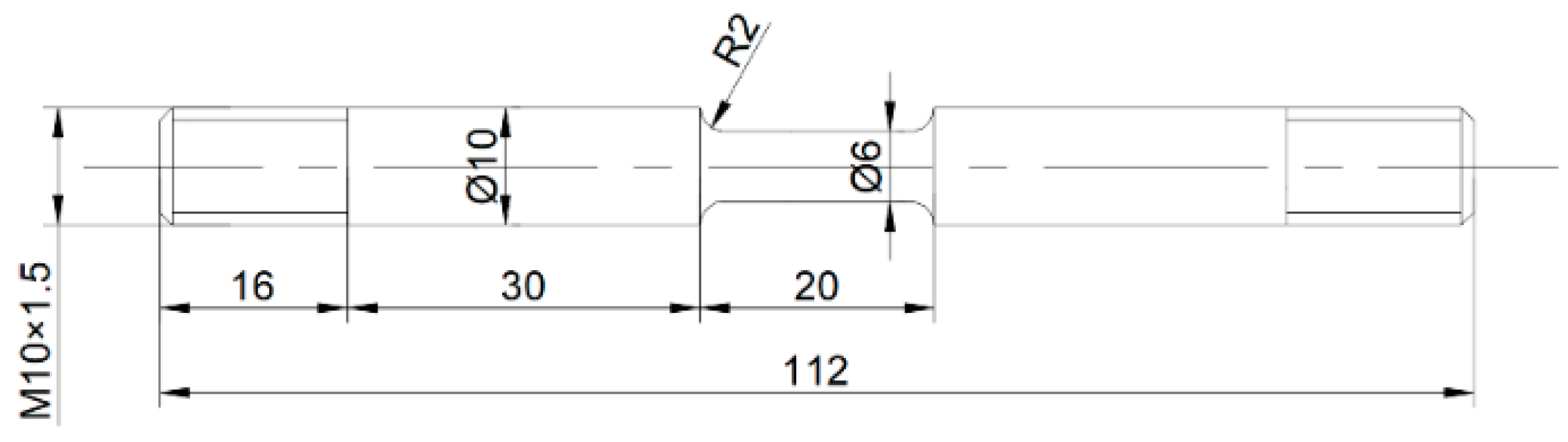
Figure 2.
Thermal simulation experiment process roadmap.
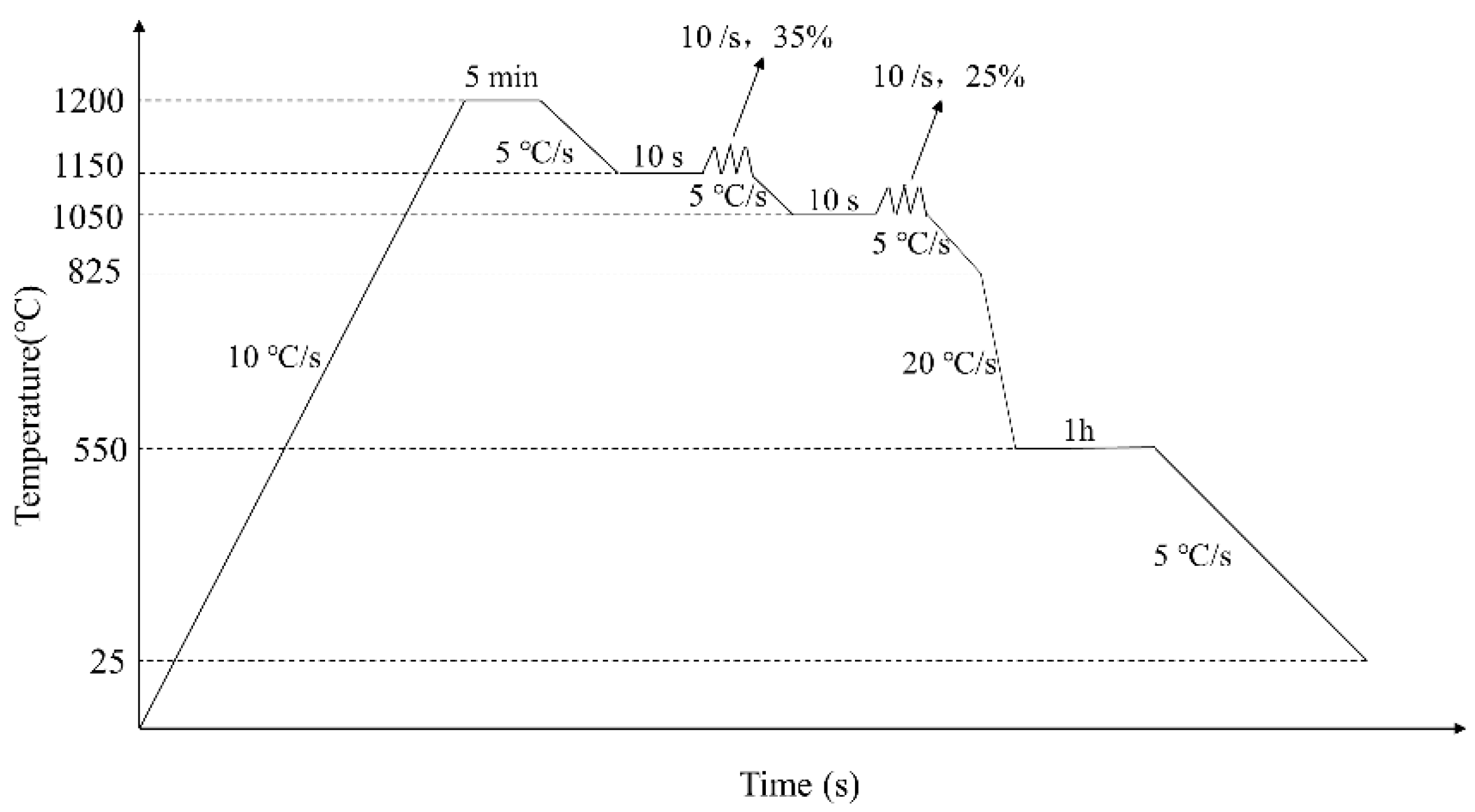
Figure 3.
Grain size distribution of each specimen in orthogonal experiments. (a) 1; (b) 2; (c) 3; (d) 4; (e) 5; (f) 6; (g) 7; (h) 8; (i) 9; (j) 10; (k) 11; (l) 12; (m) 13; (n) 14; (o) 15; (p) 16.
Figure 3.
Grain size distribution of each specimen in orthogonal experiments. (a) 1; (b) 2; (c) 3; (d) 4; (e) 5; (f) 6; (g) 7; (h) 8; (i) 9; (j) 10; (k) 11; (l) 12; (m) 13; (n) 14; (o) 15; (p) 16.
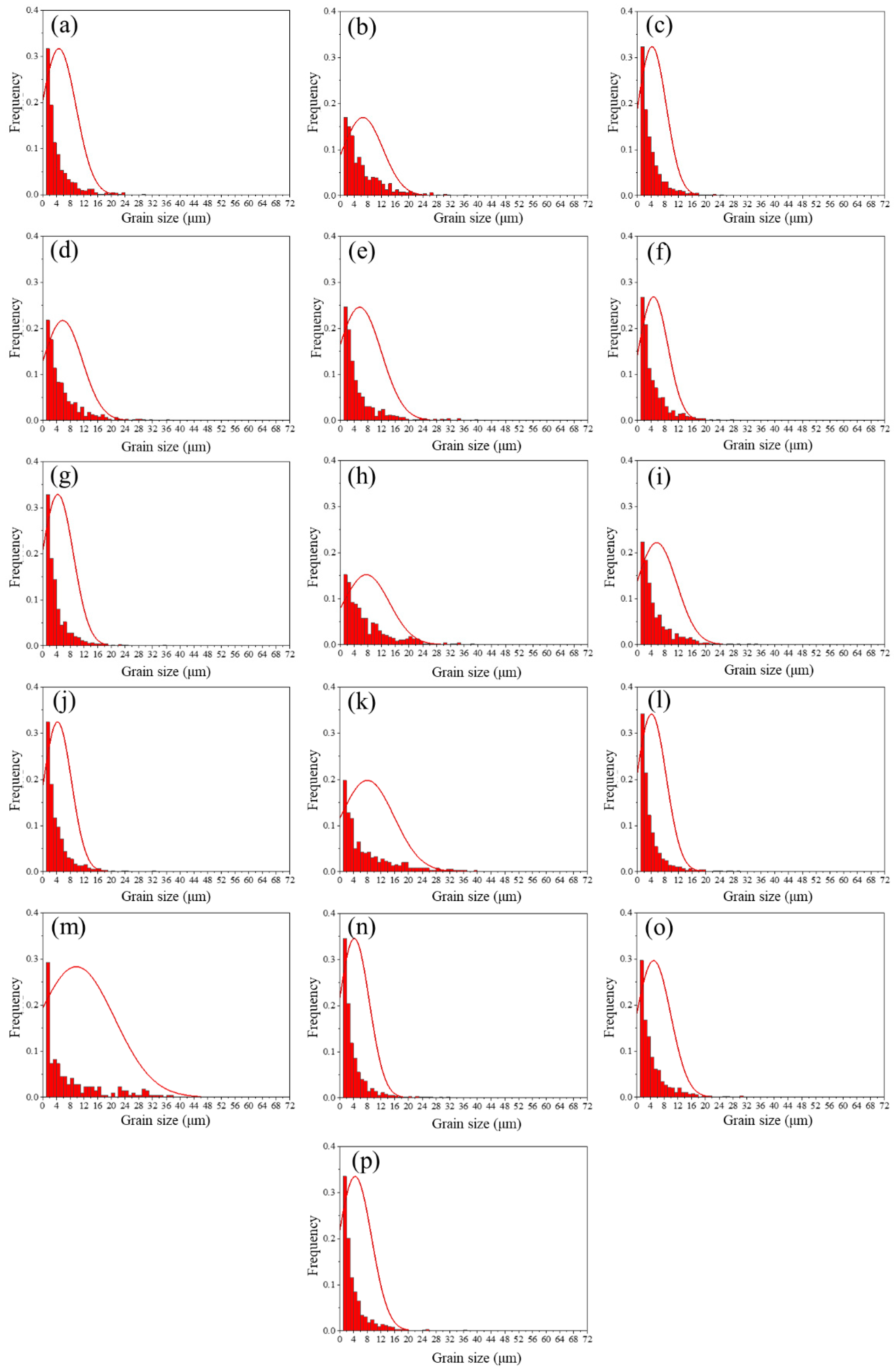
Figure 4.
Trend plot of grain size variation with cooling process.

Figure 5.
KAM distribution of each specimen in orthogonal experiments. (a) 1; (b) 2; (c) 3; (d) 4; (e) 5; (f) 6; (g) 7; (h) 8; (i) 9; (j) 10; (k) 11; (l) 12; (m) 13; (n) 14; (o) 15; (p) 16.
Figure 5.
KAM distribution of each specimen in orthogonal experiments. (a) 1; (b) 2; (c) 3; (d) 4; (e) 5; (f) 6; (g) 7; (h) 8; (i) 9; (j) 10; (k) 11; (l) 12; (m) 13; (n) 14; (o) 15; (p) 16.
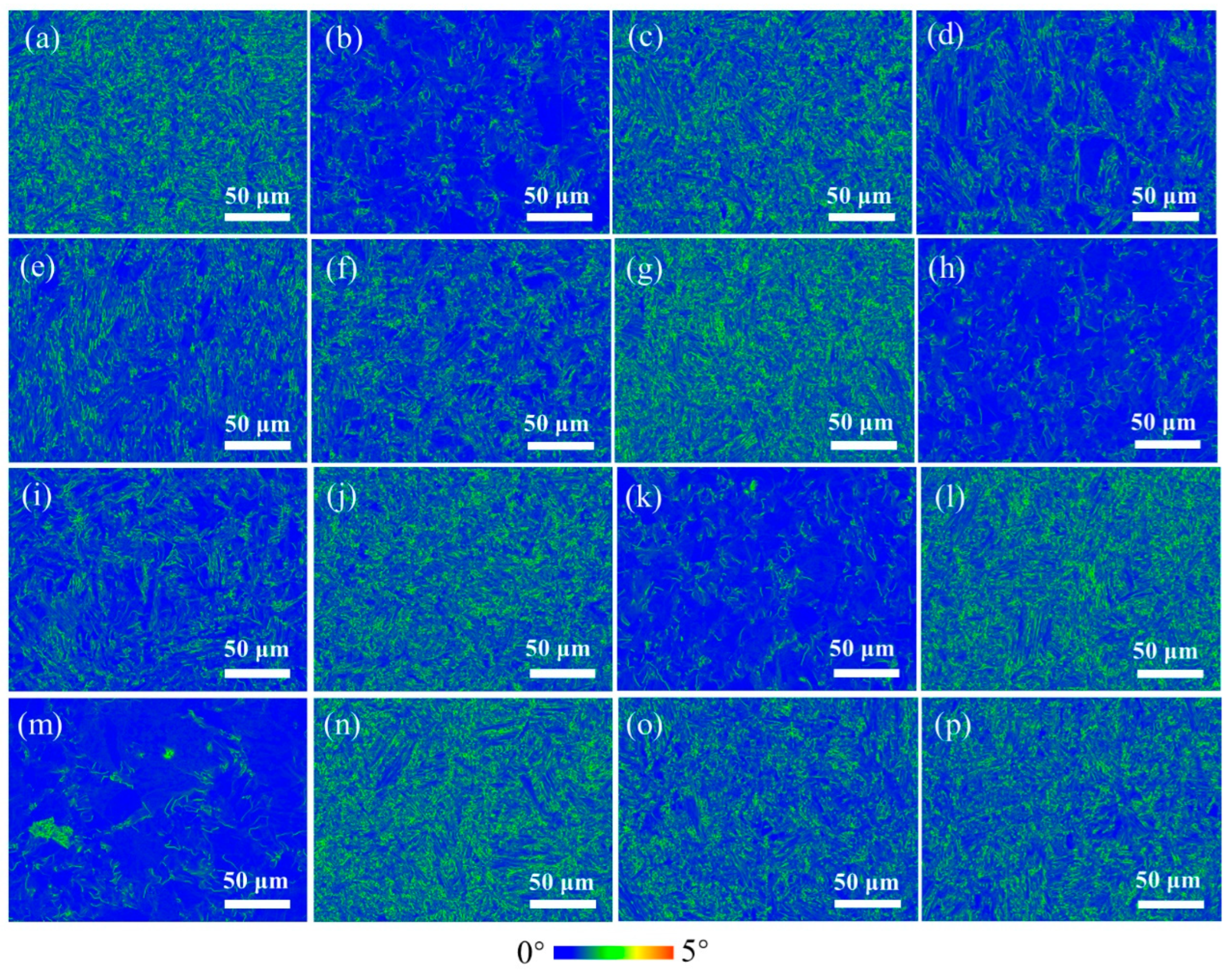
Figure 6.
Trend plot of KAM variation with cooling process.
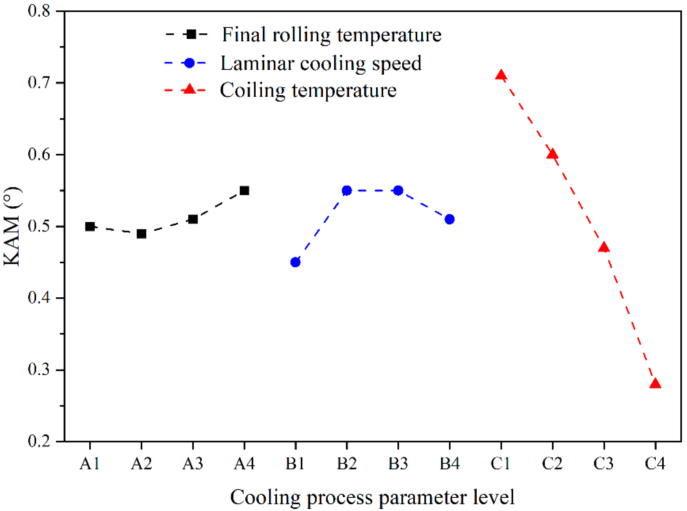
Figure 7.
Evaluation indicators of gray correlation analysis optimization scheme. (a) Grain size distribution; (b) KAM distribution.
Figure 7.
Evaluation indicators of gray correlation analysis optimization scheme. (a) Grain size distribution; (b) KAM distribution.
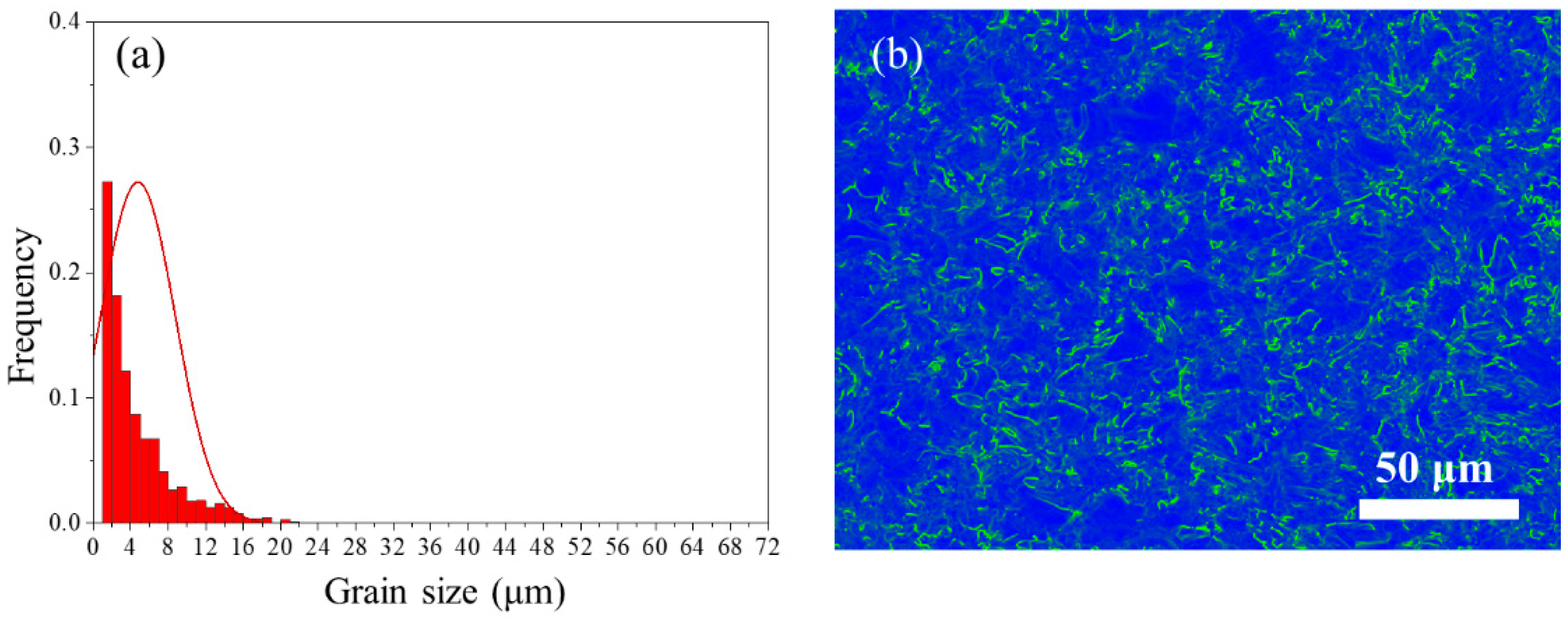
Figure 8.
Evaluation indicators of practical production process scheme. (a) Grain size distribution; (b) KAM distribution.
Figure 8.
Evaluation indicators of practical production process scheme. (a) Grain size distribution; (b) KAM distribution.
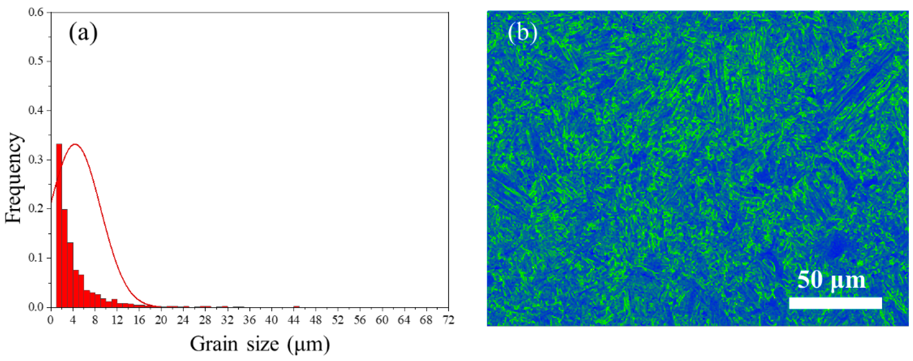
Figure 9.
Comparison of evaluation indicators between optimized and actual production process scheme.
Figure 9.
Comparison of evaluation indicators between optimized and actual production process scheme.


Table 1.
Chemical composition of test steel (wt.%).
| Elements | C | Si | Mn | Al | Nb + V + Ti | Fe |
|---|---|---|---|---|---|---|
| Composition | 0.08 | 0.15 | 1.25 | 0.03 | 0.08 | Rest |
Table 2.
Factors and levels of orthogonal experiments.
| Levels | Factors | ||
|---|---|---|---|
| A (°C) | B (°C/s) | C (°C) | |
| 1 | 825 | 20 | 550 |
| 2 | 850 | 30 | 575 |
| 3 | 875 | 40 | 600 |
| 4 | 900 | 50 | 625 |
Table 3.
Orthogonal experimental results of grain size.
| Numbers | Factors | Targets | ||
|---|---|---|---|---|
| A (°C) | B (°C/s) | C (°C) | D (μm) | |
| 1 | 825 | 20 | 550 | 4.7 |
| 2 | 825 | 30 | 625 | 6.6 |
| 3 | 825 | 40 | 575 | 4.3 |
| 4 | 825 | 50 | 600 | 5.8 |
| 5 | 850 | 20 | 575 | 5.6 |
| 6 | 850 | 30 | 600 | 4.7 |
| 7 | 850 | 40 | 550 | 4.4 |
| 8 | 850 | 50 | 625 | 7.6 |
| 9 | 875 | 20 | 600 | 5.7 |
| 10 | 875 | 30 | 575 | 4.3 |
| 11 | 875 | 40 | 625 | 8.1 |
| 12 | 875 | 50 | 550 | 4.2 |
| 13 | 900 | 20 | 625 | 9.8 |
| 14 | 900 | 30 | 550 | 4.3 |
| 15 | 900 | 40 | 600 | 5.0 |
| 16 | 900 | 50 | 575 | 4.5 |
Table 4.
Range of effect of cooling process on grain size.
| Factors | Mean Grain Size at Different Levels (μm) | Range (μm) | Sort | |||
|---|---|---|---|---|---|---|
| 1 | 2 | 3 | 4 | |||
| A | 5.4 | 5.6 | 5.6 | 5.9 | 0.5 | 3 |
| B | 6.5 | 5.0 | 5.5 | 5.5 | 1.5 | 2 |
| C | 4.4 | 4.7 | 5.3 | 8.0 | 3.6 | 1 |
Table 5.
Orthogonal experimental results of KAM.
| Numbers | Factors | Targets | ||
|---|---|---|---|---|
| A (°C) | B (°C/s) | C (°C) | E (°) | |
| 1 | 825 | 20 | 550 | 0.67 |
| 2 | 825 | 30 | 625 | 0.31 |
| 3 | 825 | 40 | 575 | 0.63 |
| 4 | 825 | 50 | 600 | 0.40 |
| 5 | 850 | 20 | 575 | 0.47 |
| 6 | 850 | 30 | 600 | 0.49 |
| 7 | 850 | 40 | 550 | 0.72 |
| 8 | 850 | 50 | 625 | 0.29 |
| 9 | 875 | 20 | 600 | 0.41 |
| 10 | 875 | 30 | 575 | 0.66 |
| 11 | 875 | 40 | 625 | 0.28 |
| 12 | 875 | 50 | 550 | 0.70 |
| 13 | 900 | 20 | 625 | 0.25 |
| 14 | 900 | 30 | 550 | 0.73 |
| 15 | 900 | 40 | 600 | 0.57 |
| 16 | 900 | 50 | 575 | 0.63 |
Table 6.
Range of effect of cooling process on KAM.
| Factors | Mean KAM at Different Levels (°) | Range (°) | Sort | |||
|---|---|---|---|---|---|---|
| 1 | 2 | 3 | 4 | |||
| A | 0.50 | 0.49 | 0.51 | 0.55 | 0.06 | 3 |
| B | 0.45 | 0.55 | 0.55 | 0.51 | 0.10 | 2 |
| C | 0.71 | 0.60 | 0.47 | 0.28 | 0.43 | 1 |
Table 7.
Normalization results for response objectives in gray correlation optimization schemes.
| Numbers | Experimental Data | Normalized Data | ||
|---|---|---|---|---|
| D (μm) | E (°) | D | E | |
| 1 | 4.7 | 0.67 | 0.911 | 0.125 |
| 2 | 6.6 | 0.31 | 0.571 | 0.875 |
| 3 | 4.3 | 0.63 | 0.982 | 0.208 |
| 4 | 5.8 | 0.40 | 0.714 | 0.688 |
| 5 | 5.6 | 0.47 | 0.750 | 0.542 |
| 6 | 4.7 | 0.49 | 0.911 | 0.500 |
| 7 | 4.4 | 0.72 | 0.964 | 0.021 |
| 8 | 7.6 | 0.29 | 0.393 | 0.917 |
| 9 | 5.7 | 0.41 | 0.732 | 0.667 |
| 10 | 4.3 | 0.66 | 0.982 | 0.146 |
| 11 | 8.1 | 0.28 | 0.304 | 0.938 |
| 12 | 4.2 | 0.70 | 1.000 | 0.063 |
| 13 | 9.8 | 0.25 | 0.000 | 1.000 |
| 14 | 4.3 | 0.73 | 0.982 | 0.000 |
| 15 | 5.0 | 0.57 | 0.857 | 0.333 |
| 16 | 4.5 | 0.63 | 0.946 | 0.208 |
Table 8.
Calculation results of gray correlation coefficient and gray correlation degree.
| Numbers | Gray Correlation Coefficient | Gray Correlation Degree | |
|---|---|---|---|
| D | E | ||
| 1 | 0.848 | 0.364 | 0.606 |
| 2 | 0.538 | 0.800 | 0.669 |
| 3 | 0.966 | 0.387 | 0.676 |
| 4 | 0.636 | 0.615 | 0.626 |
| 5 | 0.667 | 0.522 | 0.594 |
| 6 | 0.848 | 0.500 | 0.674 |
| 7 | 0.933 | 0.338 | 0.636 |
| 8 | 0.452 | 0.857 | 0.654 |
| 9 | 0.651 | 0.600 | 0.626 |
| 10 | 0.966 | 0.369 | 0.667 |
| 11 | 0.418 | 0.889 | 0.653 |
| 12 | 1.000 | 0.348 | 0.674 |
| 13 | 0.333 | 1.000 | 0.667 |
| 14 | 0.966 | 0.333 | 0.649 |
| 15 | 0.778 | 0.429 | 0.603 |
| 16 | 0.903 | 0.387 | 0.645 |
Table 9.
Mean gray correlation degree at different levels of each factor.
| Factors | Mean Gray Correlation Degree at Different Levels | |||
|---|---|---|---|---|
| 1 | 2 | 3 | 4 | |
| A | 0.644 | 0.640 | 0.655 | 0.641 |
| B | 0.623 | 0.665 | 0.642 | 0.650 |
| C | 0.641 | 0.646 | 0.632 | 0.661 |
Disclaimer/Publisher’s Note: The statements, opinions and data contained in all publications are solely those of the individual author(s) and contributor(s) and not of MDPI and/or the editor(s). MDPI and/or the editor(s) disclaim responsibility for any injury to people or property resulting from any ideas, methods, instructions or products referred to in the content. |
© 2024 by the authors. Licensee MDPI, Basel, Switzerland. This article is an open access article distributed under the terms and conditions of the Creative Commons Attribution (CC BY) license (https://creativecommons.org/licenses/by/4.0/).
Share and Cite
MDPI and ACS Style
Xue, R.; Fei, A. Multi-Objective Optimization of Low-Alloy Hot-Rolled Strip Cooling Process Based on Gray Correlation Analysis. Metals 2024, 14, 246. https://doi.org/10.3390/met14020246
AMA Style
Xue R, Fei A. Multi-Objective Optimization of Low-Alloy Hot-Rolled Strip Cooling Process Based on Gray Correlation Analysis. Metals. 2024; 14(2):246. https://doi.org/10.3390/met14020246
Chicago/Turabian StyleXue, Rundong, and Aigeng Fei. 2024. "Multi-Objective Optimization of Low-Alloy Hot-Rolled Strip Cooling Process Based on Gray Correlation Analysis" Metals 14, no. 2: 246. https://doi.org/10.3390/met14020246
Note that from the first issue of 2016, this journal uses article numbers instead of page numbers. See further details here.