
Prediction of Activity Coefficients and Osmotic Coefficient of Electrolyte Solutions Containing Rb+ by the Electrolyte Molecular Interaction Volume Model and the Electrolyte Molecular Interaction Volume Model-Energy Term
Abstract
:1. Introduction
2. Thermodynamic Modelling Framework
2.1. Long-Range Terms
2.2. eMIVM Short-Range Items
2.3. eMIVM-ET Short-Range Items
2.4. Radii and Molar Volumes of Ions in Aqueous Solution
3. Results and Comparison
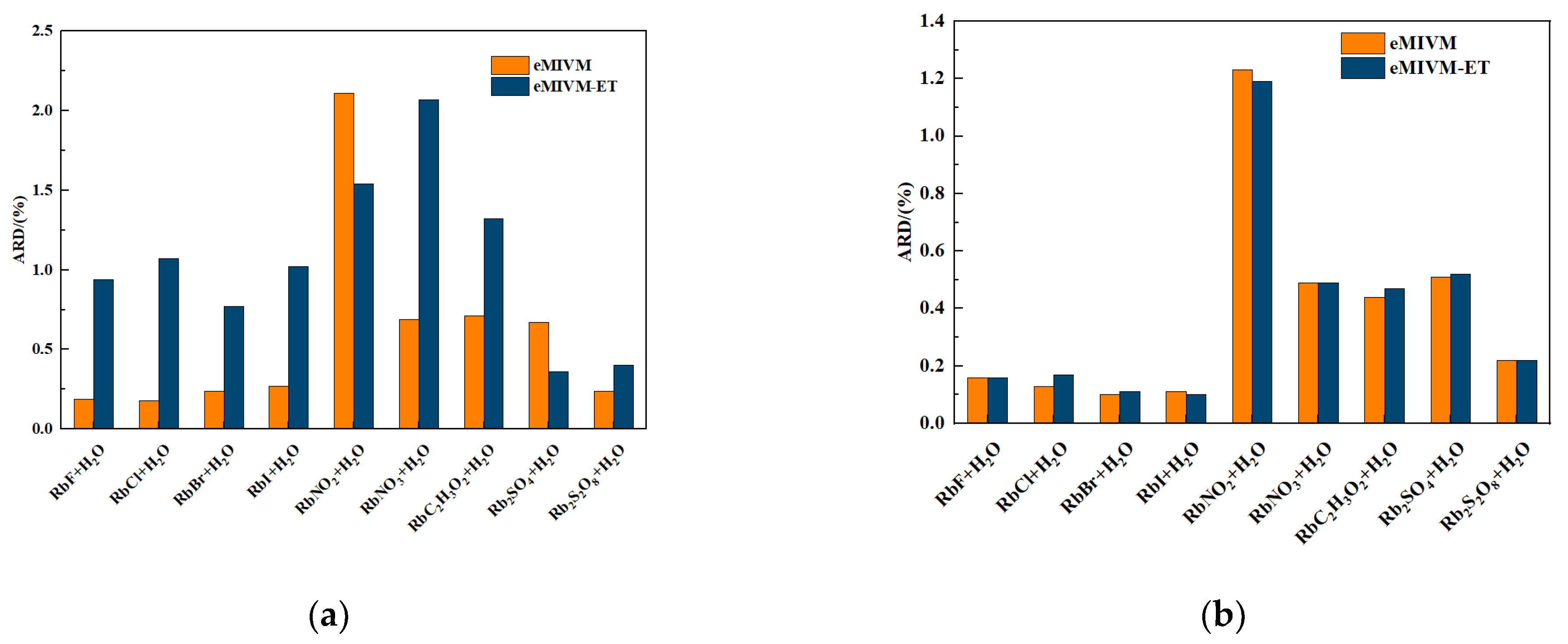
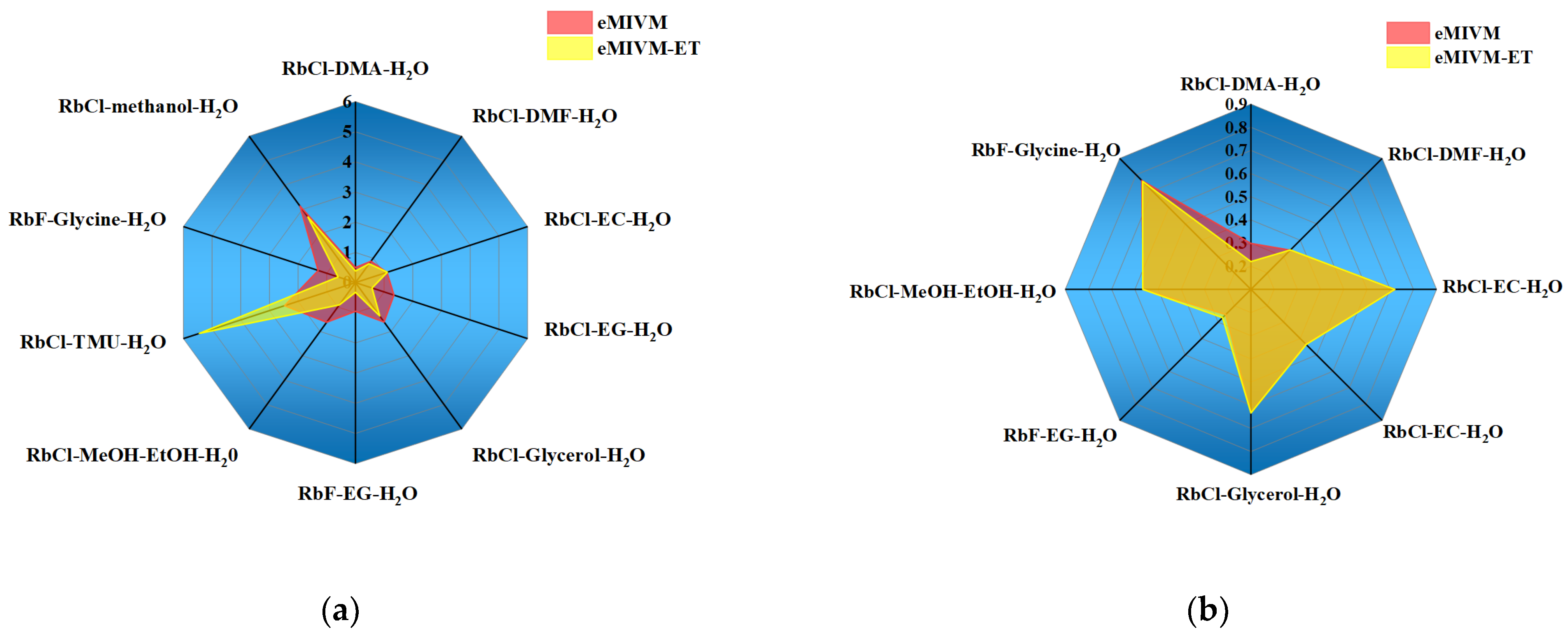
3.1. Activity-Coefficient Fitting
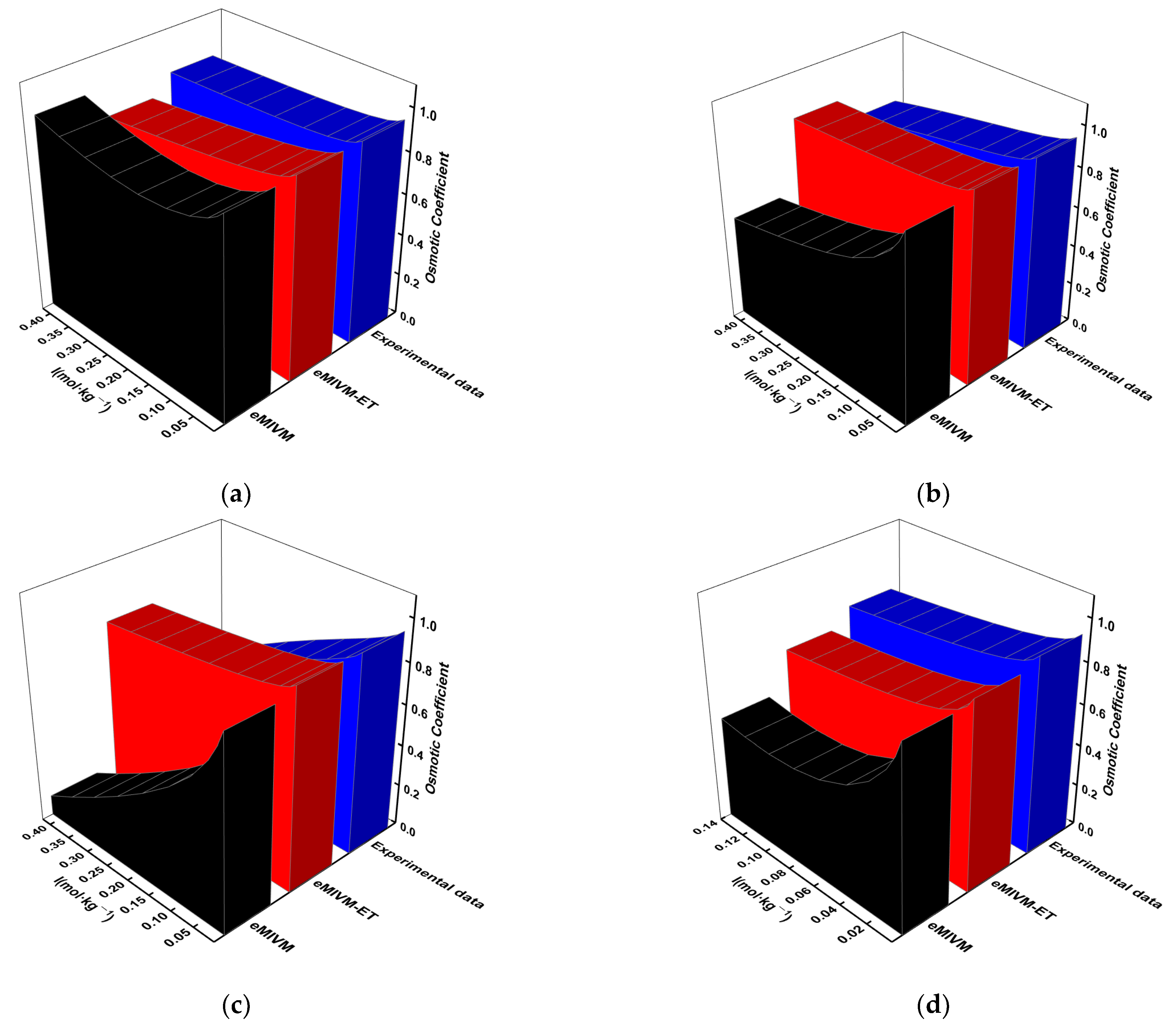
3.2. Osmotic-Coefficient Fitting
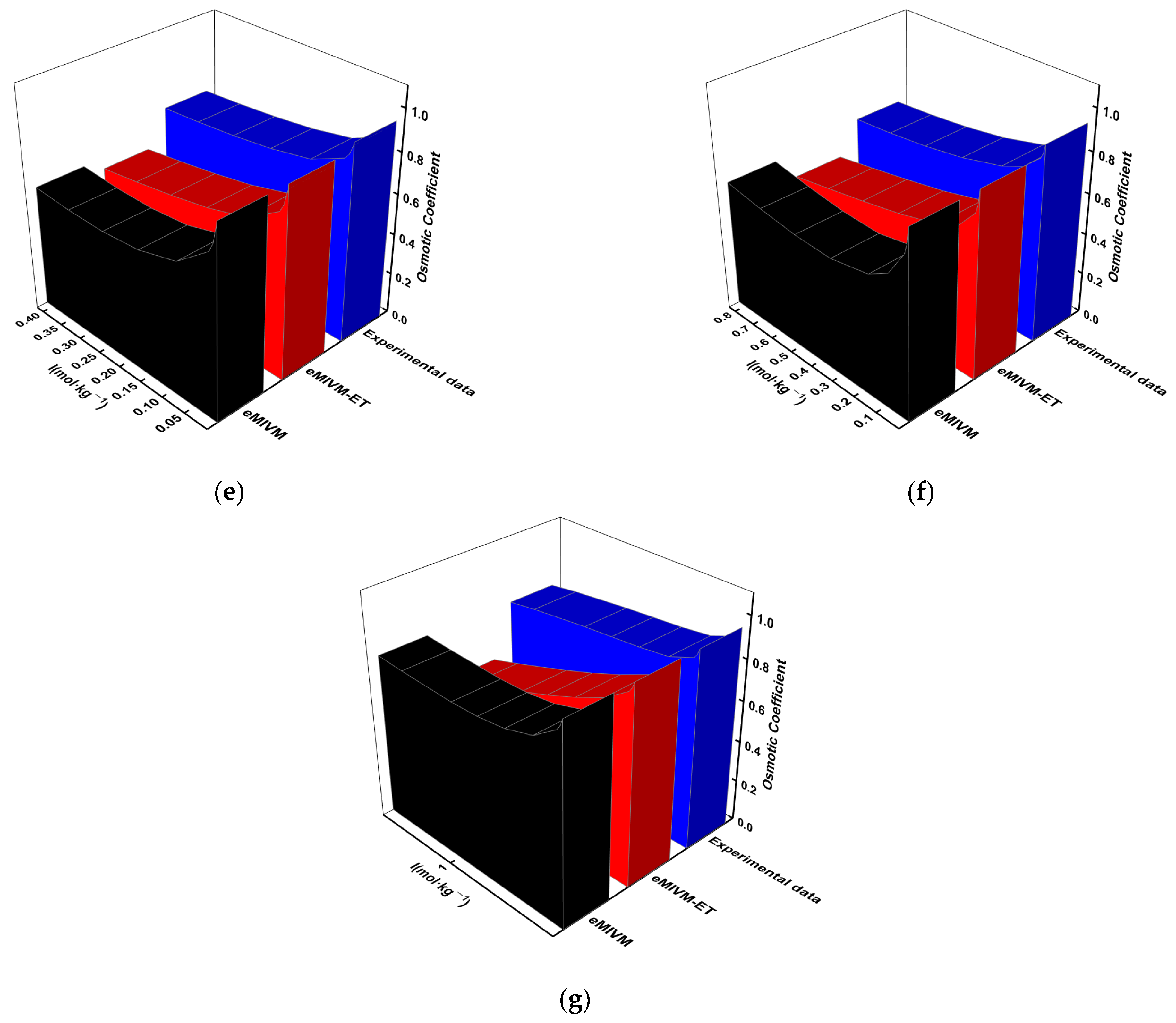
3.3. Model Predictions
4. Conclusions
- In fitting activity and osmotic coefficients to single-electrolyte solutions containing Rb+, the eMIVM-ET model outperforms the eMIVM model in organic electrolyte solutions. In contrast, the eMIVM model fits better in aqueous electrolyte solutions.
- In the case of the monoelectrolyte solution of Rb+, there is minimal variation in the results of binary parameter fitting for the same system at different temperatures. This suggests that the accuracy of predictions remains unaffected by temperature.
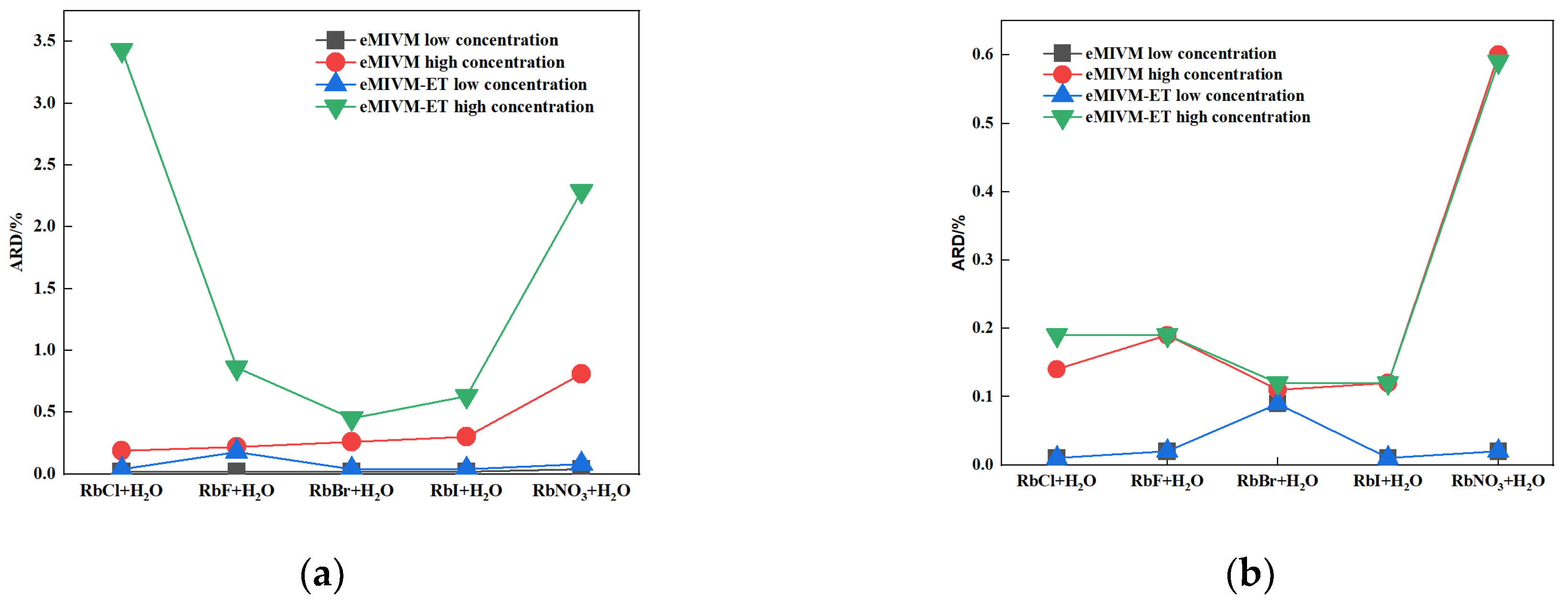
- In the fitting of activity coefficients and osmotic coefficients of electrolyte solutions for the same system, the average deviation and the average relative error are more minor in low-concentration solutions than in high-concentration solutions; i.e., the lower the concentration, the better the fit.
- In predicting activity coefficients and osmotic coefficients of two-electrolyte solutions, the prediction of the eMIVM-ET model is better than that of the eMIVM model. These calculations can provide alternative models for the future prediction of the thermodynamics of multi-component systems for better guidance for industrial production.
Author Contributions
Funding
Data Availability Statement
Acknowledgments
Conflicts of Interest
References
- Ramkrishna, D.; Braatz, R.D. Whither chemical engineering? AIChE J. 2022, 68, e17829. [Google Scholar] [CrossRef]
- Horio, M.; Clift, R. Chemical engineering for the Anthropocene. Can. J. Chem. Eng. 2023, 101, 295–308. [Google Scholar] [CrossRef]
- Chagnes, A. Advances in Hydrometallurgy. Metals 2019, 9, 211. [Google Scholar] [CrossRef]
- Han, K.N.; Kim, R.; Kim, J. Recent Advancements in Hydrometallurgy: Solubility and Separation. Trans. Indian Inst. Met. 2023, 1–13. [Google Scholar] [CrossRef]
- Li, Z.; Liu, H. Study on electrochemical properties of lead calcium tin anode for hydrometallurgy. Alex. Eng. J. 2023, 82, 389–395. [Google Scholar] [CrossRef]
- Ding, T.; Zheng, M.; Nie, Z.; Ma, L.; Ye, C.; Wu, Q.; Zhao, Y.; Yang, D.; Wang, K. Impact of Regional Climate Change on the Development of Lithium Resources in Zabuye Salt Lake, Tibet. Front. Earth Sci. 2022. [Google Scholar] [CrossRef]
- Bekri, E.S.; Kokkoris, I.P.; Christodoulou, C.S.; Sophocleous-Lemonari, A.; Dimopoulos, P. Management Implications at a Protected, Peri-Urban, Salt Lake Ecosystem: The Case of Larnaca’s Salt Lakes (Cyprus). Land 2023, 12, 1781. [Google Scholar] [CrossRef]
- Italiano, F.; Solecki, A.; Martinelli, G.; Wang, Y.; Zheng, G. New Applications in Gas Geochemistry. Geofluids 2020, 2020, 4976190. [Google Scholar] [CrossRef]
- Fernandez-Suarez, J.; Sanchez Martinez, S.; Fuenlabrada, J.M. Geochemistry in earth sciences: A brief overview. J. Iber. Geol. 2021, 47, 3–13. [Google Scholar] [CrossRef]
- Deng, H.; Li, L.; Kim, J.J.; Ling, F.T.; Beckingham, L.E.; Wammer, K.H. Bridging environmental geochemistry and hydrology. J. Hydrol. 2022, 613, 128448. [Google Scholar] [CrossRef]
- Franikovi-Bilinski, S.; Sakan, S. Geochemistry of Water and Sediment. Water 2021, 13, 693. [Google Scholar] [CrossRef]
- Lu, B.; Ru, N.; Duan, J.; Li, Z.; Qu, J. In-Plane Porous Graphene: A Promising Anode Material with High Ion Mobility and Energy Storage for Rubidium-Ion Batteries. ACS Omega 2023. [Google Scholar] [CrossRef]
- Smith, J.P.; Boyd, T.J.; Cragan, J.; Ward, M.C. Dissolved rubidium to strontium ratio as a conservative tracer for wastewater effluent-sourced contaminant inputs near a major urban wastewater treatment plant. Water Res. 2021, 205, 117691. [Google Scholar] [CrossRef] [PubMed]
- Lau, S.; Atakan, B. Combined Thermogravimetric Determination of Activity Coefficients and Binary Diffusion Coefficients—A New Approach Applied to Ferrocene/n-Tetracosane Mixtures. J. Chem. Eng. Data 2019, 65, 1211–1221. [Google Scholar] [CrossRef]
- Noguchi, D.; Takeda, O.; Abe, T.; Zhu, H.; Sugimoto, S. Determination of activity of RE (RE = Nd and Dy) in molten RE-Fe-B alloys by the electromotive force method. Thermochim. Acta Int. J. Concerned Broader Asp. Thermochem. Its Appl. Chem. Probl. 2022, 709, 179161. [Google Scholar] [CrossRef]
- El Fadel, W.; El Hantati, S.; Nour, Z.; Dinane, A.; Samaouali, A.; Messnaoui, B. Experimental Determination of Osmotic Coefficient and Salt Solubility of System NH4NO3–NH4H2PO4–H2O and Their Correlation and Prediction with the Pitzer–Simonson–Clegg Model. Ind. Eng. Chem. Res. 2023, 62, 17986–17996. [Google Scholar] [CrossRef]
- Passamonti, F.J.; de Chialvo MR, G.; Chialvo, A.C. Evaluation of the activity coefficients of ternary molecular solutions from osmotic coefficient data. Fluid Phase Equilibria 2022, 559, 113464. [Google Scholar] [CrossRef]
- Zafarani-Moattar, M.T.; Mokhtarpour, M.; Faraji, S. Osmotic Coefficients of Gabapentin Drug in Aqueous Solutions of Deep Eutectic Solvents: Experimental Measurements and Thermodynamic Modeling. J. Chem. Eng. Data 2023, 68, 1663–1672. [Google Scholar]
- McMillan Jr, W.G.; Mayer, J.E. The statistical thermodynamics of multicomponent systems. J. Chem. Phys. 1945, 13, 276–305. [Google Scholar] [CrossRef]
- Pitzer, K.S. Electrolyte theory-improvements since Debye and Hueckel. Acc. Chem. Res. 1977, 10, 371–377. [Google Scholar] [CrossRef]
- Xiao, T.; Zhou, Y. Fast Calculation of Electrostatic Solvation Free Energy in Simple Ionic Fluids Using an Energy-Scaled Debye–Hückel Theory. J. Phys. Chem. Lett. 2021, 12, 6262–6268. [Google Scholar] [CrossRef] [PubMed]
- Pitzer, K.S. Thermodynamics of electrolytes. I. Theoretical basis and general equations. J. Phys. Chem. 1973, 77, 268–277. [Google Scholar] [CrossRef]
- Pitzer, K.S.; Mayorga, G. Thermodynamics of electrolytes. II. Activity and osmotic coefficients for strong electrolytes with one or both ions univalent. J. Phys. Chem. 1973, 7, 2300–2308. [Google Scholar] [CrossRef]
- Pitzer, K.S.; Kim, J.J. Thermodynamics of electrolytes. IV. Activity and osmotic coefficients for mixed electrolytes. J. Am. Chem. Soc. 1974, 96, 5701–5707. [Google Scholar] [CrossRef]
- Das, B. Pitzer ion interaction parameters of single aqueous electrolytes at 25 °C. J. Solut. Chem. 2004, 33, 33–45. [Google Scholar] [CrossRef]
- Sun, L.; Lei, Q.; Peng, B.; Kontogeorgis, G.M.; Liang, X. An analysis of the parameters in the Debye-Hückel theory. Fluid Phase Equilibria 2022, 556, 113398. [Google Scholar] [CrossRef]
- Michelsen, M.L.; Mollerup, J.M. Thermodynamic Models: Fundamentals & Computational Aspects; Tie-Line Publications: Holte, Denmark, 2007. [Google Scholar]
- Kunz, W. (Ed.) Specific Ion Effects; World Scientific: Hackensack, NJ, USA, 2010. [Google Scholar]
- Rowland, D.; Königsberger, E.; Hefter, G.; May, P.M. Aqueous electrolyte solution modelling: Some limitations of the Pitzer equations. Appl. Geochem. 2015, 55, 170–183. [Google Scholar] [CrossRef]
- Voigt, W. Chemistry of salts in aqueous solutions: Applications, experiments, and theory. Pure Appl. Chem. 2011, 83, 1015–1030. [Google Scholar] [CrossRef]
- Chen, C.C.; Bokis, C.P.; Mathias, P. Segment-based excess Gibbs energy model for aqueous organic electrolytes. AIChE J. 2001, 47, 2593–2602. [Google Scholar] [CrossRef]
- Chen, C.; Britt, H.I.; Boston, J.F.; Evans, L.B. Local composition model for excess Gibbs energy of electrolyte systems. Part I: Single solvent, single completely dissociated electrolyte systems. AIChE J. 1982, 28, 588–596. [Google Scholar] [CrossRef]
- Chen, C.C. Some recent developments in process simulation for reactive chemical systems. Pure Appl. Chem. 1987, 59, 1177–1188. [Google Scholar] [CrossRef]
- Thomsen, K.; Rasmussen, P.; Gani, R. Correlation and prediction of thermal properties and phase behaviour for a class of aqueous electrolyte systems. Chem. Eng. Sci. 1996, 51, 3675–3683. [Google Scholar] [CrossRef]
- Thomsen, K.; Rasmussen, P. Modeling of vapor–liquid–solid equilibrium in gas–aqueous electrolyte systems. Chem. Eng. Sci. 1999, 54, 1787–1802. [Google Scholar] [CrossRef]
- Thomsen, K. Modeling electrolyte solutions with the extended universal quasichemical (UNIQUAC) model. Pure Appl. Chem. 2005, 77, 531–542. [Google Scholar] [CrossRef]
- Wang, P.; Anderko, A.; Young, R.D. A speciation-based model for mixed-solvent electrolyte systems. Fluid Phase Equilibria 2002, 203, 141–176. [Google Scholar] [CrossRef]
- Kosinski, J.J.; Wang, P.; Springer, R.D.; Anderko, A. Modeling acid–base equilibria and phase behavior in mixed-solvent electrolyte systems. Fluid Phase Equilibria 2007, 256, 34–41. [Google Scholar] [CrossRef]
- Jaworski, Z.; Czernuszewicz, M.; Gralla, Ł. A comparative study of thermodynamic electrolyte models applied to the Solvay soda system. Chem. Process Eng. 2011, 32, 135–154. [Google Scholar] [CrossRef]
- Zhang, C.; Xing, Y.; Tao, D. A Two-Parameter Theoretical Model for Predicting the Activity and Osmotic Coefficients of Aqueous Electrolyte Solutions. J. Solut. Chem. 2020, 49, 659–694. [Google Scholar] [CrossRef]
- Pitzer, K.S. Electrolytes. From dilute solutions to fused salts. J. Am. Chem. Soc. 1980, 102, 2902–2906. [Google Scholar] [CrossRef]
- Zheng, S.; Xu, C.; Tao, D.P. Prediction of activity coefficients for Cu2+-containing electrolyte solutions. Nonferrous Met. Eng. 2023, 13, 59–68. [Google Scholar]
- Zheng, S.; Xu, C.; Lu, Y.; Tao, D. Prediction of Thermodynamic Properties of Ni2+, Co2+, Cu2+ Electrolyte Solutions by eMIVM-ET. J. Solut. Chem. 2023, 52, 1273–1288. [Google Scholar] [CrossRef]
- Tao, D.P. A new model of thermodynamics of liquid mixtures and its application to liquid alloys. Thermochim. Acta 2000, 363, 105–113. [Google Scholar] [CrossRef]
- Simonson, J.M.; Pitzer, K.S. Thermodynamics of multicomponent, miscible ionic systems: The system lithium nitrate-potassium nitrate-water. J. Phys. Chem. 1986, 90, 3009–3013. [Google Scholar] [CrossRef]
- Tao, D.P. The universal characteristics of a thermodynamic model to conform to the Gibbs-Duhem equation. Sci. Rep. 2016, 6, 35792. [Google Scholar] [CrossRef]
- Marcus, Y. Ionic volumes in solution. Biophys. Chem. 2006, 124, 200–207. [Google Scholar] [CrossRef]
- Haghtalab, A.; Peyvandi, K. Electrolyte-UNIQUAC-NRF model for the correlation of the mean activity coefficient of electrolyte solutions. Fluid Phase Equilibria 2009, 281, 163–171. [Google Scholar] [CrossRef]
- Li, F.; Li, W. Metallurgy and Thermodynamics of Materials; Metallurgical Industry Press: Beijing, China, 2012. [Google Scholar]
- Marcus, Y. Thermodynamics of solvation of ions. Part 6—The standard partial molar volumes of aqueous ions at 298.15 K. J. Chem. Soc. Faraday Trans. 1993, 89, 713–718. [Google Scholar] [CrossRef]
- Longhi, P.; Mussini, T.; Osimani, C. Standard potentials of the rubidium amalgam electrode, and thermodynamic functions for dilute rubidium amalgams and for aqueous rubidium chloride. J. Chem. Thermodyn. 1974, 6, 227–235. [Google Scholar] [CrossRef]
- Palmer, D.A.; Rard, J.A.; Clegg, S.L. Isopiestic determination of the osmotic and activity coefficients of Rb2SO4 (aq) and Cs2SO 4 (aq) at T = (298.15 and 323.15) K, and representation with an extended ion-interaction (Pitzer) model. J. Chem. Thermodyn. 2002, 34, 63–102. [Google Scholar] [CrossRef]
- Hamer, W.J.; Wu, Y.C. Osmotic Coefficients and Mean Activity Coefficients of Uni-univalent Electrolytes in Water at 25 °C. J. Phys. Chem. Ref. Data 1972, 1, 1047–1100. [Google Scholar] [CrossRef]
- Partanen, J.I. Re-evaluation of the thermodynamic activity quantities in aqueous solutions of silver nitrate, alkali metal fluorides and nitrites, and dihydrogen phosphate, dihydrogen arsenate, and thiocyanate salts with sodium and potassium ions at 25 °C. J. Chem. Eng. Data 2011, 56, 2044–2062. [Google Scholar] [CrossRef]
- Robinson, R.A.; Stokes, R.H. Electrolyte Solutions; Courier Corporation: North Chelmsford, MA, USA, 2002. [Google Scholar]
- Goldberg, R.N. Evaluated activity and osmotic coefficients for aqueous solutions: Bi-univalent compounds of zinc, cadmium, and ethylene bis (trimethylammonium) chloride and iodide. J. Phys. Chem. Ref. Data 1981, 10, 1–56. [Google Scholar] [CrossRef]
- Lu, J.; Li, S.N.; Zhai, Q.; Jiang, Y.; Hu, M. Investigating thermodynamic properties of the ternary systems of MCl (M = K, Rb, Cs) with aqueous mixed solvent: N, N-dimethylacetamide. J. Mol. Liq. 2013, 178, 15–19. [Google Scholar] [CrossRef]
- Wang, L.; Li, S.; Zhai, Q.; Zhang, H.; Jiang, Y.; Zhang, W.; Hu, M. Thermodynamic Study of RbCl or CsCl in the Mixed Solvent DMF + H2O by Potentiometric Measurements at 298.15 K. J. Chem. Eng. Data 2010, 55, 4699–4703. [Google Scholar] [CrossRef]
- Hao, X.; Li, S.; Zhai, Q.; Jiang, Y.; Hu, M. Phase equilibrium and activity coefficients in ternary systems at 298.15 K: RbCl/CsCl + ethylene carbonate + water. J. Chem. Thermodyn. 2016, 98, 309–316. [Google Scholar] [CrossRef]
- Tang, J.; Ma, Y.; Li, S.; Zhai, Q.; Jiang, Y.; Hu, M. Activity Coefficients of RbCl in Ethylene Glycol + Water and Glycerol + Water Mixed Solvents at 298.15 K. J. Chem. Eng. Data 2011, 56, 2356–2361. [Google Scholar] [CrossRef]
- Wang, L.; Li, S.; Zhai, Q.; Jiang, Y.; Hu, M. Activity Coefficients of RbF or CsF in the Ethene Glycol + Water System by Potentiometric Measurements at 298.15 K. J. Chem. Eng. Data 2011, 56, 4416–4421. [Google Scholar] [CrossRef]
- Du, Y.; Li, S.N.; Zhai, Q.; Jiang, Y.; Hu, M. Activity coefficients in quaternary systems at 298.15 K: RbCl + MeOH + EtOH + H2O and CsCl + MeOH + EtOH + H2O systems. J. Chem. Eng. Data 2013, 58, 2545–2551. [Google Scholar] [CrossRef]
- Cao, X.; Chang, Y.; Li, S.; Zhai, Q.; Jiang, Y.; Hu, M. Thermodynamic properties of MCl (M = Na, K, Rb, Cs) + tetramethylurea + water ternary system at 298.2 K. J. Mol. Liq. 2020, 297, 111924. [Google Scholar] [CrossRef]
- Cui, R.F.; Hu, M.C.; Jin, L.H.; Li, S.N.; Jiang, Y.C.; Xia, S.P. Activity coefficients of rubidium chloride and cesium chloride in methanol–water mixtures and a comparative study of Pitzer and Pitzer–Simonson–Clegg models (298.15 K). Fluid Phase Equilibria 2007, 251, 137–144. [Google Scholar] [CrossRef]
- Huang, X.; Li, S.N.; Zhai, Q.; Jiang, Y.; Hu, M. Thermodynamic studies of (RbF + RbCl + H2O) and (CsF + CsCl + H2O) ternary systems from potentiometric measurements at T = 298.2 K. J. Chem. Thermodyn. 2016, 103, 157–164. [Google Scholar] [CrossRef]
- Huang, X.; Li, S.N.; Zhai, Q.; Jiang, Y.; Hu, M. Activity Coefficients of RbF in the RbF + RbBr + H2O and RbF + RbNO3 + H2O Ternary Systems Using the Potentiometric Method at 298.2 K. J. Chem. Eng. Data 2016, 61, 3481–3487. [Google Scholar] [CrossRef]
- Huang, X.; Li, S.N.; Zhai, Q.; Jiang, Y.; Hu, M. Thermodynamic investigation of RbF + Rb2SO4 + H2O and CsF + Cs2SO4 + H2O ternary systems by potentiometric method at 298.2 K. Fluid Phase Equilibria 2017, 433, 31–39. [Google Scholar] [CrossRef]
- Shi-Yang, G.; Shu-Ping, X. Study of thermodynamic properties of quaternary mixture RbCl + Rb2SO4 + CH3OH + H2O by EMF measurement at 298.15 K. Fluid Phase Equilibria 2004, 226, 307–312. [Google Scholar]
- Shi-Yang, G.; Shu-Ping, X. Determination of thermodynamic properties of aqueous mixtures of RbCl and Rb2SO4 by the EMF method at T = 298.15 K. J. Chem. Thermodyn. 2003, 35, 1383–1392. [Google Scholar]
- Xia, S.P. Experimental determination and prediction of activity coefficients of RbCl in aqueous (RbCl + RbNO3) mixture at T = 298.15 K. J. Chem. Thermodyn. 2005, 37, 1162–1167. [Google Scholar]


| Ion Name | Ionic Radius (mm) | Ionic Molar Volume | Ion Name | Ionic Radius (mm) | Ionic Molar Volume |
|---|---|---|---|---|---|
| H+ [48] | 0.030 | 0.0681 | SO42− [48] | 0.230 | 30.6913 |
| Na+ [48] | 0.102 | 2.6769 | NO2− [48] | 0.192 | 17.8500 |
| Ag+ [48] | 0.115 | 3.8400 | NO3− [48] | 0.179 | 14.4700 |
| Au3+ [48] | 0.085 | 1.5491 | AC− [48] | 0.232 | 31.4989 |
| Tl+ [49] | 0.150 | 8.5134 | ClO4− [48] | 0.240 | 34.8700 |
| Ga3+ [49] | 0.062 | 0.6012 | S2O82− [50] | 0.300 | 68.1075 |
| Au+ [49] | 0.137 | 0.6012 | ReO4− [48] | 0.280 | 55.3739 |
| Sc3+ [49] | 0.073 | 0.9813 | I− [49] | 0.220 | 26.8596 |
| In3+ [49] | 0.088 | 0.7190 | Cl− [50] | 0.181 | 14.9577 |
| Rb+ [50] | 0.149 | 8.3443 | F− [48] | 0.133 | 5.9345 |
| Cd2+ [50] | 0.095 | 2.1627 | Br− [48] | 0.196 | 18.9933 |
| System | T/K | eMIVM-ET | eMIVM | ||
|---|---|---|---|---|---|
| RbCl + H2O [51] | 283.15 | 1.9176 | 0.2870 | 2.5368 | 0.1546 |
| RbCl + H2O [51] | 298.15 | 1.9505 | 0.2718 | 2.5171 | 0.1558 |
| RbCl + H2O [51] | 313.15 | 1.9532 | 0.2706 | 2.8119 | 0.1222 |
| RbCl + H2O [51] | 328.15 | 1.9606 | 0.2672 | 2.5571 | 0.1503 |
| RbCl + H2O [51] | 343.15 | 1.9678 | 0.2640 | 2.5936 | 0.1457 |
| Rb2SO4 + H2O [52] | 298.15 | 2.1411 | 0.1973 | 2.2380 | 0.1674 |
| Rb2SO4 + H2O [52] | 323.15 | 2.0848 | 0.2184 | 2.2402 | 0.1711 |
| System | eMIVM-ET | eMIVM | m-mol·kg−1 | ||
|---|---|---|---|---|---|
| RbCl + H2O [53] | 0.2024 | 1.3813 | 2.2381 | 0.1988 | 0.0001–7.8 |
| RbCl + H2O [53] | 2.0179 | 0.2426 | 3.4190 | 0.0830 | 0.0001–0.1 |
| RbCl + H2O [53] | 1.5475 | 0.5157 | 2.2381 | 0.1988 | 0.1–7.8 |
| RbF + H2O [53] | 1.7581 | 0.4049 | 2.2347 | 0.2258 | 0.001–3.5 |
| RbF + H2O [53] | 1.6892 | 0.4124 | 3.5520 | 0.0804 | 0.001–0.1 |
| RbF + H2O [53] | 1.7560 | 0.4082 | 2.2343 | 0.2259 | 0.1–3.5 |
| RbBr + H2O [53] | 0.1771 | 1.3503 | 2.1714 | 0.2085 | 0.0001–5 |
| RbBr + H2O [53] | 2.0273 | 0.2387 | 3.3755 | 0.0842 | 0.0001–0.1 |
| RbBr + H2O [53] | 0.1815 | 1.3576 | 2.1713 | 0.2085 | 0.1–5 |
| RbI + H2O [53] | 0.1780 | 1.3523 | 2.1358 | 0.2087 | 0.0001–5 |
| RbI + H2O [53] | 2.0220 | 0.2408 | 3.2895 | 0.0869 | 0.0001–0.1 |
| RbI + H2O [53] | 0.1838 | 1.3618 | 2.1356 | 0.2088 | 0.1–5 |
| RbNO2 + H2O [54] | 2.0351 | 0.2395 | 2.1500 | 0.1992 | 0.1–7 |
| RbNO3 + H2O [53] | 2.1925 | 0.1784 | 1.9814 | 0.2145 | 0.001–4.5 |
| RbNO3 + H2O [53] | 2.2047 | 0.1750 | 3.6434 | 0.0698 | 0.001–0.1 |
| RbNO3 + H2O [53] | 2.1944 | 0.1772 | 1.9810 | 0.2146 | 0.1–4.5 |
| RbC2H3O2 + H2O [55] | 0.4716 | 1.8612 | 2.3478 | 0.1938 | 0.1–3.5 |
| Rb2SO4 + H2O [55] | 2.1153 | 0.2043 | 1.8958 | 0.2491 | 0.1–1.8 |
| Rb2S2O8 + H2O [56] | 2.3887 | 0.1252 | 4.5748 | 0.0358 | 0.001–0.075 |
| System | eMIVM-ET | eMIVM | ||
|---|---|---|---|---|
| RbCl-10%DMA-H2O [57] | 0.7356 | 1.3457 | 2.1518 | 0.2054 |
| RbCl-20%DMA-H2O [57] | 0.8436 | 1.4786 | 0.7435 | 0.6284 |
| RbCl-30%DMA-H2O [57] | 2.1461 | 0.1947 | 2.2191 | 0.1789 |
| RbCl-10%DMF-H2O [58] | 2.0141 | 0.2442 | 2.0864 | 0.2230 |
| RbCl-20%DMF-H2O [58] | 2.0688 | 0.2228 | 2.2924 | 0.1768 |
| RbCl-30%DMF-H2O [58] | 2.1475 | 0.1947 | 2.5583 | 0.1349 |
| RbCl-40%DMF-H2O [58] | 2.2454 | 0.1638 | 3.0963 | 0.0883 |
| RbCl-10%EC-H2O [58] | 2.0065 | 0.2457 | 1.6307 | 0.3834 |
| RbCl-20%EC-H2O [58] | 2.1170 | 0.2028 | 1.3223 | 0.4768 |
| RbCl-30%EC-H2O [58] | 2.2278 | 0.1674 | 2.0983 | 0.1848 |
| RbCl-40%EC-H2O [58] | 2.2857 | 0.1510 | 2.1443 | 0.1665 |
| RbCl-10%EG-H2O [59] | 2.0524 | 0.2293 | 2.4572 | 0.1552 |
| RbCl-20%EG-H2O [59] | 2.1277 | 0.2015 | 2.5862 | 0.1343 |
| RbCl-30%EG-H2O [59] | 2.1859 | 0.1819 | 2.6739 | 0.1214 |
| RbCl-40%EG-H2O [59] | 2.2330 | 0.1678 | 2.8590 | 0.1032 |
| RbCl-10%Glycerol-H2O [60] | 1.9786 | 0.2601 | 2.5056 | 0.1527 |
| RbCl-20%Glycerol-H2O [60] | 2.0198 | 0.2432 | 2.7230 | 0.1254 |
| RbCl-30%Glycerol-H2O [60] | 2.0456 | 0.2331 | 2.7778 | 0.1192 |
| RbCl-40%Glycerol-H2O [60] | 2.0824 | 0.2192 | 2.9085 | 0.1065 |
| RbF-10%EG-H2O [61] | 1.7084 | 0.4010 | 2.7383 | 0.1360 |
| RbF-20%EG-H2O [61] | 1.9591 | 0.2692 | 3.1232 | 0.0985 |
| RbF-30%EG-H2O [61] | 2.0748 | 0.2204 | 2.5197 | 0.1497 |
| RbF-40%EG-H2O [61] | 2.1222 | 0.2034 | 2.6615 | 0.1301 |
| RbCl-5%MeOH-5%EtOH-90%H2O [62] | 2.1200 | 0.2042 | 2.6436 | 0.1294 |
| RbCl-10%MeOH-5%EtOH-85%H2O [62] | 2.1559 | 0.1920 | 2.7120 | 0.1201 |
| RbCl-5%MeOH-10%EtOH-85%H2O [62] | 2.1651 | 0.1888 | 2.7092 | 0.1198 |
| RbCl-10%MeOH-10%EtOH-80%H2O [62] | 2.2187 | 0.1717 | 2.7664 | 0.1114 |
| RbCl-15%MeOH-15%EtOH-70%H2O [62] | 2.2854 | 0.1527 | 2.8147 | 0.1025 |
| RbCl-10%TMU-H2O [63] | 0.4986 | 1.9717 | 2.8628 | 0.1208 |
| RbCl-20%TMU-H2O [63] | 0.5660 | 2.1894 | 3.0449 | 0.1034 |
| RbCl-30%TMU-H2O [63] | 0.5532 | 2.1619 | 3.0711 | 0.0997 |
| RbF-10%Glycine-H2O [62] | 1.7922 | 0.3815 | 2.0251 | 0.2998 |
| RbF-20%Glycine-H2O [62] | 1.8403 | 0.3650 | 2.0972 | 0.2925 |
| RbF-30%Glycine-H2O [62] | 1.8572 | 0.3591 | 2.1387 | 0.2840 |
| RbF-40%Glycine-H2O [62] | 0.5815 | 2.2265 | 2.1919 | 0.2771 |
| RbCl-10%methanol-H2O [64] | 2.1409 | 0.1981 | 2.3001 | 0.1646 |
| RbCl-20%methanol-H2O [64] | 2.2745 | 0.1555 | 2.3234 | 0.1451 |
| RbCl-30%methanol-H2O [64] | 2.3759 | 0.1305 | 2.4132 | 0.1218 |
| RbCl-40%methanol-H2O [64] | 2.4833 | 0.1081 | 2.9623 | 0.0757 |
| System | eMIVM-ET | eMIVM | eMIVM-ET | eMIVM |
|---|---|---|---|---|
| SD | SD | ARD/% | ARD/% | |
| RbF + H2O [53] | 0.0083 | 0.0017 | 0.94 | 0.19 |
| RbCl + H2O [53] | 0.0086 | 0.0016 | 1.07 | 0.18 |
| RbBr + H2O [53] | 0.0063 | 0.0021 | 0.77 | 0.24 |
| RbI + H2O [53] | 0.0082 | 0.0023 | 1.02 | 0.27 |
| RbNO2 + H2O [53] | 0.0103 | 0.0122 | 1.54 | 2.11 |
| RbNO3 + H2O [53] | 0.0100 | 0.0041 | 2.07 | 0.69 |
| RbC2H3O2 + H2O [55] | 0.0143 | 0.0072 | 1.32 | 0.71 |
| Rb2SO4 + H2O [55] | 0.0010 | 0.0024 | 0.36 | 0.67 |
| Rb2S2O8 + H2O [56] | 0.0031 | 0.0017 | 0.40 | 0.24 |
| Average | 0.0078 | 0.0039 | 1.06 | 0.59 |
| System | T/K | eMIVM-ET | eMIVM | eMIVM-ET | eMIVM |
|---|---|---|---|---|---|
| SD | SD | ARD/% | ARD/% | ||
| RbCl + H2O [51] | 283.15 | 0.0025 | 0.0022 | 0.17 | 0.11 |
| RbCl + H2O [51] | 298.15 | 0.0011 | 0.0007 | 0.11 | 0.07 |
| RbCl + H2O [51] | 313.15 | 0.0013 | 0.0007 | 0.13 | 0.07 |
| RbCl + H2O [51] | 328.15 | 0.0012 | 0.0007 | 0.14 | 0.07 |
| RbCl + H2O [51] | 343.15 | 0.0014 | 0.0007 | 0.15 | 0.07 |
| Rb2SO4 + H2O [52] | 298.15 | 0.0055 | 0.0041 | 1.15 | 0.68 |
| Rb2SO4 + H2O [52] | 323.15 | 0.0089 | 0.0037 | 2.26 | 0.67 |
| Average | 0.0031 | 0.0018 | 0.59 | 0.25 |
| System | eMIVM-ET | eMIVM | eMIVM-ET | eMIVM | m-mol·kg−1 |
|---|---|---|---|---|---|
| SD | SD | ARD/% | ARD/% | ||
| RbCl + H2O [53] | 0.0004 | 0.0002 | 0.04 | 0.02 | 0.0001–0.1 |
| RbCl + H2O [53] | 0.0245 | 0.0016 | 3.43 | 0.19 | 0.1–7.8 |
| RbF + H2O [53] | 0.0020 | 0.0002 | 0.18 | 0.02 | 0.001–0.1 |
| RbF + H2O [53] | 0.0073 | 0.0018 | 0.86 | 0.22 | 0.1–3.5 |
| RbBr + H2O [53] | 0.0004 | 0.0002 | 0.04 | 0.02 | 0.0001–0.1 |
| RbBr + H2O [53] | 0.0033 | 0.0022 | 0.45 | 0.26 | 0.1–5 |
| RbI + H2O [53] | 0.0004 | 0.0002 | 0.04 | 0.02 | 0.0001–0.1 |
| RbI + H2O [53] | 0.0046 | 0.0024 | 0.63 | 0.30 | 0.1–5 |
| RbNO3 + H2O [53] | 0.0008 | 0.0004 | 0.08 | 0.04 | 0.001–0.1 |
| RbNO3 + H2O [53] | 0.0104 | 0.0044 | 2.29 | 0.81 | 0.1–4.5 |
| Average | 0.0054 | 0.0014 | 0.80 | 0.19 |
| System | eMIVM-ET | eMIVM | eMIVM-ET | eMIVM |
|---|---|---|---|---|
| SD | SD | ARD/% | ARD/% | |
| RbCl-10%DMA-H2O [57] | 0.0014 | 0.0036 | 0.18 | 0.35 |
| RbCl-20%DMA-H2O [57] | 0.0046 | 0.0056 | 0.63 | 0.50 |
| RbCl-30%DMA-H2O [57] | 0.0027 | 0.0073 | 0.35 | 0.65 |
| RbCl-10%DMF-H2O [58] | 0.0013 | 0.0014 | 0.16 | 0.18 |
| RbCl-20%DMF-H2O [58] | 0.0033 | 0.0045 | 0.40 | 0.50 |
| RbCl-30%DMF-H2O [58] | 0.0083 | 0.0092 | 1.05 | 1.16 |
| RbCl-40%DMF-H2O [58] | 0.0118 | 0.0133 | 1.47 | 1.65 |
| RbCl-10%EC-H2O [58] | 0.0077 | 0.0123 | 0.93 | 1.75 |
| RbCl-20%EC-H2O [58] | 0.0091 | 0.0083 | 1.26 | 1.25 |
| RbCl-30%EC-H2O [58] | 0.0049 | 0.0025 | 0.79 | 0.54 |
| RbCl-40%EC-H2O [58] | 0.0064 | 0.0053 | 1.47 | 0.85 |
| RbCl-10%EG-H2O [60] | 0.0039 | 0.0068 | 0.42 | 0.82 |
| RbCl-20%EG-H2O [60] | 0.0041 | 0.0085 | 0.43 | 0.99 |
| RbCl-30%EG-H2O [60] | 0.0058 | 0.0117 | 0.60 | 1.37 |
| RbCl-40%EG-H2O [60] | 0.0077 | 0.0178 | 0.86 | 2.18 |
| RbCl-10%Glycerol-H2O [60] | 0.0071 | 0.0067 | 0.82 | 0.80 |
| RbCl-20%Glycerol-H2O [60] | 0.0121 | 0.0119 | 1.40 | 1.44 |
| RbCl-30%Glycerol-H2O [60] | 0.0129 | 0.0153 | 1.42 | 1.82 |
| RbCl-40%Glycerol-H2O [60] | 0.0162 | 0.0196 | 1.84 | 2.39 |
| RbF-10%EG-H2O [61] | 0.0009 | 0.0031 | 0.08 | 0.34 |
| RbF-20%EG-H2O [61] | 0.0042 | 0.0111 | 0.41 | 1.27 |
| RbF-30%EG-H2O [61] | 0.0020 | 0.0060 | 0.24 | 0.67 |
| RbF-40%EG-H2O [61] | 0.0045 | 0.0135 | 0.57 | 1.53 |
| RbCl-5%MeOH-5%EtOH-90%H2O [62] | 0.0072 | 0.0096 | 0.62 | 1.03 |
| RbCl-10%MeOH-5%EtOH-85%H2O [62] | 0.0103 | 0.0136 | 0.90 | 1.61 |
| RbCl-5%MeOH-10%EtOH-85%H2O [62] | 0.0141 | 0.0143 | 1.32 | 1.49 |
| RbCl-10%MeOH-10%EtOH-80%H2O [62] | 0.0069 | 0.0139 | 0.76 | 1.66 |
| RbCl-15%MeOH-15%EtOH-70%H2O [62] | 0.0090 | 0.0189 | 0.97 | 2.33 |
| RbCl-10%TMU-H2O [63] | 0.0308 | 0.0111 | 3.25 | 1.21 |
| RbCl-20%TMU-H2O [63] | 0.0593 | 0.0221 | 6.05 | 2.35 |
| RbCl-30%TMU-H2O [63] | 0.0641 | 0.0350 | 7.04 | 3.85 |
| RbF-10%Glycine-H2O [62] | 0.0015 | 0.0042 | 0.17 | 0.50 |
| RbF-20%Glycine-H2O [62] | 0.0045 | 0.0101 | 0.47 | 1.17 |
| RbF-30%Glycine-H2O [62] | 0.0079 | 0.0146 | 0.83 | 1.64 |
| RbF-40%Glycine-H2O [62] | 0.0093 | 0.0170 | 0.95 | 1.89 |
| RbCl-10%methanol-H2O [64] | 0.0098 | 0.0124 | 1.18 | 1.85 |
| RbCl-20%methanol-H2O [64] | 0.0087 | 0.0174 | 1.37 | 2.73 |
| RbCl-30%methanol-H2O [64] | 0.0036 | 0.0194 | 1.42 | 3.32 |
| RbCl-40%methanol-H2O [64] | 0.0382 | 0.0275 | 6.78 | 4.62 |
| Average | 0.0110 | 0.0120 | 1.33 | 1.49 |
| System | eMIVM-ET | eMIVM | m-mol·kg−1 | ||
|---|---|---|---|---|---|
| RbCl + H2O [53] | 2.2939 | 0.1923 | 2.2341 | 0.2000 | 0.0001–7.8 |
| RbCl + H2O [53] | 3.4583 | 0.0826 | 3.3332 | 0.0874 | 0.0001–0.1 |
| RbCl + H2O [53] | 2.2939 | 0.1923 | 2.2341 | 0.2000 | 0.1–7.8 |
| RbF + H2O [53] | 2.2101 | 0.2311 | 2.2279 | 0.2278 | 0.001–3.5 |
| RbF + H2O [53] | 3.3213 | 0.0929 | 3.4588 | 0.0849 | 0.001–0.1 |
| RbF + H2O [53] | 2.2098 | 0.2312 | 2.2276 | 0.2278 | 0.1–3.5 |
| RbBr + H2O [53] | 2.2414 | 0.2018 | 2.1542 | 0.2130 | 0.0001–5 |
| RbBr + H2O [53] | 2.1954 | 0.2067 | 2.0092 | 0.2406 | 0.0001–0.1 |
| RbBr + H2O [53] | 2.2413 | 0.2018 | 2.1541 | 0.2130 | 0.1–5 |
| RbI + H2O [53] | 2.2625 | 0.1973 | 2.1163 | 0.2138 | 0.0001–5 |
| RbI + H2O [53] | 3.3268 | 0.0893 | 3.1250 | 0.0963 | 0.0001–0.1 |
| RbI + H2O [53] | 2.2623 | 0.1973 | 2.1162 | 0.2138 | 0.1–5 |
| RbNO2 + H2O [54] | 2.1551 | 0.2079 | 2.0808 | 0.2177 | 0.1–7 |
| RbNO3 + H2O [53] | 1.9492 | 0.2255 | 1.9195 | 0.2292 | 0.001–4.5 |
| RbNO3 + H2O [53] | 3.3983 | 0.0811 | 3.3300 | 0.0828 | 0.001–0.1 |
| RbNO3 + H2O [53] | 1.9489 | 0.2256 | 1.9192 | 0.2293 | 0.1–4.5 |
| RbC2H3O2 + H2O [55] | 2.5781 | 0.1675 | 2.3874 | 0.1845 | 0.1–3.5 |
| Rb2SO4 + H2O [55] | 2.1269 | 0.2019 | 2.0199 | 0.2150 | 0.1–1.8 |
| Rb2S2O8 + H2O [56] | 4.6858 | 0.0382 | 4.3931 | 0.0388 | 0.001–0.075 |
| System | eMIVM-ET | eMIVM | ||
|---|---|---|---|---|
| RbCl-10%DMA-H2O [57] | 2.0031 | 0.2418 | 0.3490 | 0.6435 |
| RbCl-20%DMA-H2O [57] | 0.9032 | 0.5049 | 1.3194 | 0.4873 |
| RbCl-30%DMA-H2O [57] | 0.4470 | 0.4084 | 1.8483 | 0.2509 |
| RbCl-10%DMF-H2O [58] | 2.1508 | 0.2128 | 2.1031 | 0.2192 |
| RbCl-20%DMF-H2O [58] | 2.2322 | 0.1911 | 2.1868 | 0.1958 |
| RbCl-30%DMF-H2O [58] | 2.4593 | 0.1505 | 2.4142 | 0.1532 |
| RbCl-40%DMF-H2O [58] | 2.8749 | 0.1053 | 2.8279 | 0.1066 |
| RbCl-10%EC-H2O [58] | 1.6648 | 0.3620 | 1.6281 | 0.3771 |
| RbCl-20%EC-H2O [58] | 1.8270 | 0.2706 | 1.7965 | 0.2764 |
| RbCl-30%EC-H2O [58] | 2.1648 | 0.1769 | 2.1279 | 0.1797 |
| RbCl-40%EC-H2O [58] | 2.1288 | 0.1722 | 2.0948 | 0.1744 |
| RbCl-10%EG-H2O [60] | 2.1476 | 0.2100 | 2.0985 | 0.2165 |
| RbCl-20%EG-H2O [60] | 2.3433 | 0.1679 | 2.2985 | 0.1713 |
| RbCl-30%EG-H2O [60] | 2.3883 | 0.1552 | 2.3453 | 0.1578 |
| RbCl-40%EG-H2O [60] | 2.4896 | 0.1387 | 2.4468 | 0.1407 |
| RbCl-10%Glycerol-H2O [60] | 2.3376 | 0.1829 | 2.2867 | 0.1880 |
| RbCl-20%Glycerol-H2O [60] | 2.5016 | 0.1561 | 2.4513 | 0.1597 |
| RbCl-30%Glycerol-H2O [60] | 2.4451 | 0.1627 | 2.3955 | 0.1666 |
| RbCl-40%Glycerol-H2O [60] | 2.5713 | 0.1445 | 2.5220 | 0.1474 |
| RbF-10%EG-H2O [61] | 1.9811 | 0.2809 | 1.9087 | 0.3105 |
| RbF-20%EG-H2O [61] | 2.5956 | 0.1484 | 2.5885 | 0.1493 |
| RbF-30%EG-H2O [61] | 1.4374 | 0.4217 | 1.0942 | 0.3919 |
| RbF-40%EG-H2O [61] | 1.3732 | 0.2868 | 1.3683 | 0.2859 |
| RbCl-5%MeOH-5%EtOH-90%H2O [62] | 2.3890 | 0.1631 | 2.3433 | 0.1664 |
| RbCl-10%MeOH-5%EtOH-85%H2O [62] | 2.2996 | 0.1715 | 2.2558 | 0.1749 |
| RbCl-5%MeOH-10%EtOH-85%H2O [62] | 2.3358 | 0.1651 | 2.2922 | 0.1682 |
| RbCl-10%MeOH-10%EtOH-80%H2O [62] | 2.3984 | 0.1501 | 2.3563 | 0.1525 |
| RbCl-15%MeOH-15%EtOH-70%H2O [62] | 2.4178 | 0.1396 | 2.3780 | 0.1413 |
| RbF-10%Glycine-H2O [62] | 1.9760 | 0.3101 | 2.0101 | 0.2999 |
| RbF-20%Glycine-H2O [62] | 2.0844 | 0.2815 | 2.0536 | 0.2960 |
| RbF-30%Glycine-H2O [62] | 2.0558 | 0.2937 | 2.0599 | 0.2951 |
| RbF-40%Glycine-H2O [62] | 2.1007 | 0.2869 | 2.0966 | 0.2911 |
| System | eMIVM-ET | eMIVM | eMIVM-ET | eMIVM |
|---|---|---|---|---|
| SD | SD | ARD/% | ARD/% | |
| RbF + H2O [53] | 0.0021 | 0.0021 | 0.16 | 0.16 |
| RbCl + H2O [53] | 0.0019 | 0.0014 | 0.17 | 0.13 |
| RbBr + H2O [53] | 0.0012 | 0.0011 | 0.11 | 0.10 |
| RbI + H2O [53] | 0.0011 | 0.0013 | 0.10 | 0.11 |
| RbNO2 + H2O [54] | 0.0111 | 0.0115 | 1.19 | 1.23 |
| RbNO3 + H2O [53] | 0.0043 | 0.0043 | 0.49 | 0.49 |
| RbC2H3O2 + H2O [55] | 0.0055 | 0.0051 | 0.47 | 0.44 |
| Rb2SO4 + H2O [55] | 0.0044 | 0.0044 | 0.52 | 0.51 |
| Rb2S2O8 + H2O [56] | 0.0031 | 0.0030 | 0.22 | 0.22 |
| Average | 0.0039 | 0.0038 | 0.38 | 0.38 |
| System | eMIVM-ET | eMIVM | eMIVM-ET | eMIVM | m-mol·kg−1 |
|---|---|---|---|---|---|
| SD | SD | ARD/% | ARD/% | ||
| RbCl + H2O [53] | 0.0002 | 0.0001 | 0.01 | 0.01 | 0.0001–0.1 |
| RbCl + H2O [53] | 0.0020 | 0.0015 | 0.19 | 0.14 | 0.1–7.8 |
| RbF + H2O [53] | 0.0002 | 0.0003 | 0.02 | 0.02 | 0.001–0.1 |
| RbF + H2O [53] | 0.0024 | 0.0024 | 0.19 | 0.19 | 0.1–3.5 |
| RbBr + H2O [53] | 0.0021 | 0.0021 | 0.09 | 0.09 | 0.0001–0.1 |
| RbBr + H2O [53] | 0.0013 | 0.0012 | 0.12 | 0.11 | 0.1–5 |
| RbI + H2O [53] | 0.0001 | 0.0001 | 0.01 | 0.01 | 0.0001–0.1 |
| RbI + H2O [53] | 0.0014 | 0.0014 | 0.12 | 0.12 | 0.1–5 |
| RbNO3 + H2O [53] | 0.0003 | 0.0002 | 0.02 | 0.02 | 0.001–0.1 |
| RbNO3 + H2O [53] | 0.0048 | 0.0048 | 0.59 | 0.60 | 0.1–4.5 |
| Average | 0.0015 | 0.0014 | 0.14 | 0.13 | - |
| System | eMIVM-ET | eMIVM | eMIVM-ET | eMIVM |
|---|---|---|---|---|
| SD | SD | ARD/% | ARD/% | |
| RbCl-10%DMA-H2O [57] | 0.0012 | 0.0012 | 0.12 | 0.12 |
| RbCl-20%DMA-H2O [57] | 0.0024 | 0.0050 | 0.24 | 0.48 |
| RbCl-30%DMA-H2O [57] | 0.0028 | 0.0028 | 0.30 | 0.30 |
| RbCl-10%DMF-H2O [58] | 0.0016 | 0.0016 | 0.15 | 0.15 |
| RbCl-20%DMF-H2O [58] | 0.0015 | 0.0015 | 0.14 | 0.14 |
| RbCl-30%DMF-H2O [58] | 0.0039 | 0.0039 | 0.38 | 0.38 |
| RbCl-40%DMF-H2O [58] | 0.0066 | 0.0066 | 0.70 | 0.70 |
| RbCl-10%EC-H2O [58] | 0.0080 | 0.0081 | 0.83 | 0.83 |
| RbCl-20%EC-H2O [58] | 0.0079 | 0.0079 | 0.90 | 0.90 |
| RbCl-30%EC-H2O [58] | 0.0057 | 0.0056 | 0.70 | 0.69 |
| RbCl-40%EC-H2O [58] | 0.0039 | 0.0039 | 0.45 | 0.45 |
| RbCl-10%EG-H2O [60] | 0.0035 | 0.0034 | 0.35 | 0.34 |
| RbCl-20%EG-H2O [60] | 0.0031 | 0.0031 | 0.29 | 0.29 |
| RbCl-30%EG-H2O [60] | 0.0041 | 0.0041 | 0.40 | 0.40 |
| RbCl-40%EG-H2O [60] | 0.0070 | 0.0069 | 0.70 | 0.70 |
| RbCl-10%Glycerol-H2O [60] | 0.0035 | 0.0035 | 0.34 | 0.34 |
| RbCl-20%Glycerol-H2O [60] | 0.0063 | 0.0063 | 0.61 | 0.61 |
| RbCl-30%Glycerol-H2O [60] | 0.0073 | 0.0073 | 0.71 | 0.71 |
| RbCl-40%Glycerol-H2O [60] | 0.0090 | 0.0090 | 0.88 | 0.88 |
| RbF-10%EG-H2O [61] | 0.0011 | 0.0010 | 0.10 | 0.10 |
| RbF-20%EG-H2O [61] | 0.0040 | 0.0040 | 0.39 | 0.39 |
| RbF-30%EG-H2O [61] | 0.0025 | 0.0019 | 0.24 | 0.17 |
| RbF-40%EG-H2O [61] | 0.0040 | 0.0040 | 0.36 | 0.36 |
| RbCl-5%MeOH-5%EtOH-90%H2O [62] | 0.0023 | 0.0023 | 0.22 | 0.22 |
| RbCl-10%MeOH-5%EtOH-85%H2O [62] | 0.0055 | 0.0055 | 0.55 | 0.55 |
| RbCl-5%MeOH-10%EtOH-85%H2O [62] | 0.0054 | 0.0053 | 0.54 | 0.54 |
| RbCl-10%MeOH-10%EtOH-80%H2O [62] | 0.0059 | 0.0058 | 0.60 | 0.60 |
| RbCl-15%MeOH-15%EtOH-70%H2O [62] | 0.0088 | 0.0088 | 0.92 | 0.91 |
| RbF-10%Glycine-H2O [62] | 0.0019 | 0.0019 | 0.19 | 0.19 |
| RbF-20%Glycine-H2O [62] | 0.0048 | 0.0049 | 0.48 | 0.48 |
| RbF-30%Glycine-H2O [62] | 0.0072 | 0.0073 | 0.69 | 0.69 |
| RbF-40%Glycine-H2O [62] | 0.0080 | 0.0080 | 0.76 | 0.76 |
| Average | 0.0047 | 0.0048 | 0.48 | 0.48 |
| System | eMIVM-ET | eMIVM | eMIVM-ET | eMIVM |
|---|---|---|---|---|
| SD | SD | ARD/% | ARD/% | |
| RbF-RbCl-H2O [65] | 0.0539 | 0.1737 | 7 | 23 |
| RbF-RbBr-H2O [66] | 0.0924 | 0.2042 | 14 | 29 |
| RbF-RbNO3-H2O [66] | 0.1313 | 0.2245 | 25 | 40 |
| RbF-Rb2SO4-H2O [67] | 0.1203 | 0.1922 | 27 | 39 |
| RbCl-Rb2SO4-CH3OH-H2O [68] | 0.1148 | 0.1387 | 34 | 38 |
| RbCl-Rb2SO4-H2O [69] | 0.1091 | 0.1423 | 37 | 51 |
| RbCl-RbNO3-H2O [70] | 0.0626 | 0.0883 | 14 | 18 |
| Average | 0.0978 | 0.1663 | 23 | 34 |
| System | eMIVM-ET | eMIVM | eMIVM-ET | eMIVM |
|---|---|---|---|---|
| SD | SD | ARD/% | ARD/% | |
| RbF-RbCl-H2O [65] | 0.0428 | 0.0833 | 4 | 8 |
| RbF-RbBr-H2O [66] | 0.0393 | 0.2050 | 3 | 21 |
| RbF-RbNO3-H2O [66] | 0.1887 | 0.2757 | 27 | 39 |
| RbF-Rb2SO4-H2O [67] | 0.0802 | 0.1269 | 9 | 14 |
| RbCl-Rb2SO4-CH3OH-H2O [68] | 0.1364 | 0.1478 | 14 | 16 |
| RbCl-Rb2SO4-H2O [69] | 0.1816 | 0.1500 | 22 | 18 |
| RbCl-RbNO3-H2O [70] | 0.1381 | 0.0620 | 12 | 6 |
| Average | 0.1153 | 0.1501 | 13 | 17 |
Disclaimer/Publisher’s Note: The statements, opinions and data contained in all publications are solely those of the individual author(s) and contributor(s) and not of MDPI and/or the editor(s). MDPI and/or the editor(s) disclaim responsibility for any injury to people or property resulting from any ideas, methods, instructions or products referred to in the content. |
© 2024 by the authors. Licensee MDPI, Basel, Switzerland. This article is an open access article distributed under the terms and conditions of the Creative Commons Attribution (CC BY) license (https://creativecommons.org/licenses/by/4.0/).
Share and Cite
Wu, Y.; Tao, D. Prediction of Activity Coefficients and Osmotic Coefficient of Electrolyte Solutions Containing Rb+ by the Electrolyte Molecular Interaction Volume Model and the Electrolyte Molecular Interaction Volume Model-Energy Term. Metals 2024, 14, 245. https://doi.org/10.3390/met14020245
Wu Y, Tao D. Prediction of Activity Coefficients and Osmotic Coefficient of Electrolyte Solutions Containing Rb+ by the Electrolyte Molecular Interaction Volume Model and the Electrolyte Molecular Interaction Volume Model-Energy Term. Metals. 2024; 14(2):245. https://doi.org/10.3390/met14020245
Chicago/Turabian StyleWu, Yanshan, and Dongping Tao. 2024. "Prediction of Activity Coefficients and Osmotic Coefficient of Electrolyte Solutions Containing Rb+ by the Electrolyte Molecular Interaction Volume Model and the Electrolyte Molecular Interaction Volume Model-Energy Term" Metals 14, no. 2: 245. https://doi.org/10.3390/met14020245