Article

An Enhanced Stochastic Two-Scale Model for Metal-to-Metal Seals

by
Francesc Pérez-Ràfols
* and
Andreas Almqvist
Machine Elements, Luleå University of Technology, 97187 Luleå, Sweden
*
Author to whom correspondence should be addressed.
Lubricants 2018, 6(4), 87; https://doi.org/10.3390/lubricants6040087
Submission received: 2 August 2018 / Revised: 18 September 2018 / Accepted: 22 September 2018 / Published: 1 October 2018
(This article belongs to the Special Issue Multiphysics and Multiscale Models of Tribology)

Abstract

:
Leakage in static metal-to-metal seals is predominantly determined by the topography of the contacting surfaces. The topography consists of features that span the entire range from its carefully engineered geometry down to micro-sized surface asperities. The mesh density necessary to fully resolve all the features, in this large span of length scales, generates too many degrees of freedom for a direct numerical approach to be applicable. Some kind of sophistication, either incorporated in the mathematical model or in the numerical solution procedure or even a combination of both is therefore required. For instance, in a two-scale model, the geometrical features can be addressed in the global-scale model, while the features belonging to length scales smaller than a given cut-off value are addressed in the local-scale model. However, the classical two-scale approaches do not explicitly address the stochastic nature of the surfaces, and this has turned out to be a requirement in order to obtain quantitative predictions of leakage in metal-to-metal seals. In this work, we present a continued development of an already existing two-scale model, which incorporates a stochastic element. The novelty lies in the way we characterise the permeability at the local scale and how this is used to build a more efficient and useful approach.

Graphical Abstract

1. Introduction

A seal is a machine element intended to prevent a given fluid in a high pressure region to flow to a low pressure one. Due to their inexpensiveness and suitable mechanical properties, rubber materials are commonly used for this purpose. However, metal-to-metal seals must be used whenever extreme thermal or pressure conditions are to be faced [1,2], as is the case in casing connections in oil wells [3,4,5,6,7,8] and pressure relieve valves [9,10]. Other fields in which metal-to-metal seals can be found include space recovery [11], aviation [12], nuclear power plants [2] or refrigeration systems for cryomagnets [13]. Common to these applications is that leakage can be hazardous for the environment or affect the performance of critical systems. Therefore, it is important to understand and be able to predict leakage. More generally, the problem considered here concerns the pressure driven flow through rough surfaces in contact, which is also relevant in other fields such as fracture media [14]. With this in mind, the goal of this work is thus to further develop an existing model, presented in [15]. By using previous knowledge on the behaviour of seals, we obtain a model that is faster and that allows for extracting more information than the one presented in [15].
In order to predict leakage, it is necessary to understand the gap left between two rough bodies in contact. Therefore, surface topography, with its features spanning many length scales, must be considered [16]. Therefore, a two-scale approach, see, e.g., [17,18,19], is favoured. Under this approach, a coarse (global-scale) representation of the seal is constructed in which a detailed description of the surface topography is replaced by a local permeability. This permeability is then obtained by computing the flow through small (local-scale) domains, in which surface topography can be resolved with great detail. Due to the stochastic nature of surface topography, however, this permeability will typically present rapid spatial variations and must thus be described too in a stochastic manner. Following these lines, a stochastic two-scale model was developed [15,20], which could accurately predict leakage through the rough interface between two contacting bodies. This method, although complete, can be improved by further understanding how surface topography determines the local permeability. This is, indeed, the very objective of this paper. The central part of this paper is thus focused on characterizing the permeability of local-scale domains, first individually in Section 4 and then stochastically in Section 5. This characterization is then used in Section 6 to provide for an enhanced version of the aforementioned stochastic two-scale model, the advantages of which are discussed in Section 7. Before that, however, a review of the two-scale model presented in [15] is given in Section 2.2 to serve as a context for the discussion thereafter, and the two case examples used throughout the work are presented in Section 3.

2. Theoretical Background

Let us start by introducing the two-scale stochastic model presented in [15], as this is the base of the current model. Note that the intention here is not to give a detailed description of the model, already available in [15], but to give an overview for the reader to have sufficient context to understand the following sections. In order to facilitate the understanding, we will construct the model in three steps. First, a deterministic model will be presented, in which neither a two-scale nor a stochastic feature is considered. Based on this deterministic model, a two-scale model will be presented. Finally, the stochastic two-scale model, in the form presented in [15], will be introduced. Note that a flow chart of the latter can be found in Appendix B.

2.1. The Deterministic Model

The deterministic model presented here includes all the main physical assumptions on which the two-scale stochastic model is based. Moreover, it will be used in different domains when constructing the two-scales model and will be the basis for the validation of the model developed in this work in Section 6. Therefore, it is necessary to understand it. We shall, however, only give a brief explanation here and we refer the interested reader to other works where this model is explained in more detail. For example, it is presented and applied to metal-to-metal seals in [21]. A fundamental assumption of the model is that the deformation caused on the solid by the fluid pressure is negligible, which allows for separating the model in contact mechanics and fluid flow parts. Both of these parts reduce the dimensionality of the problem, i.e., they solve a three-dimensional problem in a two-dimensional grid. This makes them very suitable for dealing with the fine meshes demanded by the surface topography. In the following, we shall use the terms Deterministic Contact Mechanics Model and the Deterministic Flow Model to refer to each of these parts of the deterministic model.
In the Deterministic Contact Mechanics Model, the problem to solve is to find the deformed gap left between two bodies facing each other, each with nominally flat but rough surfaces, when an external load, W, is applied between them. A comprehensive explanation of the model used for this purpose can be found in [18]. It is based on the boundary element method, which assumes that the slopes of the surfaces are small and that the bodies can be characterized as semi-infinite half-spaces near the contact zone. In order to include plastic deformation, which commonly occurs when metallic surfaces are brought into contact, we allow any point to float freely once it has reached the hardness of the softer material, i.e., it is allowed to deform without any further increase in contact pressure. The output of this model includes then both the deformed gap between the surfaces and the contact pressure distribution at the interface. An example of the latter is depicted in an insert of Figure 1.
When the deformed gap between the two surfaces is known, the Deterministic Flow Model can be used to compute the total flow through it, i.e., the leakage. For this, we make use of the Reynolds equation [22], which assumes that the gap is thin as compared to the lateral dimensions, and that the fluid is Newtonian, iso-viscous and incompressible. From this model, we can obtain the fluid pressure distribution as well as the flow, both of which are depicted in an insert of Figure 1. We note that, although the assumptions concerning the fluid might seem restrictive, the fluid can actually be easily replaced by a piezo-viscous or a compressible one following the result in [23], which applies both to this deterministic model and the stochastic two-scale model.

2.2. The Two-Scale Model

In this section, a two-scale model is constructed based on the deterministic model presented on the previous section. Schematically, the general concept behind this model is presented in Figure 1.
Let us focus first on the fluid flow part of the model. For this, several grids are used, as depicted in Figure 2. In particular, the orange grid represents the original discretization. A much coarser, global-scale grid can then be superimposed, as indicated by the red dots. In order to compute the flow between any two-contiguous global-scale points, we can use Darcy’s law, i.e.,
j = K δ p f η ,
where δ p f is the global-scale pressure drop, i.e., the pressure difference between the two global-scale points, η is the viscosity of the fluid and K is defined as the permeability of the region between the two global-scale points. This law was first experimentally observed for porous media and has since been commonly used in the field. In our case, where the fluid follows the Reynolds equation, it can also be easily shown to hold theoretically via a simple dimensional analysis, see, e.g., [20]. Assuming the permeability is known, mass balance can be imposed at every global-scale point to solve for the (global-scale) fluid pressure and flow, as shown in Figure 1. As depicted in the insert, these permeabilities are precomputed, using the Deterministic Flow Model, in small, local-scale domains, in which the topography can be captured in detail. As indicated in Figure 2, these domains are taken in between each pair of global-scale points.
Of course, the permeability is a function of the deformed gap, which is in turn a function of the external applied pressure. Therefore, a two-scale contact mechanics model is also needed. In fact, however, three scales are actually used in this case. The process is outlined in the flow chart in Appendix A. The process start with a large surface, discretized finely (orange grid in Figure 2). This is then low-pass filtered and then a coarser representation is extracted in a meso-scale grid (black grid in Figure 2). On this grid, we can now use the Deterministic Contact Mechanics Model to obtain a meso-scale representation of the contact pressure and average separation. The value of these variables can then be averaged on the local scale domains (in green and purple in Figure 2), leading to the pressure map shown in Figure 1. In this map, each global-scale point has assigned an average pressure, p ¯ , as well as an average separation, h ¯ . Notice that this map can now be extended by replication to cover the full domain to be considered (if the original surface is smaller) and that out-of-flatness can be added in the form of long wavelength pressure variations. As indicated in the insert of Figure 1, the values of p ¯ and h ¯ are then used to compute the deformed gap at the local-scale domain, needed to compute the pemreabiltiy. To do so, the Deterministic Contact Mechanics Model is used again, using p ¯ as the external load.

2.3. The Two-Scale Stochastic Model

Finally, let us introduce the stochastic two-scale model. In the two-scale model previously presented, one needs to compute the permeability of all possible domains, which is both costly and unnecessary. In a traditional two-scale approach, this issue is solved by assuming that two domains under the same average pressure have the same permeability. This, although reasonable for many applications, does not hold for metal-to-metal seals. Indeed, it was shown in [20] that the local-scale domains should be as large as the seal itself to avoid large variations between contiguous domains. The alternative proposed is to allow a stochastic variation of the permeability of the different local-scale domains. In the model presented in [15], this was done by first computing several predefined points of the function relating the permeability with p ¯ and h ¯ , K p ¯ , h ¯ . Then, an integer j between 1 and N c is randomly assigned to each global-scale point. Knowing p ¯ and h ¯ at these points from the contact mechanics computation at the meso-scale grid and K ( p ¯ , h ¯ ) for the given cell, the necessary K can be retrieved by interpolation. In this approach, the permeability need not be computed in all local-scale domains but only in sufficiently enough to obtain a sufficiently varied set of K ( p ¯ , h ¯ ) . The main objective of this work is to replace this strategy to generate K by a more efficient one, which uses our current knowledge of the relation K ( p ¯ , h ¯ ) .

3. Two Case Examples

In this section, we present the two surface topographies, taken from [15] to facilitate the comparison, which will be used hereafter to discuss the leakage through metal-to-metal seals. The gaps resulting when facing these topographies with a flat surface are depicted in Figure 3. The first one corresponds to a (periodic) self-affine fractal topography, which has been generated using the same method as in [24]. The topography has been generated in a domain of 1 mm × 1 mm and discretized with 2 12 × 2 12 points. The Hurst exponent has been taken as 0.8 and the root mean square (rms) value of heights as 1 μ m. Finally, lower and higher cutoff frequencies of 1 / ( 8 Δ x ) and 10 / L have been taken, where Δ x is the element size and L the size of the contact. These choices are motivated to ensure a sufficiently large domain to achieve convergence and a sufficiently fine mesh to resolve correctly the smaller wavelengths. The second topography used is one that is typical in metal-to-metal seals, i.e., a turned surface which has undergone mild wear [2,8,25,26,27]. The surface has been measured using white light interferometry and then filtered by truncating any frequency higher than 1 / ( 8 Δ x ) . The resulting topography has a value of rms height value of 0.7 μ m and the domain has a size of 1.8 mm × 1.8 mm and is discretized using 2000 × 2000 points.
When conducting the numerical studies, the following material properties have been used: elastic modulus E 1 = E 2 = 206 GPa, Poisson ratio ν 1 = ν 2 = 0.3 and hardness of the softer surface H = 2.75 GPa. For the contact mechanics algorithm, we use a tolerance for the load of 10 3 % and a tolerance for the contact plane of 10 10 m, see [18] for details. For the fluid flow computations, the mesh is refined by a factor of four in each direction. In addition, the coarsening factor for the global-scale contact mechanics computations is set to 4. Finally, the size of the local-scale domains considered, also depicted in Figure 3, is 128 Δ x × 128 Δ x for the fractal topography and 132 Δ x × 132 Δ x for the turned topography. The reader is referred to [15] for a motivation for these values.

4. The Permeability of Individual Local-Scale Domains

In this section, we characterize the permeability of individual local-scale domains, as a function of the applied average pressure p ¯ . As stated in Section 2.2, we use the deterministic model, which is described in detail in [20,21]. Figure 4a depicts the permeability, K, as a function of the applied average pressure, p ¯ , for several local-scale domains. The differences are large, even when comparing the permeability of two domains extracted from the same topography. This spread is caused by the stochastic nature of surface topography and the small size of the local-scale domains, which do not allow for the fluctuations caused by the surface topography to average out. Indeed, it is clear from Figure 3 that the form of topography of different domains is substantially distinct. Notice, however, that enlarging the local-scale domains until such averaging is achieved would undermine the two-scale approach. Therefore, we want to embrace this variability and still provide for a general characterization. As often occurs, the variability is greatly reduced by studying the permeability in its non-dimensional form. Indeed, as depicted in Figure 4b, a similar shape can be observed in all curves despite the substantial variability still being present.
It is then the goal of this section to characterize this shape, first in a qualitative manner and then by fitting mathematical expressions to it.

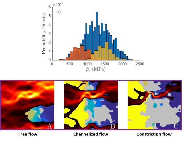
4.1. Qualitative Description

The permeability of a local-scale domain is described here through an example, depicted in Figure 5, extracted from the fractal topography. The comments we make are, however, general to all domains of both topographies studied. Moreover, the shape of the curve presented in Figure 5 has been observed in many theoretical observations [16,28,29,30,31] as well as experimental studies [1,32], considering both elastic and elasto-plastic materials.
The three flow situations depicted in Figure 5 represent three different regimes, which can also be identified in the graph plotting the permeability and the average pressure. At low loads, the free flow regime, depicted in Figure 5A, exhibits an (almost) free flow, close to the flow through non-contacting surfaces. In this regime, the separation of the surfaces is rather large and the contact is only held by a few asperities. This allows for a large permeability, but also makes the stiffness of the surfaces rather small, leading to a rapid decrease of permeability with increasing load. In order to describe the permeability in this regime one would be tempted to neglect the contact and follow Tripp [33] to obtain a close form for the permeability as a function of the average separation between the surfaces. Unfortunately, deformation cannot be neglected and this approach fails as soon as the surfaces enter in contact. Therefore, there is no available functional form to characterize this regime. As the applied pressure increases, the permeability enters in the channelized flow regime, in which permeability decays exponentially, which is reflected in Equation (3). As depicted in Figure 5B, the flow in this regime occurs only through few paths and the permeability decreases as these become narrower and eventually disappear. Eventually, see Figure 5C, most of the fluid pressure drops at a single location, identified as the critical constriction [16], thus entering in the constriction flow regime. As shown in Figure 5E and reflected in Equation (4), the permeability in this regime decreases following a power law, which, as identified by Dapp and Müser [34], is characteristic of saddle points.

4.2. Quantitative Description

In order to summarize the aforementioned behaviour in a quantitative manner, we fit a mathematical expression to it, shown in solid lines in Figure 5. When doing so, the free flow regime is ignored and the permeability of non-contacting surfaces is expressed as a simple function of the average separation, h ¯ . Of course, this introduces a significant error at low loads, but any static seal operating in the free flow regime has already failed and thus is not of interest in our study. The overall expression used to describe the permeability, K, thus reads
K = h ¯ 3 / 12 , p ¯ = 0 ,
K = e s p ¯ / p ¯ c + n , 0 < p ¯ < p ¯ T ,
K = c 2 1 p ¯ p ¯ c β , p ¯ T p ¯ < p ¯ c ,
K = 0 , p ¯ > p ¯ c ,
where n, s, c 2 , p ¯ T , β and p c are the fitting parameters, the interpretation of which can be given as follows: e n would be the permeability at zero load if the channelized flow regime would be extended to reach it; s is the slope in Figure 5D and thus indicates how rapidly the permeability decreases with increasing load in the channelized flow regime; c 2 would be the permeability at zero load if the constriction flow regime would be extended to reach it; p ¯ T marks the transition between the channelized and the constriction flow regimes and thus (approximately) marks the pressure above which all fluid pressure drops at a single constriction; β is the critical exponent governing the vanishing of permeability close to the percolation threshold and p ¯ c is the average pressure at the percolation threshold. In order to reduce the amount of fitting parameters, and to ensure a smooth description of the permeability, we demand continuity and derivablility at p ¯ = p ¯ T . This allows for expressing two parameters as a function of the others, i.e.,
p ¯ T = p ¯ c 1 β s ,
c 2 = e n β s β e β s .
Now, assuming that an estimate of s and n has been obtained by fitting the permeabilities at the channelized flow regime to Equation (3), permeability can be written, in the constriction flow regime, as
K = e s + n e β β s β 1 p ¯ p ¯ c β .
Thus, the following equation
log ( K ) ( s + n ) = β log 1 p ¯ p ¯ c + β 1 + log ( s ) log ( β )
can be used to fit β .
Of course, the thresholds between the three regimes are not known a priori and can vary significantly between different local-scale domains, as seen in Figure 4. Therefore, an algorithm is required to identify the different regimes and fit the parameters while keeping the number of average pressures at which permeability is computed low. Here, we present such an algorithm. To aid the presentation, we define the ordered list of points P i = p ¯ i , K i as the points computed up to a given current step. In addition, we define the groups G f , G e and G p as containing the points belonging to the free, channelized and constriction flow regimes and use I e and I p to mark the first and last points in G e . We then proceed as follows:
  • Find the average pressure, p ¯ c , at which the percolation threshold occurs: This is done by solving (only) the contact mechanics problem at increasing average contact pressures until a pressure at which there is no percolation is reached. Then, the value of p ¯ c is refined by means of a bisecting method.
  • Compute the permeability at three average pressures: These can be chosen freely, but we have observed that choosing them around 0.5 p ¯ c leads to a good performance.
  • Find the starting point of the channelized flow regime: Since the free flow regime is neglected, the starting point of the channelized flow regime is not a required parameter. However, it is imperative to ensure that all the points used to fit the parameters in Equation (3) do belong to the channelized flow regime. This is done in the following manner:
    3.1.
    Compute K p ¯ 0 .
    3.2.
    Form the groups G e = P 1 , G l = P 2 , P 3 , P 4 , G p = {} and set the index I e = 2
    3.3.
    Compute K p ¯ = ( p ¯ I e 1 + p ¯ I e ) / 2 and add the point to the list.
    3.4.
    Classify the computed points in the groups, using the following steps:
    • For every point, obtain s i , n i by fitting Equation (3) through the points P i 1 , P i and P i + 1 .
    • Find I s such that s I s is the smallest one.
    • For all points in the list, compute e r r i e = ( K i e x p ( s I s p ¯ i + n I s ) ) / K i .
    • Define I e as the index of the point with minimum load such that e r r i e < e r r 0 . If e r r I s 1 e > e r r 0 , assign I e = I s 1 instead.
    • Define I p as the index of the point with maximum load such that e r r i e < e r r 0 . If e r r I s + 1 l > e r r 0 , assign I p = I s + 1 instead.
    • Form the groups G f = P 1 , , P I e 1 , G e = P I e , , P I p , G p = P i | i > I p .
    3.5.
    If 2 ( p ¯ I e 1 p ¯ I e 1 ) / ( p ¯ I e 1 + p ¯ I e 1 ) < Δ p ¯ o b j , stop.
  • Populate the constriction flow regime, until it contains at least four points. For this, compute a point with a pressure between the maximum computed at the given step and p ¯ c . Then, update the group classification following 3.4.
Once this is done, the parameters n and s are fitted to Equation (3) using the points in G e and β is fitted to Equation (9) using the points in G p . The other two parameters, p ¯ T and c 2 , are then computed by means of Equations (6) and (7).
The error on the channelized flow regime is smaller than 5% in most of the domains studied. In a few domains, however, some points exhibit a larger error, up to 30%. This is caused by an inaccuracy in p ¯ T that leads to wrongly assign to the channelized flow regime points that belong to the constriction flow regime. This inaccuracy likely results from assuming a sharp transition between the regimes, whereas a small transition region can probably be expected to occur. In any case, less than 10% of the domains show this error. The error in the constriction flow regime is, however, larger, as it can go as high as 50%. Over 90% of the domains studied, however, show an error smaller than 20%. This larger error can be attributed to the discretization. Indeed, the size of critical constriction decreases as the percolation threshold is approached and thus a finer discretization becomes necessary. This can cause a deviation from the power law behaviour, as seen in Figure 5E. To avoid larger errors, β has been fitted without considering loads too close to p ¯ c whenever possible. As we shall present in Section 6, these errors, although not negligible, cause an error in the global-scale leakage smaller than the uncertainty in the results and thus can be considered acceptable.

5. A Stochastic Description of the Permeability at the Local Scale

Once the permeability of an individual local-scale domain is understood, the question arises as to how it varies between different domains extracted from the same topography. Figure 6 depicts this variability in terms of the parameters in Equations (3) and (4) as well as in terms of permeability at constant average pressure, expressed both in dimensions and dimensionless. For each parameter, three histograms are presented. One corresponds to the fractal topography, for which the values computed in the x- and y-direction have been blended due to the isotropy of the surface. The other two correspond to the turned surface, for which the values in each direction are presented separately.
Let us first pay attention to the permeability at a constant average pressure, p ¯ , depicted in Figure 6e for a high pressure and in Figure 6f for a low pressure. It is clearly apparent, especially at the higher pressure, that the permeability at a given constant p ¯ does not follow a log-normal distribution as utilized in [20]. This fact, caused by a bias against low permeabilities due to some domains being already beyond the percolation threshold, was already indicated in [15,35]. It is thus clear that, although the log-normal distribution could be used to describe permeability at low average pressures, this approach cannot be used in general. A promising alternative approach, which removes the aforementioned bias, is to use a log-normal distribution to describe the permeability at a constant reduced pressure, p ¯ / p ¯ c . As shown by the histograms depicted in Figure 6g,h, a log-normal distribution can indeed be used to describe the permeability at constant reduced pressures for all topographies. This approach has, however, a drawback, namely that both parameters describing the distribution will vary in a non-trivial manner with increasing load, making it harder to retrieve information from them.
A different, more fruitful approach is to study at the variation of the parameters in Equations (2)–(5). In particular, Figure 6a to d depict the histograms of p ¯ c , s, n and β , respectively. A Gaussian distribution seems appropriate to describe these histograms and we thus use it to model the uncertainty in the parameters. We notice, however, that other topographies may be better modelled by other distributions. Such a change should not affect the analysis presented in this work. It is interesting to discuss here how these histograms are expected to vary as the size of local-scale domains is increased. For this, we take β as an example. When studying this parameter in Gaussian topographies under elastic conditions, Dapp and Müser [30] found, in agreement with their previous theoretical work [34], a constant value for this parameter, namely, β = 3.45 . Given the similar behaviour, we observe in the constriction flow regime, we hypothesise that this should also hold for other types of surfaces and for plastically deformed ones. We also expect, however, that the lack of low-frequency cut-off as is the case in the local-scale domains studied here, should lead to a spread around β = 3.45 . The way in which this spreading occurs could, of course, depend on the particular topography studied. In our results, we notice that the value of β is centred quite close to β = 3.45 for all three cases (we have β ¯ = 3.83 , β ¯ = 3.79 and β ¯ = 3.28 for the fractal topography, the turned topography in x-direction and the turned topography in the y-direction, respectively), which gives credibility to our hypothesis. We can therefore expect that the probability density functions for β will tend to converge towards a delta function at β = 3.45 as the domain size increases the histogram. In fact, the same behaviour is to be expected for the other parameters, although the value at which they should converge is not known a priori. We finally point out that this convergence is the one that makes the classical homogenization possible when one can choose sufficiently large local-scale domains.

6. Global-Scale Leakage

In this section, a brief comment on the structure of the two-scale stochastic model is given. A flow chart of the model is presented in Appendix A. As seen by comparing with the flow chart corresponding to the model presented in [15,20] (see Appendix B), the main difference between the two lies in how we construct the global-scale permeability map and we should thus only focus on this part. To construct the permeabiltiy map, we use the Gaussian distributions describing the four parameters, p ¯ c , s, n and β . For every realization, a sample of each parameter is assigned to each global-scale point. From the global-scale contact mechanics model, the nominal pressure, p ¯ , is also known at these points for each load, W. Therefore, we can use Equations (2)–(5) to compute the permeability. Once this is known, leakage can be computed. This process is then repeated until a sufficient number of realizations has been carried out.
Let us now discuss the validity of the present approach. We start by noting that the deterministic model, presented in Section 2.1, has already been validated. Indeed, its two parts, i.e., the contact mechanics and the fluid flow model, are themselves widely used in the literature and have thus been validated several times. The reader is referred, for example, to the recent review by Vakis et al. [36], which discusses the applicability of the boundary element method to the contact of rough surfaces. Classical text books can be referred to concerning the use of Reynolds equation for the fluid flow model, e.g., [37]. For a direct validation of the coupling of the two parts of the deterministic model, in its application to leakage, the reader is referred to the work by Sahlin et al. [38] for a quantitative comparison with experiments and to [21] for a qualitative one. We also point out that similar assumptions have led Lorenz and Persson [28,39] to a model that compares well with experiments. We thus claim that we can trust the model developed in this work as long as it provides for the same answer as the deterministic model. Such a comparison is presented in Figure 7. It can be seen there that the deterministic solution falls inside the range of uncertainty provided by the two-scales solution, for sufficiently large loads. Of course, a much lower leakage is predicted at low loads, as the free flow regime was not considered. We can thus conclude that the stochastic two-scales model here presented is a valid tool for study of leakage through metal-to-metal seals.

7. Advantages of the Present Approach

Let us finish by discussing the advantages of the current model as compared with the previous ones. The advantage with respect to the model presented in [20] is clear, as it used a log-normal distribution to characterize the permeability at constant average pressure, which has been shown to be inaccurate. We thus focus the comparison with the model presented in [15].
The most obvious advantage is probably the gain in speed, which is of capital importance for the usability of the model, as it requires heavy computational power. To give a sense of this gain, the CPU time needed to compute the results for the fractal surface is given in Table 1 for the current model as well as for the model in [15]. The gain in time is clear there. Looking at it in more detail, we see that it includes both the computation of permeability at the local-scale domains and the computation of leakage at the global-scale domain, leaving only the meso-scale contact mechanics solution untouched. Concerning the local-scale permeability, the gain comes from the fact that it can be at fewer average pressures due to a more efficient representation of the power-law decay. Indeed, the large slope of the relation K ( p ¯ ) near the percolation threshold demands computing a lot of points there. Since the location of the percolation threshold is not known a priori, this affects the other regimes as well. By fitting a power-law decay at the constriction flow regime, the current model does not need to compute many points on this region. Similarly, few points are also needed in the other regimes. We can thus reduce the number of points to be computed around 47%. This leads to a reduction of CPU-time of about 39%. The gain in speed concerning the global-scale leakage computation comes from using Equations (2)–(5) to generate the permeability at the global-scale, instead of using interpolation. Since this part was the most costly in the global-scale flow solution in [15], a reduction of almost 100% in CPU-time can be achieved in this part. Since the computation of the permeabiltiy at the local-scale domains is, by far, the most costly part of the model, we can expect a total reduction time of almost 40%. We also notice that, when fitting the parameters, one has a clear idea on what error is committed by the finite number of local-scale domains assessed. Knowing this, one can set a criteria to avoid computing the permeability at too many local-scale domains.
Beyond the increased speed, the current model is more informative, which is an advantage in itself. Indeed, with the current model, one can easily pose questions such as: how does the spatial variation on the percolation threshold affect the global-scale performance of the seal? This would be much harder in a model where the permeability of local-scale domains is treated fully numerically. In addition, it becomes easier to correlate surface features with the final result, as one can first correlate the features with the parameters describing the local-scale permeability and then these with the global-scale performance.

8. Conclusions

In this work, we have first started by describing the permeability of local-scale domains. We have shown that three regimes can be identified, namely, a free, a channelized and a constriction flow regime. The three regimes present a different formulation for the relation between permeability and applied average pressure. This formulation can be described by means of four parameters, which vary randomly between different local-scale domains, following a Gaussian distribution. We have then used this description to enhance a stochastic two-scale model that had already been developed earlier. The new stochastic two-scale model has been tested against a deterministic solution, obtaining a good match in the prediction. In fact, the deterministic solution lays inside the range of possible stochastic solutions for sufficiently large loads. Finally, we have argued that the new model is faster, leading to a reduction in CPU-time of about 38%, and more informative in the interpretation of the results.

Author Contributions

Conceptualization, F.P.R. and A.A.; Methodology, F.P.R. and A.A.; Software, F.P.R. and A.A.; Validation, F.P.R. and A.A.; Formal Analysis, F.P.R. and A.A.; Investigation, F.P.R.; Resources, F.P.R. and A.A.; Data Curation, F.P.R.; Writing-Original Draft Preparation, F.P.R.; Writing-Review & Editing, F.P.R. and A.A.; Visualization, F.P.R.; Supervision, A.A.; Project Administration, A.A.; Funding Acquisition, A.A..

Funding

This research was founded by Shell Global International Solutions BV (Rijswijk, The Netherlands).

Acknowledgments

The authors are grateful to Shell Global International Solutions BV (Rijswijk, The Netherlands) for permission to publish and we wish to acknowledge both Shell Global Solutions International BV and the Swedish Research Council (VR) for financing this work.

Conflicts of Interest

The authors declare no conflict of interest.

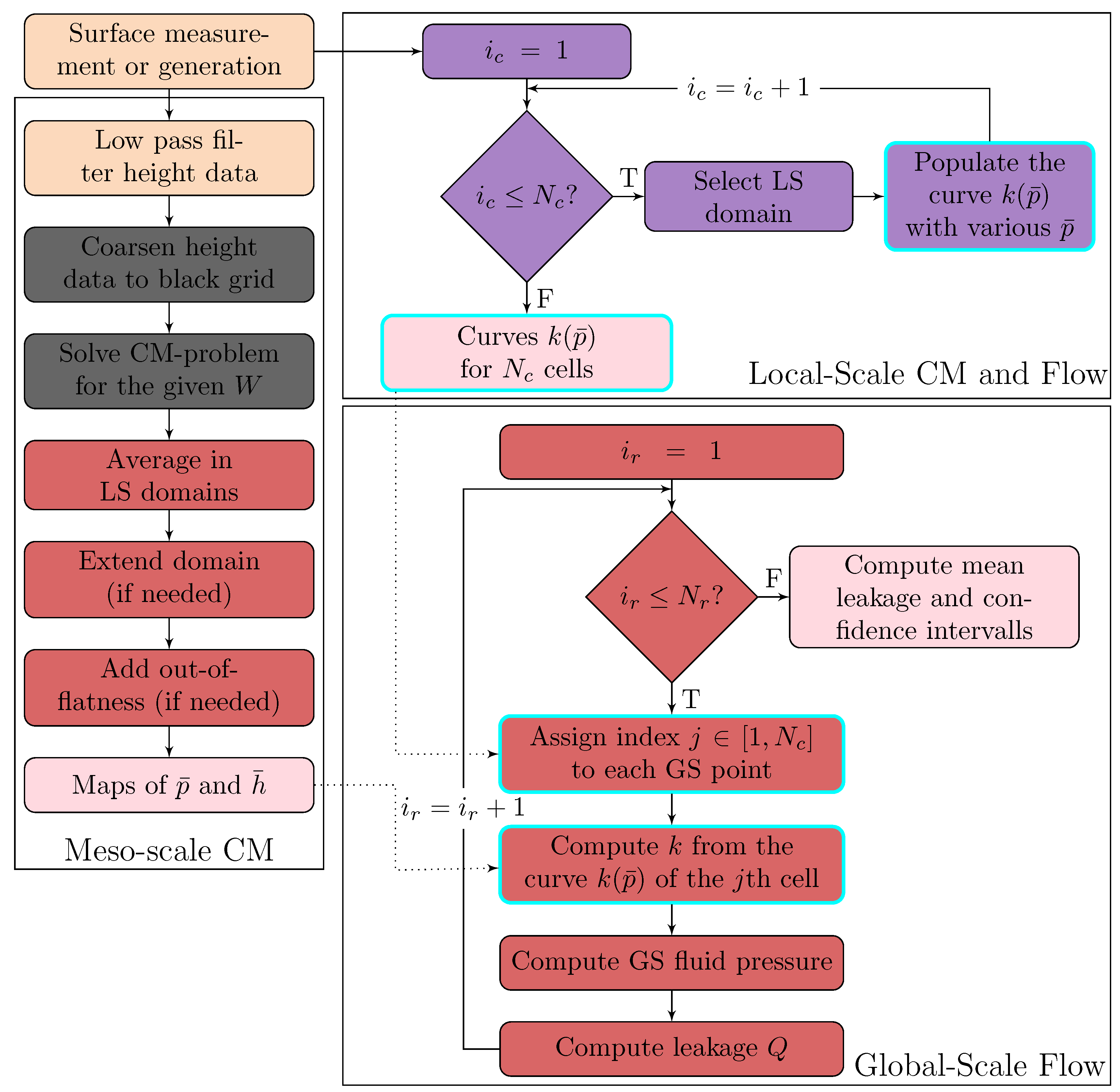
Appendix A. Flow Chart of the Model Presented in This Work

Figure A1. Flow chart for the numerical solution procedure of the stochastic two-scale model presented in this work. The pink boxes indicate middle or end results, and are connected by a dotted line to the box in the global-scale solver where they are used. The other colours indicate the grid or domain in which the operation is done, according to Figure 2, i.e., orange for the original grid, black for the meso-scale contact mechanics model, purple for the local-scale domain and red for the global-scale flow model. The boxes highlighted in blue are the ones changed with respect with the model presented in [15].
Lubricants 06 00087 g0a1

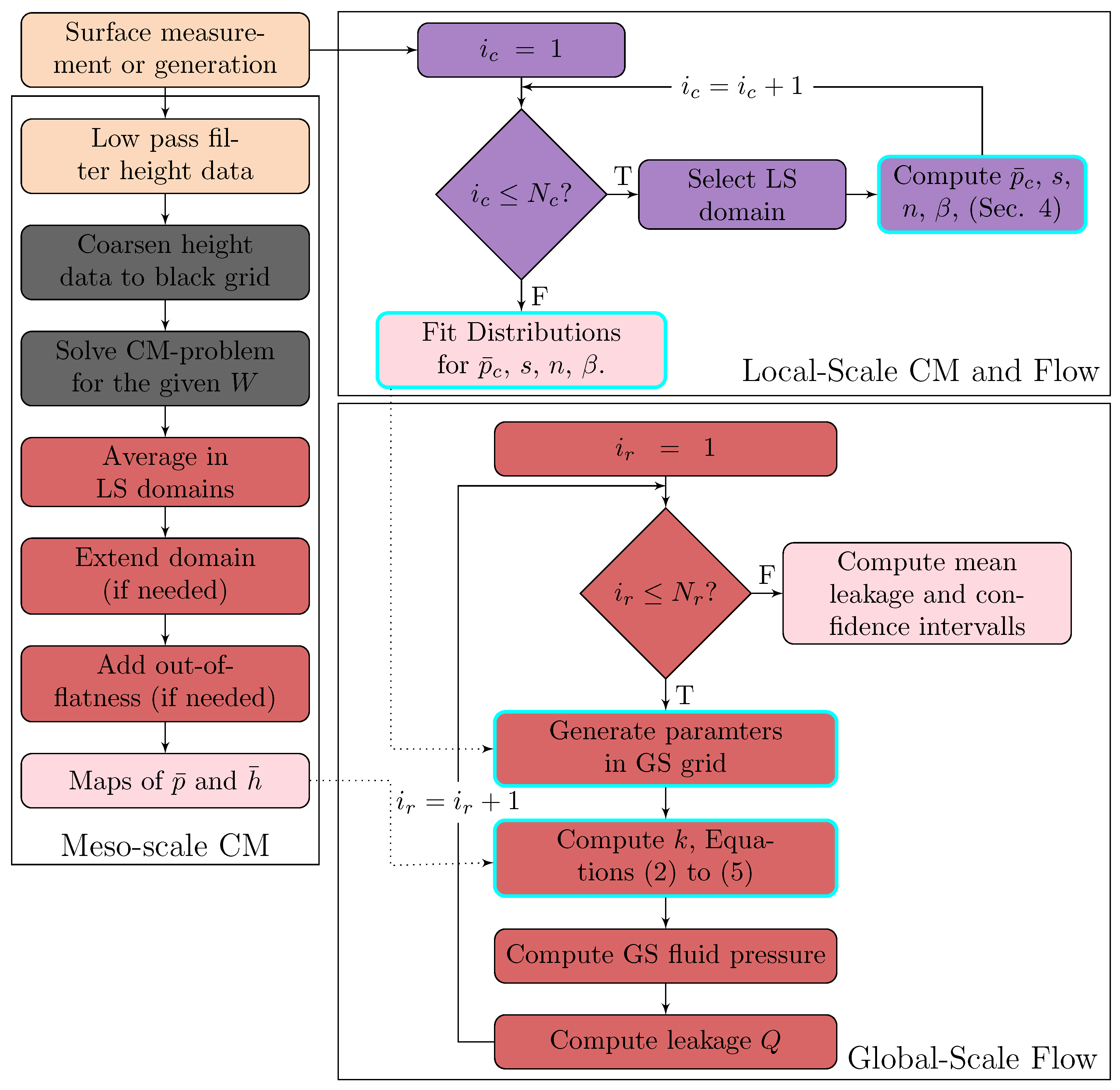
Appendix B. Flow Chart of the Model Presented the previous work

Figure A2. Flow chart for the numerical solution procedure of the stochastic two-scale model presented in [15]. The pink boxes indicate middle or end results, and are connected by a dotted line to the box in the global-scale solver where they are used. The other colours indicate the grid or domain in which the operation is done, according to Figure 2, i.e., orange for the original grid, black for the meso-scale contact mechanics model, purple for the local-scale domain and red for the global-scale flow model. The boxes highlighted in blue are the ones changed with respect to the model presented in this work.
Lubricants 06 00087 g0a2

References

  1. Marie, C.; Lasseux, D. Experimental leak-rate measurement through a static metal seal. J. Fluids Eng. 2006, 129, 799–805. [Google Scholar] [CrossRef]
  2. Geoffroy, S.; Prat, M. On the leak through a spiral-groove metallic static ring gasket. J. Fluids Eng. 2004, 126, 48–54. [Google Scholar] [CrossRef]
  3. Bollfrass, C.A. Sealing tubular connections. J. Pet. Technol. 1985, 37, 955–965. [Google Scholar] [CrossRef]
  4. Murtagian, G.R.; Fanelli, V.; Villasante, J.A.; Johnson, D.H.; Ernst, H.A. Sealability of stationary metal-to-metal seals. J. Tribol. 2004, 126, 591–596. [Google Scholar] [CrossRef]
  5. Hamilton, K.; Wagg, B.; Roth, T. Using ultrasonic techniques to accurately examine seal-surface-contact stress in premium connections. SPE Dril. Complet. 2009, 24, 696–704. [Google Scholar] [CrossRef]
  6. Inose, K.; Sugino, M.; Goto, K. Influence of grease on high-pressure gas tightness by metal-to-metal seals of premium threaded connections. Tribol. Online 2016, 11, 227–234. [Google Scholar] [CrossRef]
  7. Ernens, D.; de Rooij, M.B.; Pasaribu, H.R.; van Riet, E.J.; van Haaften, W.M.; Schipper, D.J. Mechanical characterization and single asperity scratch behaviour of dry zinc and manganese phosphate coatings. Tribol. Int. 2017, 118, 474–483. [Google Scholar] [CrossRef]
  8. Ernens, D.; van Riet, E.J.; de Rooij, M.B.; Pasaribu, H.R.; van Haaften, W.M.; Schipper, D.J. The role of phosphate conversion coatings in make-up and seal ability of casing connections. In Proceedings of the SPE/IADC Drilling Conference and Exhibition, The Hague, The Netherlands, 14–16 March 2018. [Google Scholar]
  9. Anwar, A.A.; Gorash, Y.; Dempster, W.; Hamilton, R. Literature research in relevant fields to understand pressure relief valve leak tightness in a static closed state. Procedia Eng. 2015, 130, 95–103. [Google Scholar] [CrossRef] [Green Version]
  10. Anwar, A.A.; Gorash, Y.; Dempster, W. Application of multi-scale approaches to the investigation of sealing surface deformation for the improvement of leak tightness in pressure relief valves. In Advanced Methods of Continuum Mechanics for Materials and Structures; Springer: Singapore, 2016; pp. 493–522. [Google Scholar]
  11. Zhang, B.; Hong, H.; Yu, M.; Yang, H. Leakage analysis and ground tests of knife edge indium seal to lunar sample return devices. Proc. Inst. Mech. Eng. Part G 2018. [Google Scholar] [CrossRef]
  12. Yan, Y.; Zhai, J.; Gao, P.; Han, Q. A multi-scale finite element contact model for seal and assembly of twin ferrule pipeline fittings. Tribol. Int. 2018, 125, 100–109. [Google Scholar] [CrossRef]
  13. Brunet, J.-C.; Poncet, A.; Trilhe, P. Leak-tightness assessment of demountable joints for the super fluid helium system of the cern large hadron collider (LHC). In Advances in Cryogenic Engineering; Springer US: Boston, MA, USA, 1994; pp. 657–662. [Google Scholar]
  14. Roman, A.; Ahmadi, G.; Issen, K.A.; Smith, D.H. Permeability of fractured media under confining pressure: A simplified model. Open Pet. Eng. J. 2012, 5, 36–41. [Google Scholar] [CrossRef]
  15. Pérrez-Ràfols, F.; Larsson, R.; van Riet, E.; Almqvist, A. On the loading and unloading of metal-to-metal seals: A two-scale stochastic approach. Proc. Inst. Mech. Eng. Part J 2018. [Google Scholar] [CrossRef]
  16. Persson, B.N.J.; Yang, C. Theory of the leak-rate of seals. J. Phys. Condens. Matter 2008, 20, 315011. [Google Scholar] [CrossRef]
  17. Lukkassen, D.; Nguetseng, G.; Wall, P. Two-scale convergence. Int. J. Pure Appl. Math. 2002, 2, 33–81. [Google Scholar]
  18. Sahlin, F.; Larsson, R.; Almqvist, A.; Lugt, P.M.; Marklund, P. A mixed lubrication model incorporating measured surface topography. part 1: Theory of flow factors. Proc. Inst. Mech. Eng. Part J 2010, 224, 335–351. [Google Scholar] [CrossRef]
  19. Scaraggi, M.; Carbone, G. A two-scale approach for lubricated soft-contact modeling: An application to lip-seal geometry. Adv. Tribol. 2012, 2012, 412190. [Google Scholar] [CrossRef]
  20. Pérez-Ràfols, F.; Larsson, R.; Lundström, S.; Wall, P.; Almqvist, A. A stochastic two-scale model for pressure-driven flow between rough surfaces. Proc. R. Soc. A 2016, 472, 20160069. [Google Scholar] [CrossRef] [PubMed] [Green Version]
  21. Pérez-Ràfols, F.; Larsson, R.; Almqvist, A. Modelling of leakage on metal-to-metal seals. Tribol. Int. 2016, 94, 421–427. [Google Scholar] [CrossRef]
  22. Reynolds, O. On the theory of lubrication and its application of Mr. Beauchamp tower’s experiments, including an experimental determination of the viscosity of olive oil. Philos. Trans. R. Soc. Lond. Ser. A 1886, 177, 157–234. [Google Scholar] [CrossRef]
  23. Pérez-Ràfols, F.; Wall, P.; Almqvist, A. On compressible and piezo-viscous flow in thin porous media. Proc. R. Soc. A 2018, 474, 2209. [Google Scholar] [CrossRef] [PubMed]
  24. Putignano, C.; Afferrante, L.; Carbone, G.; Demelio, G. A new efficient numerical method for contact mechanics of rough surfaces. Int. J. Solids Struct. 2012, 49, 338–343. [Google Scholar] [CrossRef]
  25. Nakamura, T.; Funabashi, K. Effects of directional properties of roughness and tangential force on pressure flow between contacting surfaces. Lubr. Sci. 1991, 4, 13–23. [Google Scholar] [CrossRef]
  26. Robbe-Valloire, F.; Prat, M. A model for face-turned surface microgeometry. application to the analysis of metallic static seals. Wear 2008, 264, 980–989. [Google Scholar] [CrossRef]
  27. Nitta, I.; Matsuzaki, Y.; Tsukiyama, Y.; Horita, M.; Sakamoto, S. Thorough observation of real contact area of copper gaskets using a laser microscope with a wide field of view. J. Tribol. 2013, 135, 041103. [Google Scholar] [CrossRef]
  28. Lorenz, B.; Persson, B.N.J.L. Leak rate of seals: Comparison of theory with experiment. EPL 2009, 86, 44006. [Google Scholar] [CrossRef] [Green Version]
  29. Dapp, W.B.; Lüke, A.; Persson, B.N.J.; Müser, M.H. Self-affine elastic contacts: Percolation and leakage. Phys. Rev. Lett. 2012, 108, 244301. [Google Scholar] [CrossRef] [PubMed]
  30. Dapp, W.B.; Müser, M.H. Fluid leakage near the percolation threshold. Sci. Rep. 2016, 6, 19513. [Google Scholar] [CrossRef] [PubMed] [Green Version]
  31. Persson, B.N.J. Leakage of metallic seals: Role of plastic deformations. Tribol. Lett. 2016, 63, 42. [Google Scholar] [CrossRef]
  32. Zhang, F.; Liu, J.; Ding, X.; Yang, Z. An approach to calculate leak channels and leak rates between metallic sealing surfaces. J. Tribol. 2017, 139, 011708. [Google Scholar] [CrossRef]
  33. Tripp, J.H. Surface roughness effects in hydrodynamic lubrication: The flow factor method. J. Lubr. Technol. 1983, 105, 458–463. [Google Scholar] [CrossRef]
  34. Dapp, W.B.; Müser, M.H. Contact mechanics of and reynolds flow through saddle points: On the coalescence of contact patches and the leakage rate through near-critical constrictions. EPL 2015, 109, 44001. [Google Scholar] [CrossRef]
  35. Waseem, A.; Guilleminot, J.; Temizer, I. Stochastic multiscale analysis in hydrodynamic lubrication. Int. J. Numer. Methods Eng. 2017, 112, 1070–1093. [Google Scholar] [CrossRef]
  36. Vakis, A.I.; Yastrebov, V.A.; Scheibert, J.; Nicola, L.; Dini, D.; Minfray, C.; Almqvist, A.; Paggi, M.; Lee, S.; Limbert, G.; et al. Modeling and simulation in tribology across scales: An overview. Tribol. Int. 2018, 125, 169–199. [Google Scholar] [CrossRef]
  37. Hamrock, B.J. Fundamentals of Fluid Film Lubrication; McGraw-Hill, Inc.: New York, NY, USA, 1994. [Google Scholar]
  38. Sahlin, F.; Larsson, R.; Marklund, P.; Almqvist, A.; Lugt, P.M. A mixed lubrication model incorporating measured surface topography. part 2: Roughness treatment, model validation, and simulation. Proc. Inst. Mech. Eng. Part J 2010, 224, 353–365. [Google Scholar] [CrossRef]
  39. Lorenz, B.; Persson, B.N.J. Leak rate of seals: Effective-medium theory and comparison with experiment. Eur. Phys. J. E 2010, 31, 159–167. [Google Scholar] [CrossRef] [PubMed] [Green Version]
Figure 1. A schematic representation of the two-scale model, including the fluid flow (left) and contact mechanics (right) parts. On the left, the red arrows represent the direction and magnitude of the (global-scale) fluid flow, while the yellow to blue colormap depicts the (global-scale) fluid pressure. The insert reflects that each arrow summarizes a detailed, local-scale flow pattern. On it, the pattern coloured in red reflects the (local-scale) flow while the (local-scale) fluid pressure is depicted by a yellow to blue colormap. On the right, the average contact pressure p ¯ is depicted. Again, the insert reflects that each global-scale point hides a detailed local-scale contact pressure distribution. This figure has been adapted from [15].
Lubricants 06 00087 g001
Figure 2. Representation of the three grids used in the two-scale model. In orange, the finest grid, with which the smaller details are captured. The red dots represent the global-scale grid between whose points the global-scale flow, j, depicted by red arrows, is computed. The intermediate black grid is used in the global-scale contact mechanics model. Two local-scale domains where permeability is computed are depicted in purple and green. This figure has been adapted from [15].
Lubricants 06 00087 g002
Figure 3. The two initial gaps used in this work. On the (top), corresponding to a (generated) self-affine fractal surface. On the (bottom), corresponding to a (measured) turned surface. The superimposed grid depicts the local-scale domains used to compute the permeability. This figure has been adapted from [15].
Lubricants 06 00087 g003
Figure 4. Permeability, K, as a function of the applied average pressure, p ¯ , corresponding to the two topographies studied. In (a), the same data is presented as in (b), but in non-dimensional form. The average pressure is scaled by the average pressure at the percolation threshold p ¯ c . Regarding the scaling factor for the permeability, e n , the reader is referred to Equation (3).
Lubricants 06 00087 g004
Figure 5. On top, the three flow regimes are depicted, i.e., (A) the free-flow regime, (B) the channelized flow regime and (C) the constriction flow regime, the corresponding pressure points of which are marked on the bottom figures by the black diamond. These three sub-figures should be interpreted as follows: the situation represented corresponds to the flow through the gap left when a rough surface is pressed against a flat one at different average pressures, indicated in the bottom sub-figures. The area where the surfaces are in contact is marked in grey. The fluid flow is marked in a reddish colour scale (yellow meaning high flow and black meaning almost no flow). Finally, wherever the flow is small, the fluid pressure has been superimposed in a colour scale from yellow (high inlet pressure) to blue (low, outlet pressure). On the bottom (D,E), the permeability as a function of the reduced average contact pressure, using different axes. The blue dots mark the permeability as computed at regular pressure intervals while the red dots mark the points calculated using the algorithm presented in Section 4.2. The solid lines correspond to the fitting given by Equations (3) and (4). The vertical dashed lines mark the transition between the different regimes. The black dot deviating from the power-law on the right line is the result of an insufficient discretization, depicted only for illustrative purposes.
Lubricants 06 00087 g005
Figure 6. Summary of the stochastic behaviour of permeability of local-scale domains. (ad) depict the histogram for the parameters in Equations (3) and (4), p ¯ c , s, n and β ; (e,f) depict the permeability (in logarithmic scale) at a constant average pressure, p ¯ . Finally (g,h) depict the permeability (in logarithmic scale) at a constant reduced average pressure, p ¯ / p ¯ c . The probability density of the fractal surfaces include both x and y-directions and has been doubled for visualization processes.
Lubricants 06 00087 g006
Figure 7. Comparison between the deterministic model in [15] (red marks) and the current stochastic, two-scales model (blue lines). The solid line depicts the mean value of the different realizations performed while the dashed lines mark the 95% confidence interval. The comparison corresponding to the fractal (turned) topography is depicted on the left (right).
Lubricants 06 00087 g007
Table 1. Comparison of CPU time needed to obtain a full solution as in Figure 7, corresponding to the fractal surface. LS, MS and GS stand for local-, meso- and global-scale, respectively. The average time per domain of the local-scale pemreabiltiy has been computed using 72 domains. The times for the MS Contact Mechanics model and the GS flow model correspond to the loads in Figure 7. The total time includes 72 local-scale domains.
LS Permeability
(Average Time Per Domain)
MS Contact MechanicsGS FlowTotal
Algorithm in [15]7986 s3301 s4406 s162 h
New algorithm4904 s3301 s11 s99 h
Difference 39 % 99 % 0 % 39 %

