On Monitoring Physical and Chemical Degradation and Life Estimation Models for Lubricating Greases

Abstract

Degradation mechanisms for lubricating grease are categorized and described. An extensive survey of the available empirical and analytical grease life estimation models including degradation monitoring standards and methods are presented. A summary of the important contributions on grease degradation is presented.

1. Introduction

The lubricating effectiveness of grease is limited by both physical and chemical deteriorations caused by shear stresses, pressure, and the severity of operating conditions, particularly temperature. Degraded grease becomes inefficient and eventually loses its lubrication capacity such that it can adversely affect the machine’s performance and functionality. Proper monitoring of degradation and on-schedule replacement/replenishment of grease are important facets of machinery maintenance practices. Presently, grease replacement is performed periodically according to time schedules adapted from empirical models. Although some empirical relationships for estimating grease life are available, they tend to be restrictive. The drawback of empirical models is limited applicability when the working condition of grease is different from the operating conditions from which the empirical models were derived. In applications where the bearing element is lubricated and sealed for life, there are quality control standard procedures to measure the grease resistance to different degradation processes.

The earliest reviews of grease lubrication research appeared some 50 years ago from Barnett [1] and Langborne [2], who summarized the American and British publications, respectively. In 1997, Rush [3] wrote a review of the more common standard grease tests. More recently, Lugt [4] presented a very useful summary on grease lubrication in rolling bearings. He also published a comprehensive book [5] on the subject of grease lubrication.

This paper presents a review of published works and the authors’ perspective on the present empirical and analytical grease life estimation models, including popular grease degradation monitoring methods and a summary of the pertinent contributions on this subject matter, based on the information available in the literature.

The published papers are categorized based on different grease degradation mechanisms including mechanical, chemical, base oil evaporation/separation, and contamination. A summary table of all related literature is presented at the end of this paper.

2. Empirical Models

Most empirical models for predicting grease life (replenishment time) are developed by bearing manufacturers [4]. They are normally presented in manufacturers’ catalogues using a specific bearing size, speed, and working temperature. Booser [6] presented a model for estimating grease life by considering the most influential factors such as temperature, grease composition, bearing speed, and load. For the effect of temperature, he reported the following empirical logarithmic–reciprocal absolute temperature relation, inspired by the Arrhenius equation:

$$Log L_0=K_G+\frac{K_T}{273+T},$$

(1)

where $L_0$ is the geometric mean grease life without accounting for either speed or load. $K_T=2450$ is the temperature factor developed based on observations that the grease life drops by a factor of 1.5 for each 10 °C temperature rise. $K_G$ is the life parameter, which depends on the composition of the grease. Comparing the values of $K_G$ for different greases, Booser chose a typical value of $K_G=-2.30$.

To implement the effect of speed on grease life reduction, Booser included two additional terms in Equation (1) in terms of a half-life subtraction speed factor $S_G$ (tabulated for different greases) and a $DN$ factor, as shown below:

$$Log L_0=-2.30+\frac{2450}{273+T}-0.301 S_G-0.26 \frac{DN}{{\left(DN\right)}_L},$$

(2)

where $D$ is the shaft diameter at bearing seat in millimeter, $N$ is speed in rpm, and ${\left(DN\right)}_L$ is the limiting $DN$ value for different ball bearing types (approximately 270,000 for medium cross section ball bearings).

Also, to account for effect of load, Booser incorporated an additional term as follows:

$$Log L_0=-2.30+\frac{2450}{273+T}-0.301 S_G-0.26 \frac{DN}{{\left(DN\right)}_L}-0.18 \frac{NDW}{C^2},$$

(3)

where $W$ is the radial load and $C$ is the specific dynamic capacity of the ball bearing ($W$ and $C$ are in pounds).

To simplify Equation (3), Booser went on to define a total half-life subtraction speed factor $S=S_G+S_N+S_W$ where:

$$S_N=0.864 \raisebox{1ex}{$DN$}\!\left/ \!\raisebox{-1ex}{${\left(DN\right)}_L$}\right.$$

$$S_w=0.61 \raisebox{1ex}{$NDW$}\!\left/ \!\raisebox{-1ex}{$C^2$}\right..$$

This simplified Equation (3) to:

$$Log L_0=-2.30+\frac{2450}{273+T}-0.301 S.$$

(4)

Similarly, by considering the effect of temperature, speed, and load on the life of grease, Kawamura et al. [7] also presented two grease life formulas for Urea and lithium soap greases.

Emphasizing the effect of temperature, Booser and Khonsari [8] studied the grease life in different temperature zones. In their model, the life of grease in different temperatures is extrapolated from stable conditions. In high temperatures (above 160 °C) where the grease life is limited by oxidation, they suggested using an Arrhenius equation in the form of:

$$Log L=A+\frac{B}{273+T},$$

(5)

where $A$ and $B$ are constants. Assuming that the grease life drops in half for a 10 °C rise in this temperature zone, $B$ is calculated to be 6000 and $A=10.75$.

For lower temperatures between 70 and 160 °C (warm zone), they assumed that the grease life drops by a factor of 1.5 per 10 °C temperature rise because of base oil evaporation. Their presented formula for predicting the life of grease in the warm zone is very close to Equation (1) presented earlier by Booser:

$$Log L=D+\frac{E}{273+T},$$

(6)

where E = 2450 and D = −2.6.

For normal industrial temperature zone, they suggest using the bearing manufacturer re-lubrication life period of 40,000 h.

In low temperatures (below 40 °C), considering the effects of grease hardening and high oil viscosity, they estimated the grease life from its life at 40 °C using the change in its base oil viscosity $\nu$:

$$L=L_{40 °\mathrm{C}} \times {(\raisebox{1ex}{$\nu $}\!\left/ \!\raisebox{-1ex}{${\nu }_{40}$}\right.)}^2.$$

(7)

The calculated grease life from Equations (5) to (7) needs to be modified by adding correction factors for demanding conditions of high DN operation, centrifugal grease throw-off, outer ring rotation, and cage effect as described in their paper. Figure 1 shows guidelines for bearing re-greasing intervals with mild operating conditions adapted from [9].

3. Lubricant Degradation Processes

Grease degradation is categorized into physical and chemical degradation [5,11]. Physical degradation covers all the physical changes in the grease during usage. This degradation category includes the integral parts of mechanical degradation (breaking of grease thickener’s structure), increased base oil separation, base oil evaporation, and also increased contamination. Chemical degradation covers all the chemical reactions inside the grease that affect grease lubricating life including additive depletion (mostly antioxidant), base oil oxidation, and thickener oxidation. Physical degradation is more sensitive to applied force (shear stress) and velocity (shear rate), and chemical degradation is more sensitive to operating temperature.

3.1. Mechanical Degradation

Lubricating grease consists of a lubricant base oil (liquid) and a thickener agent that keeps the base oil. There are different types of base oil and thickeners, but normally the thickener is a long fiber structure with aggregated molecules. Figure 2 shows a SEM image of the thickener structure of a fresh lithium-complex grease. The image is obtained after washing out the base oil using a volatile solvent.

When a grease experiences mechanical shear/force, the structure of its thickener breaks down mechanically. This is a gradual process called grease mechanical degradation. Mechanical degradation is an irreversible process associated to the permanent changes in the grease structure (Recoverable, temporary changes in the grease structure are not considered to be mechanical degradation). Mechanical degradation is the most dominant degradation process in low and medium operating temperatures (between 40 °C and 70 °C). This range of operating temperature covers many bearings in electro-motors as well as a wide variety of other industrial applications. In addition, at lower temperatures (below 40 °C), the grease degradation can be considered to be mechanically dominated [8]. Figure 3 shows the broken structure (with shorter and thinner fibers) of the same grease after 15 h of shearing in a rheometer with a shear rate of 5000 1/s in 25 °C.

After breaking the thickener structure, the grease loses its consistency and becomes softer. However, since the broken structure is not able to retain the base oil, the bleeding rate of the grease increases, and as a result the grease becomes dry and hard. Increasing the load and speed accelerates the mechanical degradation. Generally, low temperature can also make the grease harder and more prone to mechanical breakdown. A bearing element suffers from starvation in low temperatures more than mechanical degradation because of limited grease mobility. Khonsari and Booser [8] showed empirically that grease experiences a distinctive drop in life in temperatures lower than 40 °C, which is proportional to the square of the base oil viscosity changes.

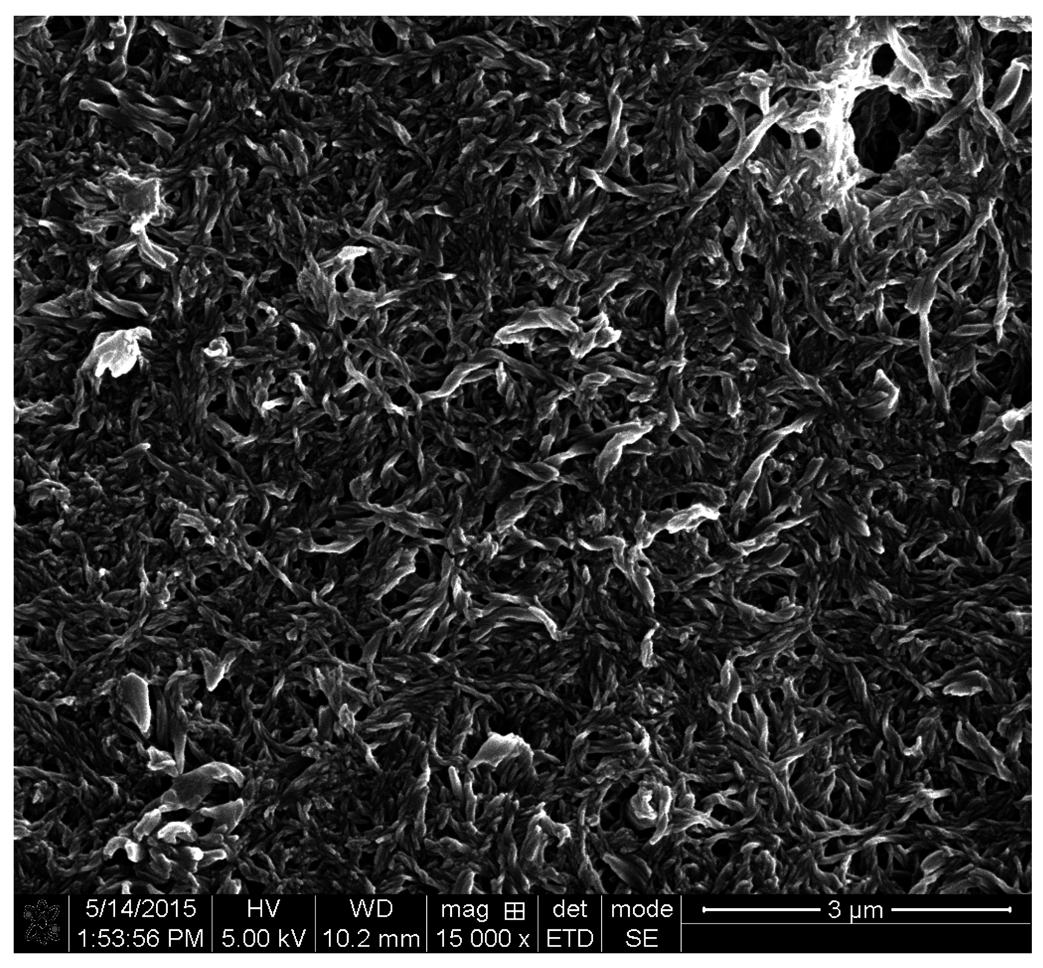
3.1.1. Mechanical Degradation Monitoring

There are several methods to monitor mechanical degradation. Scanning electron microscopy can be used to examine the structure of a grease before and after degradation, but it is difficult to measure the degradation quantitatively by this method. The grease sample also should be prepared by washing the base oil with a solvent.

Standard Test Methods for Cone Penetration of Lubricating Grease (ASTM D217) is a popular method to measure grease consistency and can be used as a measure of the grease mechanical degradation. Based on the standard method, fresh grease should be worked by a grease worker before penetration test. The penetration measured by a rheometer has also been used in [12] as a mechanical degradation monitoring parameter.

An important parameter for characterizing the behavior of grease is the shear stress. Monitoring the variation of shear stress as a function of time in a constant shear rate reveals how grease softens. Figure 4 shows a typical shear stress curve of worked XHP 222 grease when it is sheared in a rheometer with a constant shear rate of 2500 1/s and at a constant temperature of 35 °C [13].

The shear stress decreases until it reaches its minimum value at $\tau (\infty )$. Different empirical shear stress functions have been presented by researchers [14,15,16]. In a recent paper [13], the correlation between mechanical degradation and entropy generation introduced in [12] was used to generate an analytical shear stress function. Some of these models are presented in the sections that follow.

3.1.2. Mechanical Life Estimation Models

Mechanical degradation is an irreversible process. The mechanical energy is dissipated inside the grease, breaks the structure of the thickener, and generates heat. Since the whole process involves energy transfer and entropy generation, it can be studied from an energy/entropy point of view.

Kuhn developed a model for characterizing the grease mechanical degradation from an energy point of view. By analogy to the solid body wear, he defined an apparent rheological energy density $e_{Rrheo}^{*}$ that is the sustainable energy level per volume unit of grease for a certain level of structural degradation. This energy is dissipated by frictional force between the layers of the grease during a shearing process [17]. In a viscometric flow with a controlled shear stress of $\tau ={\tau }_c=\mathrm{constant}$, he calculated the energy density simply from the product of the shear stress and the strain rate as follows [18]:

$$e_{rh}\left(t\right)={\tau }_c{{\displaystyle \int }}_0^t\dot{{\rm Y}}\left(\xi \right)d\xi .$$

(8)

In a controlled shear strain (rate) test with a shear rate of ${\rm Y}={{\rm Y}}_c=\mathrm{constant}$, Kuhn calculated the energy density as follows [18]:

$$e_{rh}\left(t\right)={\dot{{\rm Y}}}_c{{\displaystyle \int }}_0^t\tau \left(\xi \right)d\xi .$$

(9)

He used Equations (8) and (9) to calculate $e_{Rrheo}^{*}$.

Kuhn then introduced the following empirical model for shear stress as a function of time [14,19]:

$$\tau \left(t\right)={\tau }_{lim}·{(\frac{t}{t_{lim}})}^{-n} \left[\mathrm{pa}\right],$$

(10)

where ${\tau }_{lim}$ is defined as the final nearly constant value of shear stress versus stress time. Since at t = 0 this equation returns a zero value for initial shear stress, he stated that the equation is not defined at t = 0.

Using Equation (9), Kuhn then estimated the energy that is necessary to obtain a limiting shear stress [14,19]:

$$e\left(t\right)={\tau }_{lim}·\left(\frac{1}{-n+1}\right)·{(\frac{t}{t_{lim}})}^{\left(-n+1\right)} [\frac{J}{{\mathrm{mm}}^3}].$$

(11)

Utilizing this concept, he defined a mechanical dissipation function to characterize the structural degradation of grease. Further, considering the irreversibility of the mechanical degradation, Kuhn suggested the application of thermodynamic entropy in the study of mechanical degradation of lubricating grease [20,21].

Applying the thermodynamic entropy concept, Rezasoltani and Khonsari [12] developed a correlation between mechanical degradation and energy accumulation/entropy generation inside the grease. The correlation was validated experimentally using three different test rigs. They monitored grease consistency as a measure of mechanical degradation during prolonged shear processes at different shear rates and temperatures (up to 45 °C) and showed that in the normal industrial temperatures where the mechanical degradation is the dominant degrading process, mechanical degradation depends only on the generated irreversible entropy inside the grease regardless of test conditions (shear rate and temperature). The correlation was used to establish a grease mechanical life prediction model published in their recent paper [13]. The model is capable of predicting the reduction in the grease consistency as a result of mechanical degradation. The end of grease mechanical life is defined when the grease consistency is reduced to a minimum acceptable value beyond which the grease may leak out from the bearing under centrifugal forces or becomes ineffective because of oil loss after excessive oil bleeding/separation. An appropriate minimum acceptable consistency must be defined for a specific application considering the costs and safety factors. The model predicts the length of time to reach the minimum acceptable consistency, which signals when the grease needs to be replenished.

The grease mechanical degradation is non-uniform and very much depends on the location of the grease inside the bearing. In other words, grease directly located within an EHL contact, for example, degrades much faster than grease accumulated on either side of the contact, where shear rate and stresses are much lower. Therefore a good understanding of grease flow and the stresses experienced by the grease in critical locations inside the bearing is essential prior to applying the mechanical life estimating models.

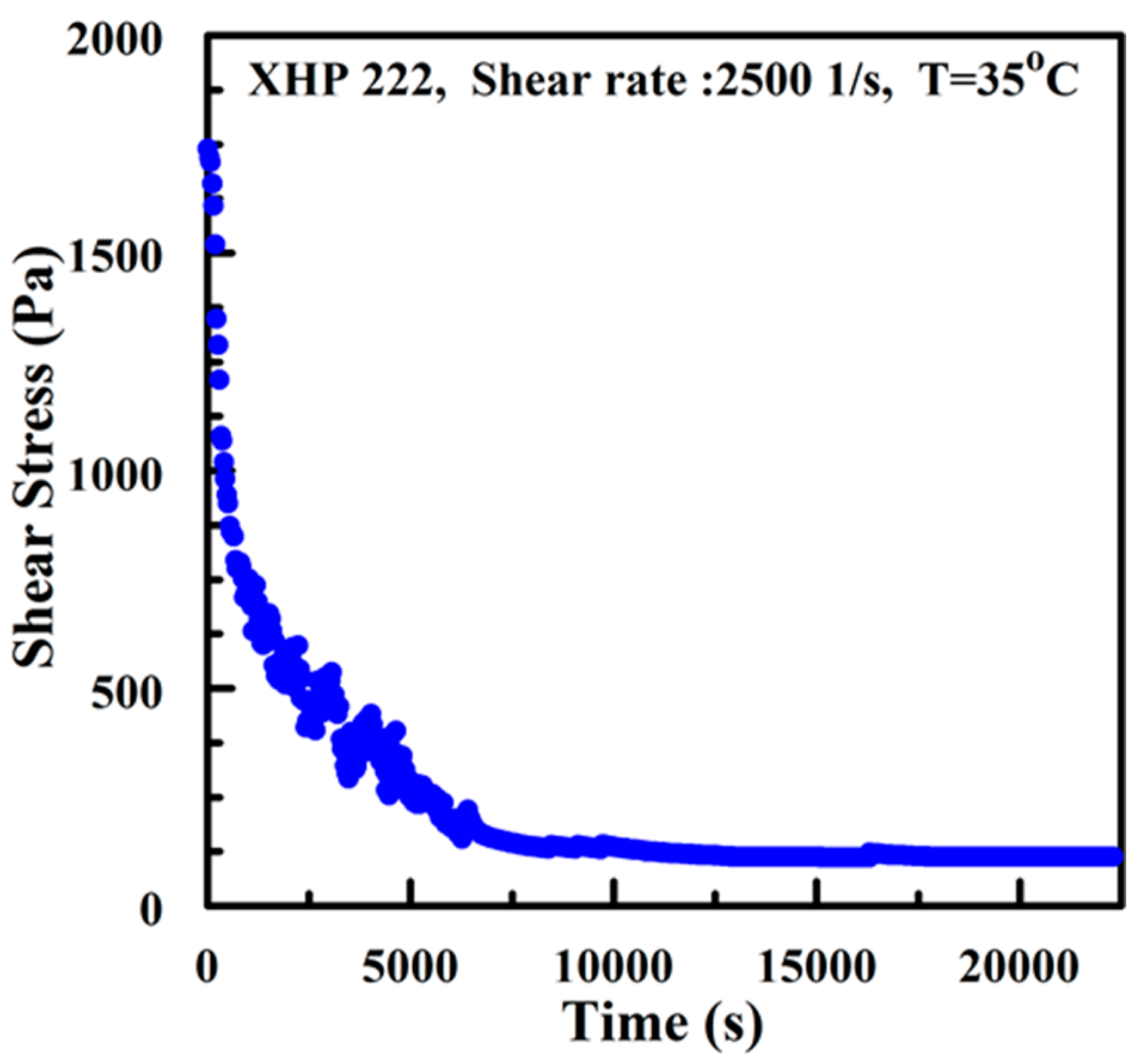
3.1.3. Shear Stress Empirical Functions

There are several empirical models for modeling the shear stress of grease as a function of time. Some of them—the Kuhn model [14], the Czarny model [16], and the Bauer model [15]—are reported here by Equations (12)–(14), respectively:

$$\tau \left(t\right)={\tau }_{\infty }·{\left(\frac{t}{t_{lim}}\right)}^{-n}$$

(12)

$$\tau \left(t\right)={\tau }_{\infty }+c·t^m$$

(13)

$$\tau \left(t\right)={[k_1·\left(m-1\right)·t·{{\tau }_0}^{1-m}+{\left({\tau }_0-{\tau }_{\infty }\right)}^{1-m}]}^{\frac{1}{1-m}}+{\tau }_{\infty }.$$

(14)

In the above models, ${\tau }_0$ is the initial shear stress value at time zero, and ${\tau }_{\infty }$ is the final constant shear stress reached at $t_{\infty }$ or $t_{lim}$. Other parameters (n, m, …) are constants unique to the grease and must be determined experimentally.

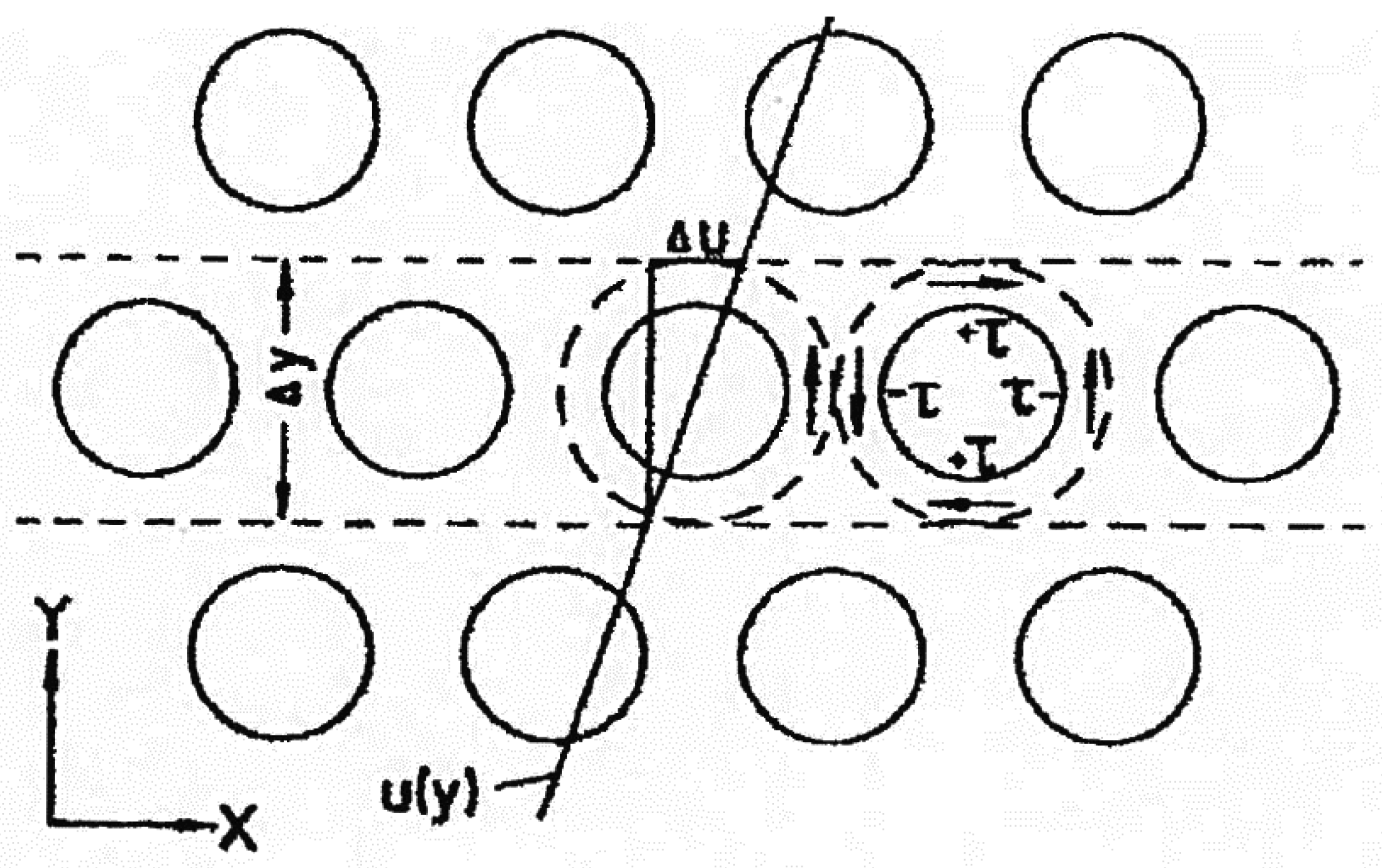
3.1.4. Shear Stress Analytical Functions

Spiegel et al. [22] studied the grease softening analytically. They assumed that grease consists of large particles that, upon applying a shearing action, tend to break down into smaller spherical particles. They assumed that during revolution each particle is subjected to surface shear twice by its neighboring particles (once in the direction of rotation and once in the opposite direction; see Figure 5).

Spiegel et al. further assumed that the particle size decreases gradually as a result of the shearing action and that the reduction in particle size will continue until it reaches a final value. They concluded that since it is easier to roll the smaller size particles, the grease becomes softer (loses consistency) by particle size reduction. They went on to define Z as the number of load cycles (rotation of the particles). They related the angular velocity ω and frequency of rotation $f$ of the particles to the shear rate in a shearing action:

$$\dot{{\rm Y}}=\frac{\omega }{2}=\left(\pi ·f\right).$$

(15)

Based on their definition of Z, the frequency of rotation $f$ is equal to the number of load cycles Z. Then, for a shearing action with the shear rate of $\dot{\gamma }\left(t\right)$ from $t=t_b$ to $t=t_e$, they wrote:

$$Z=\frac{1}{\pi }{{\displaystyle \int }}_{t_b}^{t_e}\dot{\gamma }\left(t\right)dt.$$

(16)

For a constant shear rate,

$$Z=\frac{\dot{\gamma }\left(t_e-t_b\right)}{\pi }.$$

(17)

They also assumed a Wohler curve between shear stress and Z:

$$\ln \tau \left(t\right)=f\left(\ln \left(Z\right)\right)$$

(18)

and finally came up with the following equation for calculating the decrease in shear stress:

$$\tau \left(t\right)={\tau }_{\infty }+\left({\tau }_0-{\tau }_{\infty }\right)·e^{\frac{z}{z_0}},$$

(19)

where $Z_0$ is a reference number of load cycles, ${\tau }_{\infty }$ is the yield stress when Z → ∞, and ${\tau }_0$ is the yield stress for Z = 0. The number of load cycles Z is calculated differently from shear rate for each application. For example, for the standard grease worker (DIN ISO 2137) it is defined as:

$$z=\frac{8·\varnothing · {(\frac{D_m}{d})}^2·H}{\pi ·d ·i},$$

(20)

where $D_m$ is the diameter of the grease worker plunger disc (0.075 m), d is the diameter of the holes on the disc (0.00635 m), H is the height of the chamber (0.0635 m), $i$ is the number of holes on the disc (51 holes), and $\varnothing$ is a number that defines the non-Newtonian behavior (for Newtonian behavior $\varnothing$ = 1).

For the grease flow inside a pipe with length L and diameter D they defined:

$$z=\frac{8 L}{\pi ·D}.$$

(21)

Although the model developed by Spiegel et al. is based on several assumptions (such as a spherically shaped thickener’s particles and a particle’s size reduction mechanism), it predicted the reduction in the shear stress well. Their model can be used for comparing grease mechanical life in different applications such as flow in a pipe versus grease worker, but cannot be used as a general model for grease mechanical life prediction.

A more comprehensive shear stress function was derived by Rezasoltani and Khonsari [13]. Considering a shear process with a shear rate of $\dot{\gamma }\left(t\right)$, they define ${\tau }^{*}\left(t\right)=\tau \left(t\right)-\tau (\infty )$, where $\tau \left(t\right)$ denotes the shear stress at time t. Then they express the shear stress at time t + dt as:

$${\tau }^{*}\left(t+dt\right)={\tau }^{*}\left(t\right)-\alpha ·d{S}_g,$$

(22)

where $d{S}_g=\frac{{\mathsf{\tau }}^{*}\left(t\right)·\dot{\gamma }\left(t\right)}{T\left(t\right)}dt$ is the generated entropy during the small time increment of dt, and $\alpha$ is assumed to be a unique parameter for grease at the testing conditions.

$${\mathsf{\tau }}^{*}\left(t+dt\right)={\mathsf{\tau }}^{*}\left(t\right)-\alpha ·\frac{{\mathsf{\tau }}^{*}\left(t\right)·\dot{\gamma }\left(t\right)}{T\left(t\right)}dt$$

(23)

After replacing $\frac{{\mathsf{\tau }}^{*}\left(t+dt\right)-{\mathsf{\tau }}^{*}\left(t\right)}{dt}$ by $\dot{{\mathsf{\tau }}^{*}}\left(t\right)$ which is equal to $\dot{\tau }\left(t\right)$, one arrives at the following:

$$\dot{\tau }\left(t\right)+\frac{\alpha ·\dot{\gamma }\left(t\right)}{T\left(t\right)}·{\mathsf{\tau }}^{*}\left(t\right)=0$$

(24)

$$\dot{\tau }\left(t\right)+\frac{\alpha ·\dot{\gamma }\left(t\right)}{T\left(t\right)}·\mathsf{\tau }\left(t\right)=\frac{\alpha ·\dot{\gamma }\left(t\right)}{T\left(t\right)}·\mathsf{\tau }(\infty )$$

(25)

$$\dot{\tau }\left(t\right)+\frac{\alpha ·\dot{\gamma }\left(t\right)}{T\left(t\right)}·\tau \left(t\right)=\beta \left(t\right),$$

(26)

where $\beta \left(t\right)=\frac{\alpha ·\dot{\gamma }\left(t\right)}{T\left(t\right)}.\tau (\infty )$.

Equation (26) (a first-order, linear ordinary differential equation (ODE)) has a solution in the form of:

$$\mathsf{\tau }\left(t\right)=e^{-{\displaystyle \int }\frac{\alpha ·\dot{\gamma }\left(t\right)}{T\left(t\right)}dt}({\displaystyle \int }\beta \left(t\right)·e^{{\displaystyle \int }\frac{\alpha ·\dot{\gamma }\left(t\right)}{T\left(t\right)}dt}dt+C),$$

(27)

where τ(t), $\dot{\gamma }\left(t\right)$, T(t) are shear stress, shear rate, and temperature as functions of time, respectively. $\dot{\gamma }\left(t\right)$ and T(t) must be determined experimentally or predicted analytically.

$\beta \left(t\right)=\frac{\alpha ·\dot{\gamma }\left(t\right)}{T\left(t\right)}·\tau (\infty ),$ where $\tau (\infty )$ is the final constant shear stress and $\alpha$ and C are constants. For shearing a grease in constant shear rate and temperature, the equation was simplified to:

$$\tau \left(t\right)={\tau }_{\infty }+\left({\tau }_0-{\tau }_{\infty }\right)·e^{- \frac{\alpha ·\dot{\gamma }}{T}·t},$$

(28)

which is similar to Equation (19) (developed by Spiegel et al. [22]).

3.2. Chemical Degradation

Chemical degradation of grease is primarily a result of oxidation reactions. The oxidation initiates with the formation of free radicals. Antioxidants protect the grease base oil and thickener against radicals until they are depleted. These two initial steps (free radicals formation and antioxidant scarification/depletion) are normally referred to as the grease primary oxidation phase [23] or induction period [24]. Ito [25] showed that the base oil oxidation, which is accompanied by acidic product formation, begins after antioxidant depletion, and that the acid number increases after antioxidant depletion. The grease’s thickener oxidation also starts after antioxidant depletion and it can affect both the base oil oxidation and the whole grease chemical degradation. The life of lubricating greases with different thickeners and the same base oil and additive packages are different. This has been shown by comparing the chemical stability of simple greases (with no additives) composed from the same mineral base oil and different urea and lithium complex thickeners [5,26]. Because of the complexity of the oxidation reactions of grease components (base oil, thickener, and additives) and their interactions, most researchers have studied the oxidation of the whole grease as a single material. The liquid oil oxidation has been well studied, but the thickener oxidation and its effect on the oil oxidation requires further research. The induction period depends on the initial antioxidant content, and is a major portion of the whole grease oxidation life. After the induction period, when oxidation starts, the grease’s chemical composition will start to change gradually. The grease performance in terms of film thickness and friction may improve [27,28] temporarily because of reduction in consistency and increased bleeding rate.

Although the grease can still lubricate the contact to some extent, its useful chemical life is practically governed by this induction period time. The base oil viscosity will increase because of polymerization reactions, and oxidation-insoluble products decrease the lubrication ability. It will be shown in the next section that the induction time is considered a milestone for grease life estimation. This can be quantitatively measured by different oxidation monitoring methods to estimate the grease chemical stability in high temperatures.

Grease’s secondary oxidation phase includes the base oil and thickener oxidation and finally varnish and sludge formation.

Low molecular weight (LMW) products and high molecular weight (HMW) products are produced during the secondary oxidation phase. Naldu et al. [29] modeled the process of chemical degradation of an oil lubricant on a hot metallic surface. They consider the chain of chemical processes that starts with primary oxidation of lubricant and results in production of liquid LMW products. While some of these LMW products as well as the original lubricant evaporate, a portion of them polymerize into liquid HMW products. After a period of time, these HMW products become insoluble and form sludge and varnish deposits. Varnish and sludge formation is the last step of chemical degradation.

Chemical degradation secondary phases accompany significant changes in the lubricant properties as it alters the chemical composition of the lubricant and produces some liquid or solid deposits inside the rolling elements. It decreases the volume and lubricating ability of the oil or grease and damages the equipment, often with catastrophic consequences. The chemical degradation process is accelerated by the heat and high temperature caused by decreased lubricating ability and poor lubrication. This is why chemical degradation monitoring of lubricants is quite important in all mechanical equipment.

3.2.1. Chemical Degradation Monitoring Methods

Several methods are available for monitoring chemical degradation of grease. Some of the popular methods are PDSC/SDSC calorimetry, Fourier transform infrared spectroscopy (FTIR), Acid number (AN) or Total Acid Number (TAN), and RULER (Linear sweep voltammetry).

● DSC/PDSC/SDSC calorimetry

Differential Scanning Calorimetry (DSC) was developed for comparing the oxidation stabilities of materials that contain oxidation inhibitors such as lubricating oils, edible oils, greases, and polymers for quality control and research purposes. The instrument measures the differences between the thermal fluxes through the test sample and a reference sample (typically an empty sample pan) when the two samples are heated or cooled according to a specified procedure. The temperature differences between the test and the reference samples—caused by endothermal or exothermal reactions occurring in the test sample—are proportional to the heat fluxes. DSC is used to measure two types of data: induction times when temperature is constant or induction temperature when temperature is rising.

The induction time can be predicted from induction temperatures by applying the Arrhenius equation and assuming an activation energy of 140 kJ/mol, for a variety of materials with ±15% error [30]. Pressurized Differential Scanning Calorimetry (PDSC) is a modified version of DSC machine including a high pressure cell. In the PDSC cell, lubricants are exposed to high temperature and oxygen under high pressure. The high gas pressure has two main benefits. First, high-pressure elevates the boiling points and decreases the sample volatility, and second, it increases the concentration of the reacting gases. This decreases the test time at the same temperatures and allows the use of lower test temperatures [31]. It also avoids the interaction of the oxygen with the lubricant being controlled by diffusion [23].

Sealed capsule Differential Scanning Calorimetry (SDSC) uses the standard DSC machine with sealed sample pans. A special press is used to seal a lid on the pans after inserting the sample. The benefit of SDSC is the capability of avoiding lubricant evaporation, but the oxidation process can suffer from limited content of oxygen inside the sealed pan. This is why normally a small sample is used in this method. Some researchers use an oxygen-purged glove bag during preparation and pressing the sample pans to increase the oxygen content of the capsules. The bag is kept slightly inflated during the sealing process by regulating the oxygen flow rate [32].

Among all the mentioned DSC methods, the PDSC is the most popular approach for testing the thermal stability of lubricating grease. A new oxidation stability test method based on PDSC was tested and presented in 1990 by Rhee [33]. The method was tested in a round robin program with five cooperators using 11 grease samples (six military greases, three commercial greases, one federal specification grease, and one NLGI Reference grease). The test was designed to measure an induction time between 10 and 120 min in a constant temperature. Three test temperatures of 210 °C, 180 °C, and 155 °C were specified for the test. Depending on the type and thermal stability of the grease, one of the specified test temperatures was selected to keep the induction time between 10 to 120 min for all types of grease. Oxygen was purged at the pressure of 500 ± 25 psig with the rate of 100 ± 10 mL/min during the test. By plotting the induction times in a natural logarithmic vertical axis versus reciprocal related test different temperatures in the horizontal axis, Rhee showed that the data points fall on straight lines with almost identical slopes . This means that the grease oxidation follows a first-order kinetic model (Arrhenius equation). The kinetic model was used to estimate a grease induction time in a different temperature rather than the test temperature [33]. This model was further improved by Rhee in his later papers [34,35]. The presented method was published as ASTM D5483 [36] in 1993. Since then, updated editions of the standard have been published. The standard is used for research and quality control purposes, but, as stated in the standard, it should not be used to estimate grease life.

● Fourier transform infrared spectroscopy (FTIR)

Fourier transform infrared spectroscopy is used to monitor the additive depletion, contaminant build up and base stock degradation in oil lubricants. The lubricant’s components at a molecular level are evaluated by this method. ASTM Practice E 2412-04 describes the standard methodology for the test. To minimize the sample handling issues associated with the high viscosity of in-service oils, an alternative method for the ASTM practice is also presented by Van de voort and Sedman [37] for condition monitoring of in-service lubricants. The FTIR method is performed on lubricating grease as well as its extracted base oil or its separated thickener to monitor the changes in the level of the components or additives (antioxidant agents, for example) of the grease during chemical degradation and base oil evaporation [27].

● Acid number (AN) or Total Acid Number (TAN)

Since, as described before, the grease oxidation process is accompanied by acidic product formation, acidic content measurement can also be used to monitor the chemical degradation of grease. A titration process is performed to measure the Acid Number (AN) or the total acid number (TAN) based on two available standards methods of ASTM D974 (colorimetric) [38] or ASTM D 664 (potentiometric) [39] titration. During the titration, the acidic contents available in a 15-gram sample of lubricant are naturalized by adding potassium hydroxide. The milligrams of required potassium hydroxide are expressed as the acid number.

● RULER (Linear sweep voltammetry)

Antioxidants are scarified and finally depleted during the chemical degradation. RULER (Linear sweep voltammetry) is a method to measure the antioxidant level present in the lubricant. The antioxidants are extracted from the lubricant sample using a solvent, and the extract is subjected to an increasing potential. The percentage of antioxidants is measured, comparing the change in the electrical current to a baseline [40].

● X-ray Fluorescence

Chemical elements of the materials can be quantified and analyzed using X-ray fluorescence spectroscopy. This method has been applied to lubricating grease [27].

Chemical degradation monitoring is routinely performed in sensitive equipment such as gas turbines. However, in some equipment such as vehicle engines, a time schedule is used for lubricant replacement instead of monitoring the lubricant due to the cost and inconveniences associated with monitoring methods. Thus, a chemical life estimating model can be very helpful in decreasing the cost and time of equipment’s maintenance.

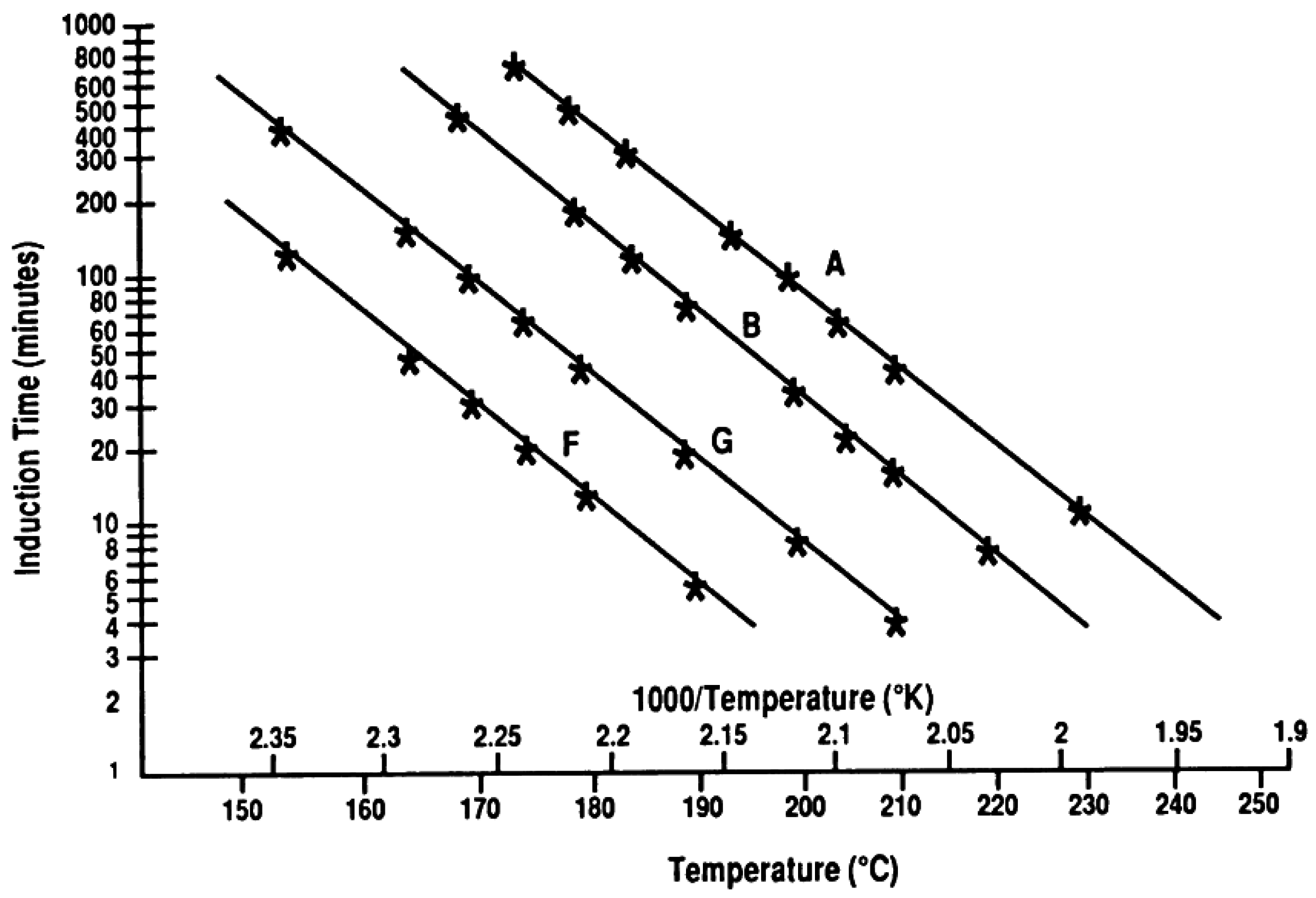
3.2.2. Kinetic Models

Kinetic models are used to estimate the induction times for grease in different temperatures. Induction time is used to compare the oxidation stability of different greases in any temperature, but cannot predict the oxidation life of grease. Almost all the kinetic models are first order, where the reaction rate coefficient is calculated from the Arrhenius law. In a first-order reaction, the reaction rate depends on the concentration of only one reactant. Mathematically, this is expressed as:

$$\frac{dC}{dt}= -kc.$$

(29)

Solving the above differential equation, we get

$$C=C_i{e}^{-kt},$$

(30)

where k is calculated from Arrhenius equation:

$$k=k_0{e}^{\frac{-E_a}{RT}},$$

(31)

where $E_a$ is the activation energy and $k_0$ is a constant. $E_a$ and $k_0$ are calculated experimentally, T is temperature, and R is the universal gas constant.

A zero-order reaction is a reaction whose rate does not depend on the concentration of reactants.

The rate equation has been solved for oxidation and evaporation of lubricating oil. Although the equation has not been solved for grease (because of the complexity of grease), examination of the oil models can provide good insight at least into the oxidation and evaporation of the base oil of grease.

Naidu et al. [29] presented a kinetic model for high-temperature oxidative degradation of a lubricant oil operating under the boundary lubrication conditions. They used a micro-oxidation test to study the oxidation of a thin layer of polyolester trimethylolpropane triheptanoate (TMPTH) oil as a simple reaction. A schematic of the apparatus is shown in Figure 6. It consists of a glass tube with a flat bottom and a gas inlet and outlet on the top. A small metal cup placed at the bottom of the test tube is filled with the sample oil, and the entire unit is immersed in a constant-temperature bath in the range between 150 °C and 245 °C. When the tube is purged with air both oxidation and evaporation occur, but the effect of evaporation is studied separately when only nitrogen gas is purged.

The products are then diluted with tetrahydrofuran and analyzed by gel permeation chromatography (GPC). The GPC analysis provides information on the molecular weight/size distribution of the products.

Figure 7 shows their oxidation model, where “A” represents the original oil, “E” the evaporated original oil (A) in the vapor phase, “B” the LMW (Low Molecular Weight) liquid-phase oxidation products, “F” the evaporated LMW products (B) in the vapor phase, “P” the HMW (High Molecular Weight) liquid-phase condensation polymerization products, and “D” sludge and varnish deposits. The constants $k_1$, $k_2$, and $k_5$ are first-order reaction rate constants. The constants $k_3$ and $k_4$ are composite evaporation rate constants. A diagram of the reaction scheme is shown in Figure 8.

They showed that the rate of evaporation can be assumed to be constant for their experiments. Therefore, according to [29]:

$$\mathrm{Rate} \mathrm{of} \mathrm{formation} \mathrm{of} \mathrm{B}=k_1{M}_A$$

$$\mathrm{Rate} \mathrm{of} \mathrm{reaction} \mathrm{of} \mathrm{B}=-k_2{M}_B$$

$$\mathrm{Rate} \mathrm{of} \mathrm{formation} \mathrm{of} \mathrm{P}=k_2{M}_B$$

$$\begin{gathered} \mathrm{rate} \mathrm{of} \mathrm{formation} \mathrm{of} \mathrm{D}=\mathrm{negligible} \mathrm{under} \mathrm{the} \mathrm{test} \mathrm{condition} \\ \left(\mathrm{as} \mathrm{the} \mathrm{sludge} \mathrm{formation} \mathrm{is} \mathrm{a} \mathrm{very} \mathrm{slow} \mathrm{process}\right) \end{gathered}$$

$$\mathrm{Rate} \mathrm{of} \mathrm{evaporation} \mathrm{of} \mathrm{A}=-k_3$$

$$\mathrm{Rate} \mathrm{of} \mathrm{evaporation} \mathrm{of} \mathrm{B}=-k_4,$$

where $M_A$ is the mass of the original oil A at any time t in the liquid form and $M_B$ is the mass of LMW product B. By defining $M_{A_0}$ as the mass fraction of the original oil present initially at the start of the test, and dividing all the mass fractions and evaporations rates by $M_{A_0}$ ($\overline{M}=\frac{M}{M_{A_0}},k^{*}=\frac{k}{M_{A_0}}$), these following equations are derived based on their oxidation model [29]:

$$\frac{d{\overline{M}}_A}{dt}=-k_3^{*}-k_1{\overline{M}}_A$$

(32)

$$\frac{d{\overline{M}}_B}{dt}=k_1{\overline{M}}_A-k_2{\overline{M}}_B-k_4^{*}$$

(33)

$$\frac{d{\overline{M}}_P}{dt}=k_2{\overline{M}}_B$$

(34)

$$\frac{d{\overline{M}}_E}{dt}=k_3^{*}$$

(35)

$$\frac{d{\overline{M}}_F}{dt}=k_4^{*}.$$

(36)

Naidu et al. solved the above equations with the initial conditions of:

$${\overline{M}}_B={\overline{M}}_P={\overline{M}}_E={\overline{M}}_F=0$$

(37)

$${\overline{M}}_A=1.$$

(38)

The solutions are:

$${\overline{M}}_A=\left[\frac{k_3^{*}}{k_1}+1\right]e^{-k_{1}t}-\frac{k_3^{*}}{k_1}$$

(39)

$${\overline{M}}_B=\left[\frac{k_3^{*}+k_4^{*}}{k_2}\right][e^{-k_{2}t}-1]+\left[\frac{k_3^{*}+k_1}{k_2-k_1}\right][e^{-k_{1}t}-e^{-k_{2}t}]$$

(40)

$${\overline{M}}_P=[k_3^{*}+k_4^{*}][\frac{1-e^{-k_{2}t}}{k_2}-t]+\left[\frac{k_2\left(k_3^{*}+k_1\right)}{k_2-k_1}\right][\frac{1-e^{-k_{1}t}}{k_1}-\frac{1-e^{-k_{2}t}}{k_2}]$$

(41)

$${\overline{M}}_E=k_3^{*}t$$

(42)

$${\overline{M}}_F=k_4^{*}t.$$

(43)

The mass fraction of original oil remaining ($M_A$) and the mass fraction of HMW products (${\overline{M}}_P$) are determined from GPC analysis of the oxidation products. ${\overline{M}}_E$ and $k_3^{*}$ are measured from the evaporation test. ${\overline{M}}_F$ is calculated from the mass balance equation. It was shown that in all cases $k_2$ was at least 100 times larger than $k_1$, which means the rate of polymerization (HMW production from LMW products) is much higher than the rate of LMW products formation. Therefore, ${\overline{M}}_B$ approximately is equal to zero, and Equation (41) can be simplified as:

$${\overline{M}}_P=[k_3^{*}+k_4^{*}]\left(-t\right)+\left[\frac{\left(k_3^{*}+k_1\right)}{k_1}\right]\left(1-\exp \left(k_{1}t\right)\right).$$

(44)

Oxidation and evaporation tests were conducted at 150, 185, 200, 225, and 245 °C. Arrhenius plots for $k_1$, $k_3^{*}$, and $k_4^{*}$ are shown in Figure 9.

$k_1$ is constant for all the temperatures; $k_3^{*}$ and $k_4^{*}$ change slightly with the temperature.

A comparison between the model prediction and the experimental data is shown in Figure 10 for 185 °C [29].

It appears that, for the most part, the data predicted by the model agree reasonably well with the experimental data. The following conclusions can be drawn from Naidu et al. [29]:

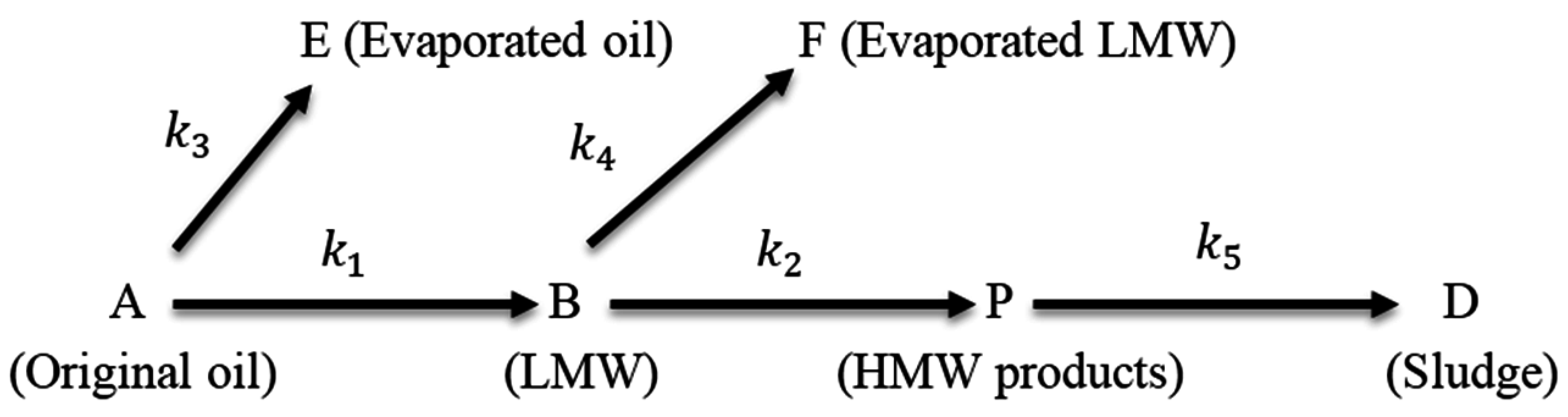
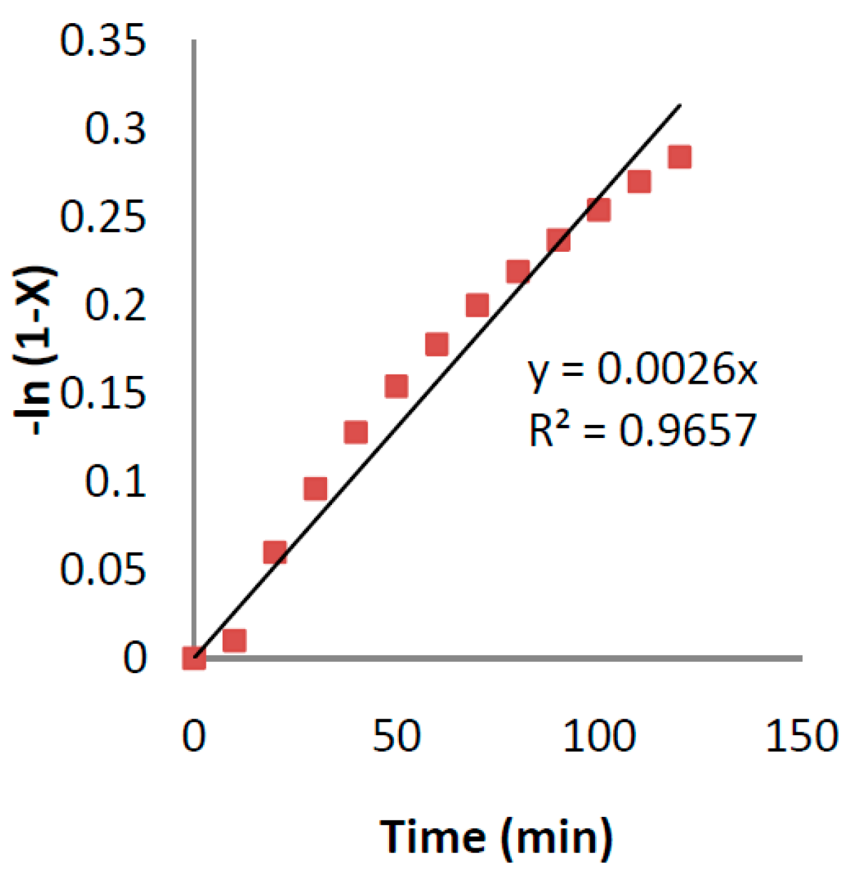
• The first-order kinetic model seems to fit well with the oxidation of the lubricant;
• The zero-order kinetic model seems to fit well with the evaporation of the base oil and LMW products;
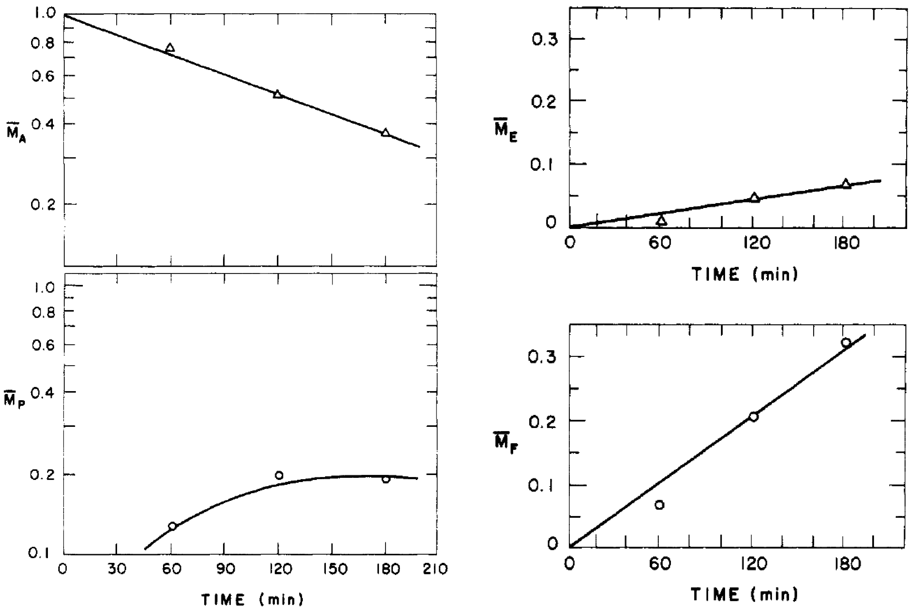
• The mass fraction of the original oil (MA) decreases almost linearly with time from the first moment of the process;
• The mass fraction of evaporated oil (ME) and evaporated LMW products (MF) increase linearly with time from the first moment of the process;
• The mass fraction of HMW products (MP) increases exponentially with time. There is not any HMW product formation for a while at the beginning of the process. It can be concluded that the oxidation inhibitors’ scarification prevents the polymerization of the radicals in this induction phase; and
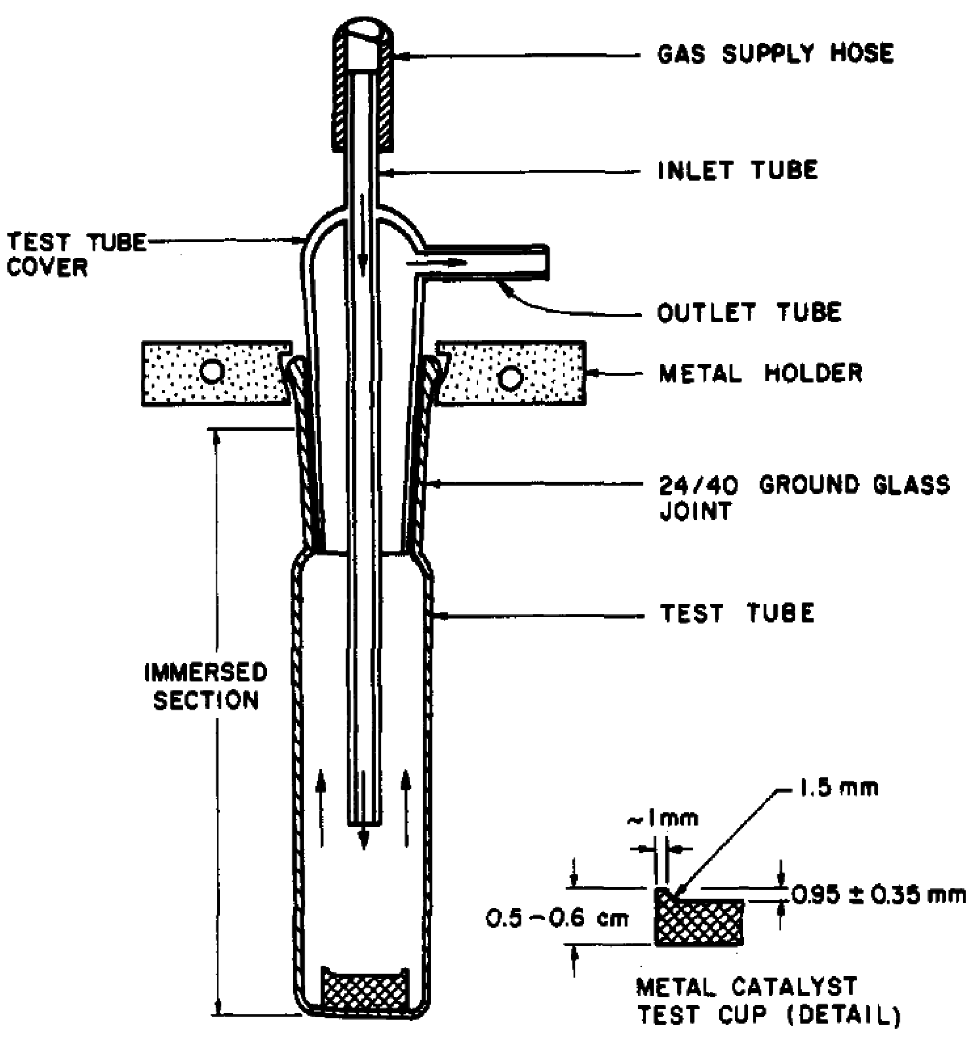
• Because of the small size of oil sample, the model neglects the effect of oxygen diffusion. However, the oxidation rate can be limited by the oxygen diffusion mechanism in real applications. Therefore, the model underestimates the life of the lubricant in larger size samples.

Gimzewski [30] also used a first-order kinetic model (by considering a constant mass fraction for oxygen) to derive an equation that relates induction times and induction temperatures in two different DSC tests (isothermal mode to measure induction times at a constant temperature and scanning mode to measure induction temperatures when temperature is rising with a rate of $\beta =\frac{dT}{dt}$).

He considered fully formulated products that include primary oxidation inhibitors—such as hindered phenols or aromatic amines, which remove peroxyl radicals (ROO*)—and secondary oxidation inhibitors—such as zinc dialkyl dithiophosphate, which decompose the autocatalytic hydroperoxides (ROOH)—and assumed that the oxidation rate of a thin film of oil in a DSC experiment is limited by the chain initiation reaction (Equation (45)) rate when either type of inhibitor reaches a critically low value.

$$RH+O_2\to R^{*}+H{O_2}^{*}$$

(45)

The corresponding rate equation for Equation (45) is:

$$-\frac{d\left[RH\right]}{dt}=\left[RH\right]\left[O_2\right]Aexp\left(-\frac{E_a}{RT}\right).$$

(46)

Gimzewski [30] wrote the rate equation for both types of DSC test modes, and by separating the variables and assuming an equal [RH] induction in both cases, he derived the following relation to estimate an oxidation induction time for an isothermal run at T_iso to the oxidation induction temperature for a scanning run at a heating rate of β:

$$t_{ind}=[1/[\exp \left(-\frac{E_a}{R{T}_{iso}}\right)\beta ]]{{\displaystyle \int }}_0^{T_{ind}}\exp \left(-\frac{E_a}{RT}\right)dT.$$

(47)

He assumed an activation energy $E_a$ of 140 kJ/mol and performed tests on 16 lubricating oils, two gasolines, and one grease. His analytical results showed agreement with experimental results, with less than 15% error. He also measured the activation energy by performing DSC tests in different temperatures and using the Arrhenius equation for four different oils. All the activation energies fell in the range of 140 ± 30 kJ/mol. Equation (47) is used to select the optimum test temperature for a DSC isothermal oxidation test by performing a scanning DSC test. The lubricant will oxidize in a reasonable induction time when the test is performed at the optimum test temperature. Gimzewski’s work is not a life estimation model, but showed that considering an activation energy of 140 kJ/mol is a good assumption for most lubricants.

Rhee [33] also used a first-order kinetic model for grease oxidation. He used PDSC to measure the induction time in different temperatures for four different greases and showed an Arrhenius plot of the results (plotting induction times in a natural logarithmic vertical axis versus reciprocal related test temperatures in the horizontal axis). He showed that the results are linear with almost the same slope for all the greases (Figure 11).

He concluded that a first-order kinetic model fits the grease oxidation well —because of the linearity—and the activation energy (the slope of the lines in the Arrhenius plot) is independent of the grease type and is almost 146 kJ/mol. From Figure 11 the induction time can be expressed as:

$$\ln \left(t\right)=\ln \left(A\right)+E/RT,$$

(48)

where $T$ is temperature, $E$ is the activation energy, $R$ is gas constant, 8.314 J/mol K, and $A$ is the oxidation coefficient of grease, which is constant and different for every grease. Assuming a value of 146 kJ/mol for activation energy, Equation (48) can be simplified to:

$$t=\mathrm{A}\exp \left(17500/T\right).$$

(49)

The oxidation coefficient for grease may be calculated by solving Equation (49) for A, using a known induction time.

3.2.3. Chemical Life Estimating Models

Despite the existence of rich volumes of published works on the chemical degradation monitoring and kinetic models, a practical chemical life estimating model is still unavailable.

Rhee attempted to utilize his kinetic model to develop a grease life prediction model. In his later work [34], he addressed two limitations of his kinetic model: limited ability to predict the induction time due to inaccurate activation energy determination, and the need to estimate the oxidation life of grease in a PDSC test.

To address the first limitation, he suggested measuring two induction times (t₁ and t₂) at two different temperatures (T₁ and T₂) and finding the activation energy for any grease from Equation (49):

$$E=R\frac{T_1{T}_2}{T_1-T_2}\ln \left(\frac{t_1}{t_2}\right).$$

(50)

To address the second limitation, he developed an empirical relation between the experimentally measured, high-temperature grease life and induction time by curve fitting. The experimental grease life were obtained from testing the grease in an automotive wheel bearing test rig at 160 °C based on ASTM D 3527 standard test method [41]. The empirical relation is:

$$\mathrm{Grease}\mathrm{High}\mathrm{Temperature}\mathrm{Life}\left(\mathrm{h}\right)=177t^{0.31}.$$

(51)

Equation (51) was tested for 10 grease samples. The results are shown in

Table 1. Comparison between actual grease life and predicted grease life using Equation (51) [34].

Sample	ASTM D 3527, h	Predicted Grease Life, h	Oil Separation @ 180 °C, %
A	151	150	25.9
B	340	368	2.9
C	400	395	4.4
D	240	228	13.2
E	171	191	12.0
F	100	313	82.3
G	192	186	12.7
H	20	200	31.8
I	40	158	52.9
J	287	266	3.6

.

Three grease samples’ life (F, H, and I) show a significant difference with the life predicted by Equation (51). It was concluded that these greases have a thermal stability problem at the tested temperature, which causes excessive oil separation and evaporation; also, because ASTM D3527 test is a dynamic test, the excessive oil does not remain in the bearing, whereas in PDSC (which is a static test) the separated oil is still present. Therefore, Rhee suggested using the model for the greases with less than 30% oil separation at 180 °C. However, the predicted life for grease A with 25.9% oil separation still shows good agreement with ASTM D3527 experimental results. Note that this model neglects the physical degradation (such as evaporation and mechanical grease degradation) of grease in a dynamic application such as ASTM D 3527 test. This may explain the discrepancy since a grease with good chemical stability may still suffer from physical degradation.

Rhee addressed the oil separation and evaporation in his later work [35] by adding a decomposition model to his kinetic model. He measured the grease weight decrease from base oil evaporation and separation using a modified Thermogravimetric Analyzer (TGA). TGA is normally used to measure the evaporative weight decrease of materials in high temperatures. By punching pinholes in the TGA pan to collect the separated oil, he successfully measured the total evaporative and oil separation weight losses. Rhee considered a first-order kinetic model for grease evaporation and oil separation and, similar to his derivation of the kinetic model, he derived an equation based on the Arrhenius law. Then, he combined the decomposition model, which was based on TGA, with the kinetic model, which was based on PDSC, and came up with the following decomposition kinetic model:

$$t\left(\mathrm{h}\right)={\left[\frac{\frac{4.6}{k_0}{e}^{\frac{E}{RT}}}{60}\right]}^{\alpha },$$

(52)

where $\alpha =\frac{t_i}{120}$ and t_i: Induction time in PDSC at test temperature. If t_i > 120, then α = 1.

The parameters $k_0$ and $E$ are calculated based on TGA results in two different temperatures. Rhee subsequently derived the following empirical relation by comparing the new decomposition kinetic model by ASTM D 3527 results:

$$\mathrm{Grease}\mathrm{High}\mathrm{Temperature}\mathrm{Life}\left(\mathrm{h}\right)=65t^{0.32}$$

(53)

Equation (53) was also tested for 10 grease samples. The results are shown in

Table 2. Comparison between actual grease life (ASTM D 3527) and predicted grease life using Equation (53) [35].

Sample	Kinetic Life @180 °C, h	ASTM D3527, h	Predicted Grease Life, h
A	19.1	150	167
B	59	240	240
C	21.2	170	174
D	0.02	20	18.6
E	20.7	196	171
F	4.6	100	106
G	30	192	194
H	7.29	120	123
I	0.25	40	41
J	108	275	290

.

With this new relation, the results are more promising for F, H, and I greases. However, for grease A the model overestimated grease life. This new model is empirically derived and still ignores the mechanical grease degradation. The linear curve fit to the TGA results based on the assumption of a first-order kinetic model is shown in Figure 12.

Since the trend of the curve is not completely linear, the assumption of a first-order kinetic model for base oil separation and evaporation may not be very accurate. Naidu et al. [29] used a zero-order kinetic model for the base oil evaporation. Oil separation/bleeding has been related to the base oil/thickener combination and kinematic viscosity of the base oil [42] or to the viscous flow of the base oil through the porous microstructure of the thickener [43].

4. Summary and Conclusions

Table 3. Summary of the literature on grease degradation and life prediction.

Empirical models	[6,7,8,9,10,41,44,45]
Physical Degradation	Mechanical degradation	Monitoring	SEM [13,25,46,47,48]
			Penetration [12,49,50]
			Shear stress [13,14]
		Shear stress functions	Empirical [14,15,16]
			Analytical [13,22]
		Mechanical stability [14,17,19,20,46,51,52,53]
		Life predicting models [13]
	Base oil evaporation [42,48,50]
	Base oil separation/Grease leakage [25,42,43]
	Contamination [54]
Chemical Degradation	Monitoring	DSC/PDSC [23,30,33,34,35,36,55]
		FTIR [11,25,47,48,54,55,56,57,58,59,60]
		Acid number [25,50,55]
		Ruler [55,61,62]
		Thermogravimetry [42,63]
		gel permeation chromatography [25,29,48]
	Kinetic models [23,29,30,33,35,63]
	Chemical stability [33,36]
	Life predicting models [34,35,63]
Grease Flow	Film thickness measurement [47,54,58,59,64,65,66]
	Starvation [54,64,65,66]

provides a summary of grease life degradation and life prediction. In some categories, because of the similarity, only some of the studies referenced in Table 3 were described in this paper. Although this paper is a summary of the literature on grease degradation and life prediction, some papers on grease flow that may include useful related information to the topic of this paper are also listed in Table 3.

The following conclusions are drawn from the literature review:

• Mechanical and chemical degradation are important grease degradation mechanisms.
• Mechanical and chemical degradation are irreversible processes.
• Mechanical degradation can be addressed from an energy/entropy point of view.
• Chemical degradation has been studied applying a first-order kinetic model.
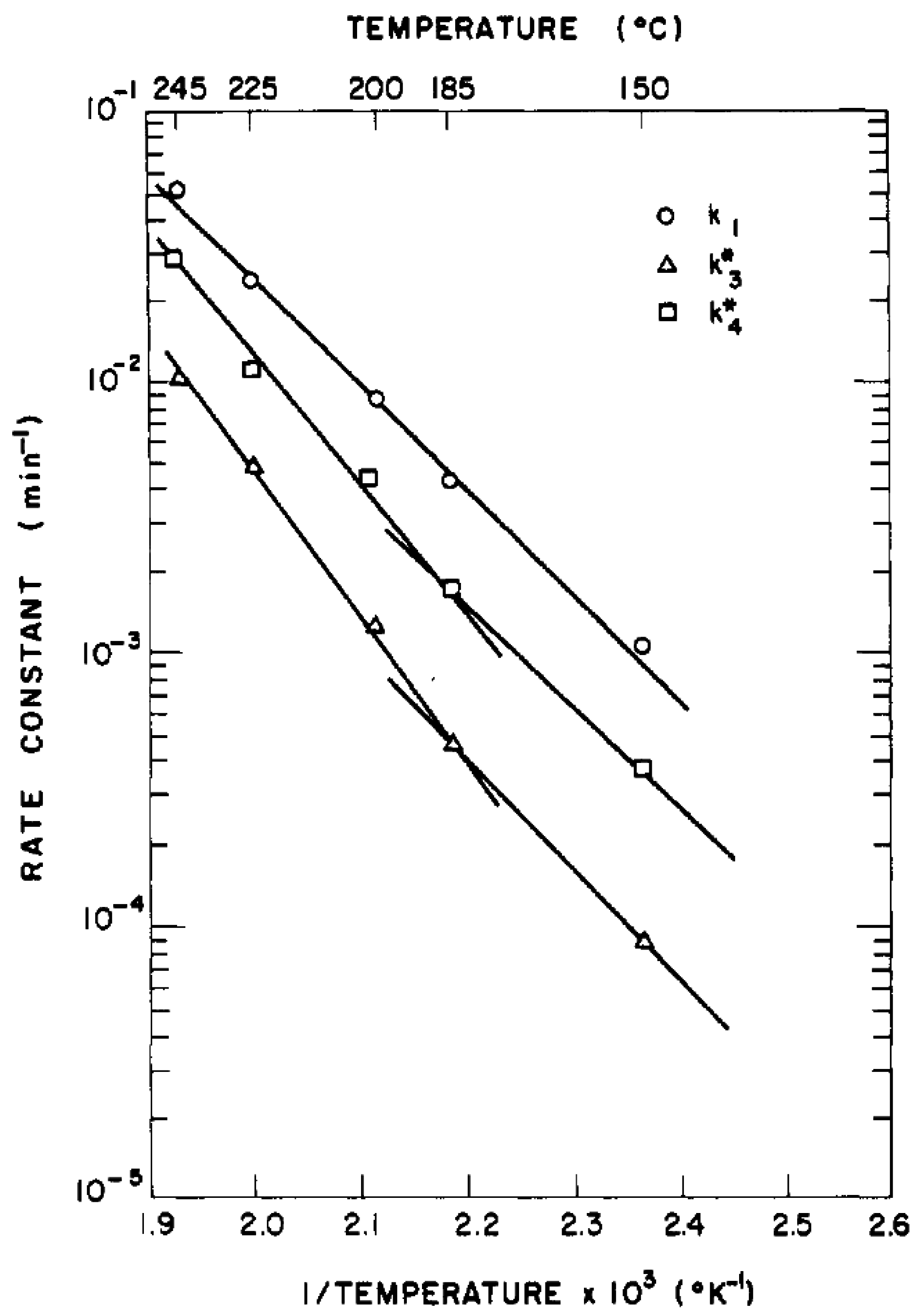
• Arrhenius’ law has been used to calculate the activation energy and reaction rate in the applied first-order kinetic model.
• Chemical degradation is controlled by the activation energy provided to grease, and can be studied from an energy/entropy point of view.
• Mechanical and chemical degradation occur simultaneously in real applications.

References

1. Barnett, R. Review of recent USA publications on lubricating grease. Wear 1970, 16, 87–142. [Google Scholar] [CrossRef]
2. Langborne, P. Grease lubrication: A review of recent british papers. In Proceedings of the Institution of Mechanical Engineers, Conference Proceedings September 1969; SAGE Publications: Thousand Oaks, CA, USA, 1969; pp. 82–86. [Google Scholar]
3. Rush, R.E. A review of the more common standard grease tests in use today. Tribol. Lubr. Technol. 1997, 53, 17. [Google Scholar]
4. Lugt, P.M. A review on grease lubrication in rolling bearings. Tribol. Trans. 2009, 52, 470–480. [Google Scholar] [CrossRef]
5. Lugt, P.M. Grease Lubrication in Rolling Bearings; John Wiley & Sons: Hoboken, NJ, USA, 2012. [Google Scholar]
6. Booser, E. Grease life forecast for ball-bearings. Lubr. Eng. 1974, 30, 536–541. [Google Scholar]
7. Kawamura, T.; Minami, M.; Hirata, M. Grease life prediction for sealed ball bearings. Tribol. Trans. 2001, 44, 256–262. [Google Scholar] [CrossRef]
8. Booser, R.; Khonsari, M. Grease life in ball bearings: The effect of temperatures. Tribol. Lubr. Technol. 2010, 66, 36–44. [Google Scholar]
9. Booser, E.; Khonsari, M. Systematically selecting the best grease for equipment reliability. Mach. Lubr. 2007, 1, 19–25. [Google Scholar]
10. Booser, E.; Khonsari, M. Grease and grease life. In Encyclopedia of Tribology; Springer: Berlin, Germany; Heidelberg, Germany, 2013; pp. 1555–1561. [Google Scholar]
11. Cann, P.M.; Doner, J.P.; Webster, M.N.; Wikstrom, V. Grease degradation in rolling element bearings. Tribol. Trans. 2001, 44, 399–404. [Google Scholar] [CrossRef]
12. Rezasoltani, A.; Khonsari, M. On the correlation between mechanical degradation of lubricating grease and entropy. Tribol. Lett. 2014, 56, 197–204. [Google Scholar] [CrossRef]
13. Rezasoltani, A.; Khonsari, M. An engineering model to estimate consistency reduction of lubricating grease subjected to mechanical degradation under shear. Tribol. Int. 2016, 103, 465–474. [Google Scholar] [CrossRef]
14. Kuhn, E. Experimental grease investigations from an energy point of view. Ind. Lubr. Tribol. 1999, 51, 246–251. [Google Scholar] [CrossRef]
15. Bauer, W.H.; Finkelstein, A.P.; Wiberley, S.E. Flow properties of lithium stearate-oil model greases as functions of soap concentration and temperature. ASLE Trans. 1960, 3, 215–224. [Google Scholar] [CrossRef]
16. Czarny, R. Effects of changes in grease structure on sliding friction. Ind. Lubr. Tribol. 1995, 47, 3–7. [Google Scholar] [CrossRef]
17. Kuhn, E. Description of the energy level of tribologically stressed greases. Wear 1995, 188, 138–141. [Google Scholar] [CrossRef]
18. Kuhn, E.; Balan, C. Experimental procedure for the evaluation of the friction energy of lubricating greases. Wear 1997, 209, 237–240. [Google Scholar] [CrossRef]
19. Kuhn, E. Investigations into the degradation of the structure of lubricating greases. Tribol. Trans. 1998, 41, 247–250. [Google Scholar] [CrossRef]
20. Kuhn, E. Analysis of a grease-lubricated contact from an energy point of view. Int. J. Mater. Prod. Technol. 2010, 38, 5–15. [Google Scholar] [CrossRef]
21. Kuhn, E. Friction and wear of a grease lubricated contact—An energetic approach. In Tribology-Fundamentals and Advancements; Gegner, J., Ed.; InTech: Rijeka, Croatia, 2013. [Google Scholar]
22. Spiegel, K.; Fricke, J.; Meis, K.-R. Die Flieûeigenschaften von Schmierfetten in Abhaè Ngigkeit von Beanspruchung, Beanspruchungsdauer und Temperatur; Bartz, W.J., Ed.; Tribology 2000: Esslingen, Germany, 1989. [Google Scholar]
23. Rohrbach, P.; Hamblin, P.; Ribeaud, M. Benefits of antioxidants in lubricants and greases assessed by pressurised differential scanning calorimetry. Tribotest 2005, 11, 233–246. [Google Scholar] [CrossRef]
24. Booser, E.R. Tribology Data Handbook: An Excellent Friction, Lubrication, and Wear Resource; CRC Press: Boca Raton, FL, USA, 2010. [Google Scholar]
25. Ito, H.; Tomaru, M.; Suzuki, T. Physical and chemical aspects of grease deterioration in sealed ball bearings. Lubr. Eng. 1988, 44, 872–879. [Google Scholar]
26. Reyes-Gavilan, J. Evaluation of the thermo-Oxidative Characteristics of Greases by Pressurized Differential Scanning Calorimetry; NLGI Spokesman-Including NLGI Annual Meeting-National Lubricating Grease Institute; National Lubricating Grease Institute: Kansas City, MO, USA, 2004; pp. 20–27. [Google Scholar]
27. Cousseau, T.; Graça, B.; Campos, A.; Seabra, J. Grease aging effects on film formation under fully-flooded and starved lubrication. Lubricants 2015, 3, 197–221. [Google Scholar] [CrossRef]
28. Gonçalves, D.; Graça, B.; Campos, A.V.; Seabra, J. Film thickness and friction behaviour of thermally aged lubricating greases. Tribol. Int. 2016, 100, 231–241. [Google Scholar] [CrossRef]
29. Naidu, S.; Klaus, E.; Duda, J. Kinetic model for high-temperature oxidation of lubricants. Ind. Eng. Chem. Prod. Res. Dev. 1986, 25, 596–603. [Google Scholar] [CrossRef]
30. Gimzewski, E. The relationship between oxidation induction temperatures and times for petroleum products. Thermochim. Acta 1992, 198, 133–140. [Google Scholar] [CrossRef]
31. Sharma, B.K.; Stipanovic, A.J. Development of a new oxidation stability test method for lubricating oils using high-pressure differential scanning calorimetry. Thermochim. Acta 2003, 402, 1–18. [Google Scholar] [CrossRef]
32. Bowman, W.; Stachowiak, G. Determining the oxidation stability of lubricating oils using sealed capsule differential scanning calorimetry (scdsc). Tribol. Int. 1996, 29, 27–34. [Google Scholar] [CrossRef]
33. Rhee, I.-S. Development of a new oxidation stability test method for greases using a pressure differential scanning calorimeter. In Proceedings of the NLGI’s 57th Annual Meeting, Denver, CO, USA, 2–6 July 1990.
34. Rhee, I.-S. Decomposition Kinetic of Greases by Thermal Analysis; DTIC Document; Tacom Research Development and Engineering Center: Warren, MI, USA, 2007. [Google Scholar]
35. Rhee, I.-S. Prediction of High Temperature Grease Life Using a Decomposition Kinetic Model; DTIC Document; Army Tank-Automotive Research and Development Center: Warren, MI, USA, 2009. [Google Scholar]
36. ASTM. D5483, Standard Test Method for Oxidation Induction Time of Lubricating Greases by Pressure Differential Scanning Calorimetry; ASTM International: West Conshohocken, PA, USA, 1993. [Google Scholar]
37. Van De Voort, F.; Sedman, J.; Cocciardi, R.; Pinchuk, D. Ftir condition monitoring of in-service lubricants: Ongoing developments and future perspectives. Tribol. Trans. 2006, 49, 410–418. [Google Scholar] [CrossRef]
38. ASTM. D974, Standard Test Method for Acid and Base Number by Color-Indicator Titration; ASTM International: West Conshohocken, PA, USA, 2002. [Google Scholar]
39. ASTM. D664, Standard Test Method for Acid Number of Petroleum Products by Potentiometric Titration; ASTM International: West Conshohocken, PA, USA, 2011. [Google Scholar]
40. Freepik, E.R. TutsPlus. Ruler Testing. Available online: http://mrgcorp.com/ (accessed on 230June 2016).
41. ASTM. Standard test method for life performance of automotive wheel bearing grease. In D3527; ASTM International: West Conshohocken, PA, USA, 2015. [Google Scholar]
42. Yokoyama, F. Optimization of grease properties to prolong the life of lubricating greases. J. Phys. Sci. Appl. 2014, 4, 236–247. [Google Scholar]
43. Baart, P.; van der Vorst, B.; Lugt, P.M.; van Ostayen, R.A. Oil-bleeding model for lubricating grease based on viscous flow through a porous microstructure. Tribol. Trans. 2010, 53, 340–348. [Google Scholar] [CrossRef]
44. Ito, H.; Koizumi, H.; Naka, M. Grease life equations for sealed ball bearings. In Proceedings of the International Tribology Conference, Yokohama, Japan, 29 October–2 November 1995; pp. 931–936.
45. Tomaru, M.; Suzuki, T.; Ito, H.; Suzuki, T. Grease-life estimation and grease deterioration in sealed ball bearings. In Proceedings of the JSLE International Tribology Conference, Tokyo, Japan, 8–10 July 1985; pp. 1039–1044.
46. Paszkowski, M. Some aspects of grease flow in lubrication systems and friction nodes. In Tribology—Fundamentals and Advancements; InTech: Rijeka, Croatia, 2013; pp. 77–106. [Google Scholar]
47. Huang, L.; Guo, D.; Cann, P.; Wan, G.T.Y.; Wen, S. Thermal oxidation mechanism of polyalphaolefin greases with lithium soap and diurea thickeners: The effects of the thickener. Tribol. Trans. 2016, 59, 801–809. [Google Scholar] [CrossRef]
48. Araki, C.; Kanzaki, H.; Taguchi, T. A study on the thermal degradation of lubricating greases. NLGI Spokesm. 1995, 59, 15–23. [Google Scholar]
49. ASTM. Standard test methods for cone penetration of lubricating grease. In D217-10; ASTM International: West Conshohocken, PA, USA, 2010. [Google Scholar]
50. Komatsuzakl, S.; Uematsu, T.; Kobayashl, Y. Change of grease characteristics to the end of lubricating life. NLGI Spokesm. 2000, 63, 22–29. [Google Scholar]
51. Lundberg, J.; Höglund, E. A new method for determining the mechanical stability of lubricating greases. Tribol. Int. 2000, 33, 217–223. [Google Scholar] [CrossRef]
52. Kuhn, E. Correlation between system entropy and structural changes in lubricating grease. Lubricants 2015, 3, 332–345. [Google Scholar] [CrossRef]
53. Lundberg, J.; Parida, A.; Söderholm, P. Running temperature and mechanical stability of grease as maintenance parameters of railway bearings. Int. J. Autom. Comput. 2010, 7, 160–166. [Google Scholar] [CrossRef]
54. Hurley, S.; Cann, P.; Spikes, H. Lubrication and reflow properties of thermally aged greases. Tribol. Trans. 2000, 43, 221–228. [Google Scholar] [CrossRef]
55. Aranzabe, A.; Aranzabe, E.; Marcaide, A.; Ferret, R.; Terradillos, J.; Ameye, J.; Shah, R. Comparing Different Analytical Techniques to Monitor Lubricating Grease Degradation; NLGI Spokesman-Including NLGI Annual Meeting-National Lubricating Grease Institute; National Lubricating Grease Institute: Kansas City, MO, USA, 2006; pp. 17–30. [Google Scholar]
56. Cann, P.; Webster, M.; Doner, J.; Wikstrom, V.; Lugt, P. Grease degradation in r0f bearing tests. Tribol. Trans. 2007, 50, 187–197. [Google Scholar] [CrossRef]
57. Cann, P. Grease lubrication of rolling element bearings—Role of the grease thickener. Lubr. Sci. 2007, 19, 183–196. [Google Scholar] [CrossRef]
58. Hurley, S.; Cann, P.; Spikes, H. Thermal degradation of greases and the effect on lubrication performance. Tribol. Ser. 1998, 34, 75–83. [Google Scholar]
59. Cann, P. Grease degradation in a bearing simulation device. Tribol. Int. 2006, 39, 1698–1706. [Google Scholar] [CrossRef]
60. Carré, D.; Bauer, R.; Fleischauer, P. Chemical analysis of hydrocarbon grease from spin bearing tests. ASLE Trans. 1983, 26, 475–480. [Google Scholar] [CrossRef]
61. Maguire, E. Monitoring of Lubricant Degradation with RULER and MPC. Master’s Thesis, Linköping University, Linköping, Sweden, 2010. [Google Scholar]
62. Fentress, A.; Ameye, J.; Sander, J. The use of linear sweep voltammetry in condition monitoring of diesel engine oil. J. ASTM Int. 2011, 8, 1–10. [Google Scholar] [CrossRef]
63. Ide, A.; Asai, Y.; Takayama, A.; Akiyama, M. New life prediction method of the grease by the activation energy. Tribol. Online 2011, 6, 45–49. [Google Scholar] [CrossRef]
64. Vengudusamy, B.; Kuhn, M.; Rankl, M.; Spallek, R. Film forming behavior of greases under starved and fully flooded ehl conditions. Tribol. Trans. 2016, 59, 62–71. [Google Scholar] [CrossRef]
65. Hoglund, E. Lubricating grease replenishment in an elastohydrodynamic point contact. J. Tribol. 1993, 115, 501. [Google Scholar]
66. Cann, P. Starvation and reflow in a grease-lubricated elastohydrodynamic contact. Tribol. Trans. 1996, 39, 698–704. [Google Scholar] [CrossRef]
Figure 1. Guidelines for bearing re-greasing intervals with mild operating conditions [10].
Lubricants 04 00034 g001
Figure 2. SEM image of XHP222 soap network after washing out the base oil.
Lubricants 04 00034 g002
Figure 3. SEM image of XHP222 soap network after 15 h shearing with a shear rate of 5000 1/s.
Lubricants 04 00034 g003
Figure 4. Shear stress decrease vs. time for XHP222 grease during a constant shear rate of 2500 1/s and at a constant temperature of 35 °C [13].
Lubricants 04 00034 g004
Figure 5. Spiegel et al. model [22].
Lubricants 04 00034 g005
Figure 6. Micro-oxidation test apparatus [29].
Lubricants 04 00034 g006
Figure 7. Naidu et al. oxidation model [29].
Lubricants 04 00034 g007
Figure 8. Diagram of the reaction scheme [29].
Lubricants 04 00034 g008
Figure 9. Arrhenius plots for k 1 , k 3 * , and k 4 * [29].
Lubricants 04 00034 g009
Figure 10. Comparison between the model prediction and the experimental data for 185 °C [29].
Lubricants 04 00034 g010
Figure 11. Arrhenius plots for four different greases [33].
Lubricants 04 00034 g011
Figure 12. Linear curve fit to the TGA results based on the assumption of a first-order kinetic model [35].
Lubricants 04 00034 g012