Tracing Primordial Magnetic Fields with 21 cm Line Observations

Abstract

Magnetic fields are observed on a large range of scales in the universe. Up until recently, the evidence always pointed to magnetic fields associated with some kind of structure, from planets to clusters of galaxies. Blazar observations have been used to posit the first evidence of truly cosmological magnetic fields or void magnetic fields. A cosmological magnetic field generated in the very early universe before recombination has implications for the cosmic microwave background (CMB), large scale structure as well as the 21 cm line signal. In particular, the Lorentz term causes a change in the linear matter power spectrum. Its implication on the 21 cm line signal was the focus of our recent simulations which will be summarised here. Modelling the cosmological magnetic field as a gaussian random field numerical solutions were found for magnetic fields with present day amplitudes of 5 nG and negative spectral indices which are within the range of observational constraints imposed by the cosmic microwave background (CMB).

1. Introduction

There are undisputed observations of magnetic fields associated with upto the largest structures such as clusters of galaxies (cf., e.g., [1,2,3,4,5,6,7]). In addition, still under debate are void magnetic fields from observations of a number of blazar energy spectra in the TeV and the GeV ranges. These observations actually provide, in the simplest models, lower limits on the magnetic field strength and in more complicated ones impose a range of magnetic field values. Depending on the models values are of the order of ${10}^{-25}$–10${}^{-15}$ nG (e.g., [8,9,10,11]) which are significantly below magnetic field strengths found in galaxies which are of the order of ${10}^{-6}$ G (e.g., [12]). Void magnetic fields, not associated with any virialized structure, are very interesting since they could be evidence for the existence of truly cosmological magnetic fields. Such fields could serve as seeds for galactic magnetic fields if generated in the early universe. There is a large class of mechanisms which generate magnetic fields in the very early universe long before recombination. This is divided into two subclasses, one comprises inflationary models and the other from phase transitions (for reviews, cf., e.g., [13,14]).

The cosmic microwave background (CMB) has a nearly perfect black body spectrum at a present temperature $T_0=2.73$ K with only tiny fluctuations superimposed which are of the order of $\Delta T/T_0\sim {10}^{-5}$. This global isotropy rules out a strong homogeneous magnetic field on large scales as it signals out a preferred direction. Limits of a few nG have been obtained from current observations, taking into account this breaking of isotropy by assuming a Bianchi I model for the background [15,16]. Models of magnetogenesis typically predict random magnetic fields [17]. This motivates us to treat a putative cosmological magnetic field as a stochastic, random, Gaussian field. The anisotropies imprinted on the CMB are determined by the interaction and evolution of the perturbations in the physical quantities in the different matter components of the cosmic plasma, such as baryons, neutrinos and photons. Including a stochastic magnetic field in the very early universe, before recombination, implies additional contributions to the total energy density perturbations, anisotropic stress and the evolution equation of the baryon velocity. In the latter the Lorentz term which couples to the ionized matter part has to be included. This leads to additional power in the linear matter density power spectrum on small scales, e.g., cf., [18].

Generating magnetic fields during inflation relies on similar mechanisms as the one for generating the primordial curvature mode required to explain the observed CMB anisotropy in temperature and polarization angular power spectra. Thus stochastic magnetic fields are generated by amplification of perturbations in the electromagnetic filed on superhorizon scales. However, within these models additional assumptions have to be made in order to break conformal invariance of linear electrodynamics. Otherwise the magnetic field amplitudes are too small to be cosmologically relevant. There is no problem generating magnetic fields with large enough correlation length which is a critical point for mechanisms operating during phase transitions. In this latter class of models, the resulting magnetic fields can have strong amplitudes. Moreover, recent simulations of the evolution of magnetic fields generated during the electroweak phase transition indicate that decaying helical MHD turbulence leads to a significant increase in correlation length via inverse cascade [19]. Finally it should also be mentioned that magnetic fields resulting from phase transitions generically are helical magnetic fields, and those from inflationary mechanisms are non helical (for a review, cf. e.g., [13,14]).

The 21 cm line signal is caused by the hyperfine transition of the ground state of neutral hydrogen atoms. Its brightness temperature is observed against a background radiation field which in the cosmological context usually is assumed to be the CMB. When CMB photons travel through a region of neutral hydrogen some of them will be absorbed by atoms in the lower energetic singlet state exciting them to the higher energetic triplet state. Other hydrogen atoms will be in the triplet state and relaxing down to the singlet state by spontaneous emission. Taking into account that the environment is optically thin and redshifts $z\gg 1$ the change in the brightness temperature of the CMB, $\delta T_b=T_b-T_{CMB}$, is given by [20,21]

$$\begin{array}{c}\hfill \delta T_b=28\mathrm{mK}\left(\frac{{\mathsf{\Omega }}_{b,0}h}{0.03}\right){\left(\frac{{\mathsf{\Omega }}_{m,0}}{0.3}\right)}^{-\frac{1}{2}}{\left(\frac{1+z}{10}\right)}^{\frac{1}{2}}\frac{\left(T_S-T_{CMB}\right)}{T_S}{x}_{HI},\end{array}$$

(1)

where ${\mathsf{\Omega }}_{b,0}$ and ${\mathsf{\Omega }}_{m,0}$ are the present day baryon and matter density parameters, respectively. The value $x_{HI}$ denotes the fraction of neutral hydrogen. The spin temperature $T_S$ is defined as the equilibrium temperature of the ratio of the number densities in the triplet and singlet states of the ground state of hydrogen, $n_1$ and $n_0$, respectively, by

$$\begin{array}{c}\hfill \frac{n_1}{n_0}=3exp\left(-\frac{T_{*}}{T_S}\right)\end{array}$$

(2)

where $T_{*}=68$ mK corresponds to the energy difference between the two hyper fine levels of the ground state. The 21 cm signal is observed in absorption or emission depending on whether the spin temperature is higher or lower than the temperature of the CMB. When CMB photons pass through a region of neutral hydrogen they might be absorbed and/or cause stimulated emission which changes the ratio of number densities in the singlet and triplet states, respectively, and thus the spin temperature. However, on a time scale much shorter than the age of the universe after recombination the spin temperature equalises with the temperature of the CMB. There are two additional processes which could break this coupling between $T_S$ and $T_{CMB}$. Firstly, earlier on, at higher redshifts gas density is still high enough so that collisions between hydrogen atoms, electrons and protons are still frequent enough to induce significant collisional excitation and de-excitation of the triplet ground state. This collisional coupling leads to a spin temperature different from the CMB temperature. As the universe expands matter density decreases rendering the collisional coupling inefficient. The second important process is the Wouthuysen–Field mechanism. First stars and quasars are a source of UV and, the latter, possibly X-ray emission. After their creation these photons can redshift down into the energy levels of the Lyman series and even end up as Lyman $\alpha$ photons which can be absorbed by a hydrogen atom in the ground state, in either hyperfine level. Respecting the selection rules the atom will end up in a permitted hyperfine state of the first energy level. By spontaneous emission of a Lyman $\alpha$ photon the hydrogen atom could end up in a hyperfine state of the ground level different from the initial one. This implies a change in the ratio of occupation levels (cf. Equation (2)) and thus the spin temperature (cf, e.g., [20]). One of the physical variables that enter into the calculation of the collisional as well as the Wouthuysen-Field coupling is the gas kinetic temperature. Thus the 21 cm line signal offers the possibility to probe not only the ionization history but also details of the thermal history. Additional heating sources of the intergalactic medium (IGM) could in principle be constrained.

Upto now there is only one possible detection of a 21 cm signal of cosmological origin. The EDGES experiment measured an absorption feature at 78 MHz [22]. It has a rather unusual shape and amplitude differing from the predictions of the standard model of cosmic dawn and reionization leading to a wide range of suggestions as to its origin (cf., e.g., [23] and references therein).

As can be appreciated from Equation (1) once the background cosmology is chosen the 21 cm line signal is determined by the difference of the spin temperature as well as the number density of neutral hydrogen. The latter will follow the matter density field. As explained above primordial magnetic fields add additional power on small scales of the liner matter power spectrum. The effects of this on the 21 cm signal have been considered in [24].

2. The 21 cm Line Signal Induced by the Magnetic Mode

As discussed above, motivated by observations and models of magnetogenesis we assume the primordial magnetic field to be a Gaussian, random, non helical field with a two point function in k-space given by

$$\begin{array}{c}\hfill \langle B_i^{*}(\overrightarrow{k})B_j(\overrightarrow{q})\rangle ={\left(2\pi \right)}^3\delta (\overrightarrow{k}-\overrightarrow{q})P_B\left(k\right)\left({\delta }_{ij}-\frac{k_i{k}_j}{k^2}\right),\end{array}$$

(3)

where the power spectrum, $P_B\left(k\right)$, is given by [25]

$$\begin{array}{c}\hfill P_B(k,k_m,k_L)=A_B{\left(\frac{k}{k_L}\right)}^{n_B}W(k,k_m),\end{array}$$

(4)

where $k_L$ is a pivot wave number chosen to be 1 Mpc${}^{-1}$ and $W(k,k_m)={\pi }^{-3/2}{k}_m^{-3}{e}^{-{(k/k_m)}^2}$ is a gaussian window function. Such a field might be generated during inflation.

Magnetic fields interact with the cosmic plasma and suffer damping. Before recombination the spectrum is damped by radiative viscosity upto a maximal wave number $k_m$ given by

$$\begin{array}{c}\hfill k_m=299.66{\left(\frac{B}{\mathrm{nG}}\right)}^{-1}{\mathrm{Mpc}}^{-1}\end{array}$$

(5)

for the bestfit parameters of Planck13+WP data [26,27]. Apart from this exponential damping of the magnetic field only the dilution of the magnetic field due to the expansion of the universe is taken into account. All numerical values of the magnetic field correspond to present day.

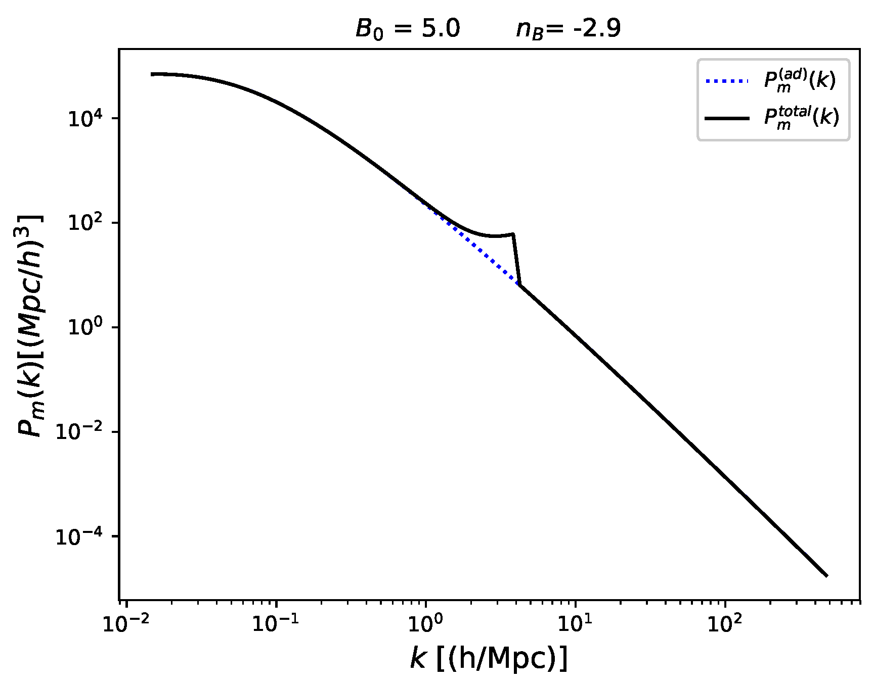
The six-parameter $\mathrm{\Lambda }$CDM model is the minimal bestfit of the observations of the CMB temperature anisotropies and polarization. The density field causing these small fluctuations is described by the adiabatic, primordial curvature mode. This could be produced for example in a standard, slow roll inflationary model. A primordial magnetic field present before decoupling induces different types of cosmological perturbations as well. In linear cosmological perturbation theory there are, in general, three types, namely, scalar, vector and tensor perturbations. All of these are sourced by a primordial magnetic field. However, since here the main focus is on the effect of a magnetic field on the linear matter power spectrum only scalar modes are considered. There are two types of scalar modes caused by a magnetic field. One of them is the passive mode which is of the type of an adiabatic mode but the amplitude is too small to explain the observations and the other is the compensated, pure magnetic mode which is of isocurvature type. Therefore usually it is assumed that there is a dominant adiabatic, primordial curvature mode from inflation, e.g., and a magnetic mode. These two are usually assumed to be uncorrelated at linear level (cf., [18,28]). Moreover, here we assume that the magnetic mode consists only of the compensated magnetic mode. To generate the initial, gaussian matter density the linear matter power spectrum comprising of the standard adiabatic mode and the magnetic mode has been used [24]. As an example, the resulting total linear matter power spectrum for a magnetic field of strength $B=5$ nG and spectral index $n_B=-2.9$ is shown in Figure 1.

Perturbations in a magnetized fluid cannot grow below the magnetic Jeans length as the magnetic pressure counteracts further collapse [29]. This is implemented in a phenomenological way by introducing a sharp cut-off in the linear matter power spectrum at the wave number corresponding to the magnetic Jeans scale $k_J$ given by, $k_J$, [29,30].

$$\begin{array}{c}\hfill \left(\frac{k_J}{{\mathrm{Mpc}}^{-1}}\right)={\left[14.8{\left(\frac{{\mathsf{\Omega }}_m}{0.3}\right)}^{\frac{1}{2}}\left(\frac{h}{0.7}\right){\left(\frac{B}{{10}^{-9}\mathrm{G}}\right)}^{-1}{\left(\frac{k_L}{{\mathrm{Mpc}}^{-1}}\right)}^{\frac{n_B+3}{2}}\right]}^{\frac{2}{n_B+5}}.\end{array}$$

(6)

This sharp cut-off leads to the feature seen in Figure 1. The linear matter power spectrum is normalized to ${\sigma }_8$ of the bestfit parameters of Planck13+WP data [26,27].

The simulations of the 21 cm line signal is done using the semi-analytical code SIMFAST21 [31,32] which is similar to the 21 cmFAST code [33]. The initial Gaussian density field is evolved in time leading to nonlinear structure and formation of dark matter halos. These are identified using the excursion formalism using a minimal, critical value for the amplitude of the density perturbation beyond which a given region is assumed to be undergoing gravitational collapse. Finally using the Zel’dovich approximation corrects the position of the halo position originally based on the linear matter density field. Dark matter halos trace the matter distribution and harbour ionizing sources from first stars and quasars. This allows to determine the distributions of neutral hydrogen which trace the 21 cm line signal. As reionization proceeds regions of 21 cm line emission or absorption disappear.

For the simulations it was assumed for simplicity that the spin temperature is much larger than the temperature of the CMB which is the case if there is heating of matter. There are a number of sources such as heating by UV and X-ray emissions of the first stars and quasars. It could also have more exotic origin such as the annihilation of or decay of dark matter particles. In addition in the case of the presence of large scale magnetic fields there is also heating because of magnetic field diffusion due to the interaction with the cosmic plasma. Close to recombination, magnetic fields are damped by decaying MHD turbulence and in the low redshift universe by plasma drift (also often referred to as ambipolar diffusion) [26,30,34,35]. For $T_S\gg T_{CMB}$ the 21 cm line signal does not depend on $T_S$. The focus of our work in [24] was to study the effect of the modified linear matter power spectrum. Additional heating due to magnetic field dissipation by decaying MHD turbulence and plasma drift are not taken into account.

In [24] simulations have been carried out using the total linear matter power spectrum generated by the primordial curvature mode and the magnetic mode for different choices of the magnetic field parameters. The additional feature in the total linear matter power spectrum on small scales due to the effect of the Lorentz term on the baryon velocity as illustrated in Figure 1 for a magnetic field of strength 5 nG and spectral index $n_B=-2.9$ manifests itself in the linear as well as the non linear density field by an increase of structure on small scales. This is propagated to the distribution of regions of ionized hydrogen as well as the 21 cm line signal. The Square Kilometre Array (SKA) is going to measure the 21 cm line signal. The baseline design of SKA1-LOW is planned to cover a frequency range of 50–350 MHZ [36]. To determine the frequency range which could be of interest to detect the presence of a putative primordial magnetic field the 21 cm line signal has been averaged over the simulation boxes obtained at different redshifts in [24]. In particular, redshifts z between $z=32$ and $z=5$ have been considered in [24]. Taking into account the cosmological redshifting of the frequency this corresponds to a frequency range 1420.4057 MHz/$(1+z)$, that is, 43 MHz and 237 MHz. Using the parameters for the baseline design of SKA1-LOW for an integration time of 1000 h and one beam of bandwidth 300 MHz results in a projected sensitivity which might allow to distinguish between the models under consideration with and without the contribution of the magnetic mode in the linear matter power spectrum observing at frequencies above 120 MHz.

3. Conclusions

Primordial magnetic fields present since before decoupling have a variety of effects on observables, such as as the angular power spectra of the CMB temperature anisotropies and polarization or the linear matter power spectrum. The latter has been the focus of the work [24] reported on at this workshop. The linear matter power spectrum provides the initial conditions for the matter density field which as it evolves to nonlinear structures traces the distribution of neutral hydrogen. The latter being the source or the sink of the 21 cm line signal, respectively. The prospects of observing this signal with SKA has been considered in [24] for magnetic field strengths of 5 nG and spectral indices between −2.9 and −1.5. These values are chosen as way of example. They are of the order of observational constraints obtained from, e.g., the CMB with the Planck 2015 data constraining the magnetic field amplitude to be less than B = 4.4 nG [37]. It has been concluded that there might be a window above frequencies of 120 MHz to distinguish models with and without a magnetic field with the SKA1-LOW baseline design.

References

- Govoni, F.; Murgia, M.; Vacca, V.; Loi, F.; Girardi, M.; Gastaldello, F.; Giovannini, G.; Feretti, L.; Paladino, R.; Carretti, E. Sardinia Radio Telescope observations of Abell 194—The intra-cluster magnetic field power spectrum. Astron. Astrophys. 2017, 603, A122. [Google Scholar] [CrossRef]
- Han, J.L. Observing Interstellar and Intergalactic Magnetic Fields. Ann. Rev. Astron. Astrophys. 2017, 55, 111. [Google Scholar] [CrossRef]
- Beck, R. Magnetic fields in spiral galaxies. Astron. Astrophys. Rev. 2015, 24, 4. [Google Scholar] [CrossRef] [Green Version]
- Arlen, T.; Aune, T.; Beilicke, M.; Benbow, W.; Bouvier, A.; Buckley, J.H.; Bugaev, V.; Byrum, K.; Cannon, A.; Cesarini, A.; et al. Constraints on Cosmic Rays, Magnetic Fields, and Dark Matter from Gamma-Ray Observations of the Coma Cluster of Galaxies with VERITAS and Fermi. Astrophys. J. 2012, 757, 123. [Google Scholar] [CrossRef]
- Feretti, L.; Giovannini, G.; Govoni, F.; Murgia, M. Clusters of galaxies: Observational properties of the diffuse radio emission. Astron. Astrophys. Rev. 2012, 20, 54. [Google Scholar] [CrossRef]
- Bonafede, A.; Feretti, L.; Murgia, M.; Govoni, F.; Giovannini, G.; Dallacasa, D.; Dolag, K.; Taylor, G.B. The Coma cluster magnetic field from Faraday rotation measures. Astron. Astrophys. 2010, 513, A30. [Google Scholar] [CrossRef] [Green Version]
- Clarke, T.E.; Kronberg, P.P.; Boehringer, H. A New radio—X-ray probe of galaxy cluster magnetic fields. Astrophys. J. 2001, 547, L111–L114. [Google Scholar] [CrossRef]
- Takahashi, K.; Mori, M.; Ichiki, K.; Inoue, S.; Takami, H. Lower Bounds on Magnetic Fields in Intergalactic Voids from Long-term GeV-TeV Light Curves of the Blazar Mrk 421. Astrophys. J. 2013, 771, L42. [Google Scholar] [CrossRef]
- Essey, W.; Ando, S.; Kusenko, A. Determination of intergalactic magnetic fields from gamma ray data. Astropart. Phys. 2011, 35, 135–139. [Google Scholar] [CrossRef]
- Tavecchio, F.; Ghisellini, G.; Foschini, L.; Bonnoli, G.; Ghirlanda, G.; Coppi, P. The intergalactic magnetic field constrained by Fermi/LAT observations of the TeV blazar 1ES 0229+200. Mon. Not. R. Astron. Soc. 2010, 406, L70–L74. [Google Scholar] [CrossRef]
- Neronov, A.; Vovk, I. Evidence for strong extragalactic magnetic fields from Fermi observations of TeV blazars. Science 2010, 328, 73–75. [Google Scholar] [CrossRef] [PubMed]
- Boulanger, F.; Ensslin, T.; Fletcher, A.; Girichides, P.; Hackstein, S.; Haverkorn, M.; Hoerandel, J.R.; Jaffe, T.R.; Jasche, J.; Kachelriess, M.; et al. IMAGINE: A comprehensive view of the interstellar medium, Galactic magnetic fields and cosmic rays. arXiv, 2018; arXiv:1805.02496. [Google Scholar] [CrossRef]
- Kandus, A.; Kunze, K.E.; Tsagas, C.G. Primordial magnetogenesis. Phys. Rep. 2011, 505, 1–58. [Google Scholar] [CrossRef] [Green Version]
- Durrer, R.; Neronov, A. Cosmological Magnetic Fields: Their Generation, Evolution and Observation. Astron. Astrophys. Rev. 2013, 21, 62. [Google Scholar] [CrossRef]
- Adamek, J.; Durrer, R.; Fenu, E.; Vonlanthen, M. A large scale coherent magnetic field: Interactions with free streaming particles and limits from the CMB. J. Cosmol. Astropart. Phys. 2011, 1106, 017. [Google Scholar] [CrossRef]
- Barrow, J.D.; Ferreira, P.G.; Silk, J. Constraints on a primordial magnetic field. Phys. Rev. Lett. 1997, 78, 3610–3613. [Google Scholar] [CrossRef]
- Subramanian, K. The origin, evolution and signatures of primordial magnetic fields. Rept. Prog. Phys. 2016, 79, 076901. [Google Scholar] [CrossRef] [Green Version]
- Shaw, J.R.; Lewis, A. Constraining Primordial Magnetism. Phys. Rev. 2012, D86, 043510. [Google Scholar] [CrossRef]
- Brandenburg, A.; Kahniashvili, T.; Mandal, S.; Pol, A.R.; Tevzadze, A.G.; Vachaspati, T. Evolution of hydromagnetic turbulence from the electroweak phase transition. Phys. Rev. 2017, D96, 123528. [Google Scholar] [CrossRef]
- Loeb, A.; Furlanetto, S. The First Galaxies in the Universe; Princeton University Press: Princeton, NJ, USA, 2013. [Google Scholar]
- Mo, H.; van den Bosch, F.; White, S. Galaxy Formation and Evolution; Cambridge University Press: Cambridge, MA, USA, 2010. [Google Scholar]
- Bowman, J.D.; Rogers, A.E.E.; Monsalve, R.A.; Mozdzen, T.J.; Mahesh, N. An absorption profile centred at 78 megahertz in the sky-averaged spectrum. Nature 2018, 555, 67–70. [Google Scholar] [CrossRef]
- Monsalve, R.A.; Fialkov, A.; Bowman, J.D.; Rogers, A.E.E.; Mozdzen, T.J.; Cohen, A.; Barkana, R.; Mahesh, N. Results from EDGES High-Band: III. New Constraints on Parameters of the Early Universe. arXiv, 2019; arXiv:1901.10943. [Google Scholar]
- Kunze, K.E. 21 cm line signal from magnetic modes. J. Cosmol. Astropart. Phys. 2019, 1901, 033. [Google Scholar] [CrossRef]
- Kunze, K.E. Effects of helical magnetic fields on the cosmic microwave background. Phys. Rev. 2012, D85, 083004. [Google Scholar] [CrossRef]
- Kunze, K.E.; Komatsu, E. Constraints on primordial magnetic fields from the optical depth of the cosmic microwave background. J. Cosmol. Astropart. Phys. 2015, 1506, 027. [Google Scholar] [CrossRef]
- Ade, P.A.R.; Aghanim, N.; Armitage-Caplan, C.; Arnaud, M.; Ashdown, M.; Atrio-Barandela, F.; Aumont, J.; Baccigalupi, C.; Banday, A.J.; Barreiro, R.B.; et al. Planck 2013 results. XVI. Cosmological parameters. Astron. Astrophys. 2014, 571, A16. [Google Scholar] [CrossRef]
- Kunze, K.E. CMB anisotropies in the presence of a stochastic magnetic field. Phys. Rev. 2011, D83, 023006. [Google Scholar] [CrossRef]
- Kim, E.j.; Olinto, A.; Rosner, R. Generation of density perturbations by primordial magnetic fields. Astrophys. J. 1996, 468, 28. [Google Scholar] [CrossRef]
- Sethi, S.K.; Subramanian, K. Primordial magnetic fields in the post-recombination era and early reionization. Mon. Not. R. Astron. Soc. 2005, 356, 778–788. [Google Scholar] [CrossRef] [Green Version]
- Santos, M.G.; Ferramacho, L.; Silva, M.B.; Amblard, A.; Cooray, A. Fast and Large Volume Simulations of the 21 cm Signal from the Reionization and pre-Reionization Epochs. Mon. Not. R. Astron. Soc. 2010, 406, 2421–2432. [Google Scholar] [CrossRef]
- Hassan, S.; Dave, R.; Finlator, K.; Santos, M.G. Simulating the 21 cm signal from reionization including non-linear ionizations and inhomogeneous recombinations. Mon. Not. R. Astron. Soc. 2016, 457, 1550–1567. [Google Scholar] [CrossRef] [Green Version]
- Mesinger, A.; Furlanetto, S.; Cen, R. 21cmFAST: A Fast, Semi-Numerical Simulation of the High-Redshift 21-cm Signal. Mon. Not. R. Astron. Soc. 2011, 411, 955. [Google Scholar] [CrossRef]
- Paoletti, D.; Chluba, J.; Finelli, F.; Rubino-Martin, J.A. Improved CMB anisotropy constraints on primordial magnetic fields from the post-recombination ionization history. Mon. Not. R. Astron. Soc. 2018, 484, 185–195. [Google Scholar] [CrossRef]
- Trivedi, P.; Reppin, J.; Chluba, J.; Banerjee, R. Magnetic heating across the cosmological recombination era: Results from 3D MHD simulations. Mon. Not. R. Astron. Soc. 2018, 481, 3401–3422. [Google Scholar] [CrossRef]
- Koopmans, L.V.E.; Pritchard, J.; Mellema, G.; Abdalla, F.; Aguirre, J.; Ahn, K.; Barkana, R.; van Bemmel, I.; Bernardi, G.; Bonaldi, A.; Briggs, F. The Cosmic Dawn and Epoch of Reionization with the Square Kilometre Array. arXiv, 2015; arXiv:1505.07568. [Google Scholar]
- Ade, P.A.R.; Aghanim, N.; Arnaud, M.; Arroja, F.; Ashdown, M.; Aumont, J.; Baccigalupi, C.; Ballardini, M.; Banday, A.J.; Barreiro, R.B.; et al. Planck 2015 results. XIX. Constraints on primordial magnetic fields. Astron. Astrophys. 2016, 594, A19. [Google Scholar] [CrossRef]
Figure 1.
Linear matter power spectrum , including the adiabatic mode and the magnetic mode for a magnetic field of strength nG and spectral index ( solid line). For comparison the pure adiabatic mode has also been included ( dotted line).
© 2019 by the author. Licensee MDPI, Basel, Switzerland. This article is an open access article distributed under the terms and conditions of the Creative Commons Attribution (CC BY) license (http://creativecommons.org/licenses/by/4.0/).
Share and Cite
MDPI and ACS Style
Kunze, K.E. Tracing Primordial Magnetic Fields with 21 cm Line Observations. Galaxies 2019, 7, 37. https://doi.org/10.3390/galaxies7010037
AMA Style
Kunze KE. Tracing Primordial Magnetic Fields with 21 cm Line Observations. Galaxies. 2019; 7(1):37. https://doi.org/10.3390/galaxies7010037
Chicago/Turabian StyleKunze, Kerstin E. 2019. "Tracing Primordial Magnetic Fields with 21 cm Line Observations" Galaxies 7, no. 1: 37. https://doi.org/10.3390/galaxies7010037
Note that from the first issue of 2016, this journal uses article numbers instead of page numbers. See further details here.