The Laboratory Astrophysics Spectroscopy Programme at Imperial College London
by
María Teresa Belmonte
*, 
Juliet C. Pickering
,
Christian P. Clear
,
Florence Concepción Mairey
and
Florence Liggins
Blackett Laboratory, Imperial College London, London SW7 2AZ, UK
*
Author to whom correspondence should be addressed.
Galaxies 2018, 6(4), 109; https://doi.org/10.3390/galaxies6040109
Submission received: 2 August 2018
/
Revised: 2 October 2018
/
Accepted: 9 October 2018
/
Published: 13 October 2018
(This article belongs to the Special Issue Atomic and Molecular Data Needs for Astronomy and Astrophysics)
Abstract
:Accurate atomic parameters, such as transition probabilities, wavelengths, and energy levels, are indispensable for the analysis of stellar spectra and the obtainment of chemical abundances. However, the quantity and quality of the existing data in many cases lie far from the current needs of astronomers, creating an acute need for laboratory measurements of matching accuracy and completeness to exploit the full potential of the very expensively acquired astrophysical spectra. The Fourier Transform Spectrometer at Imperial College London works in the vacuum ultraviolet-visible region with a resolution of 2,000,000 at 200 nm. We can acquire calibrated spectra of neutral, singly, and doubly ionized species. We collaborate with the National Institute of Standards and Technology (NIST) and the University of Lund to extend our measurements into the infrared region. The aim of this review is to explain the current capabilities of our experiment in an understandable way to bring the astronomy community closer to the field of laboratory astrophysics and encourage further dialogue between our laboratory and all those astronomers who need accurate atomic data. This exchange of ideas will help us to focus our efforts on the most urgently needed data.
1. Introduction
The Fourier Transform Spectrometer (FTS) Laboratory at Imperial College London has been working on the measurement of atomic and molecular parameters for the last 30 years. A remarkable growth in the capabilities of ground- and space-based instrumentation has pushed the field of astronomy to a point where very accurate atomic data is needed to exploit the immense capability of current Galactic Surveys. The lack of accurate wavelengths, energy levels, and transition probabilities for many of the most common elements found in stellar spectra and the poor quality of existing data call for a collective effort to take place.
Our experience of attending conferences within the field of astronomy has led us to believe that the main difficulties in establishing successful and efficient collaborations between data users (astronomers) and data producers (either experimental or theoretical) are a lack of a common language and an absence of a good understanding of the other fields. On the one hand, data producers struggle to gain a clear idea of the most urgently needed data, whereas, on the other hand, astronomers struggle to grasp what can be done in terms of experimental measurement and what the capabilities of the different laboratories working in the field are. Experience has shown us that this lack of mutual understanding can be very easily solved in many cases if the main concepts and ideas from each field are explained to non-experts in a clear and simple way.
The aims of this contribution are to address the main ideas underlying the measurement of atomic parameters (wavelengths, energy levels, transition probabilities, hyperfine and isotope structure constants) for all those data users (especially astronomers) who are not familiar with the field, and to explain the capabilities of our laboratory. An understanding of the strengths and limitations of our instrument will help to establish further successful collaborations with astronomers in need of atomic and molecular data. We also provide a summary of the latest work carried out by our group in collaboration with other institutions and descriptions of our current and future projects.
There are several review papers concerning laboratory astrophysics which focus on the Fourier spectroscopy technique [1,2], data needed [3,4], the latest results in the field, and projects undertaken by the main groups within it [5,6]. Very detailed and clear descriptions of the need for atomic and molecular data within the field of astronomy can be found in Allende Prieto (2016) [7] and Barklem (2016) [8]. The aim of this paper, rather than to present an exhaustive account of data needs or recent results, is to bring non-experts closer to the field of laboratory astrophysics and the capabilities and practices of our laboratory. In terms of atomic parameters, we will focus most closely on the measurement of transition probabilities (log(gf) values) given their importance and the recent review of atomic data for wavelengths and energy levels by Nave et al. (2017) [5].
2. Our Experimental Set-Up
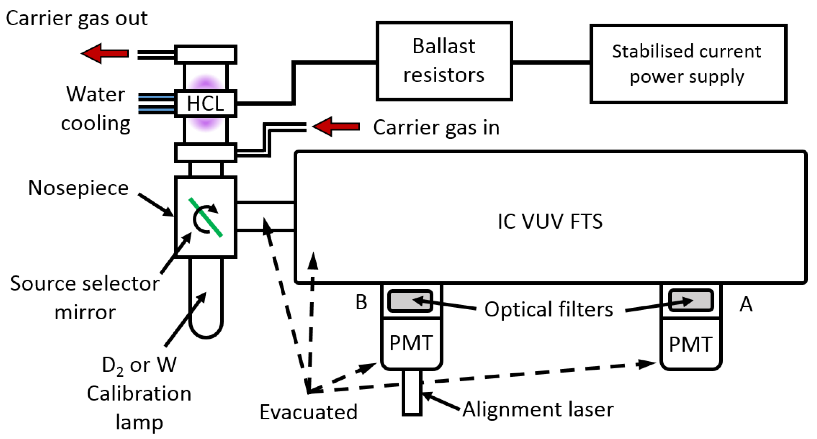
Astronomers record radiation coming from stars, which are their given “problem” light sources, and then analyse its spectral composition (using known atomic data) to obtain information about the elements these stars are made of. The opposite process is done in the laboratory, where we analyse the light emitted by a source of our choice (with a known chemical composition) to obtain the unknown atomic parameters. A diagram of our experimental set-up is shown in Figure 1.
Generally, we use matter in plasma state as a light source. This plasma is generated inside a lamp, which can be either commercial or made in-house. The advantage of the latter is that they are far more versatile as they can be run at different currents and be filled with different gases to obtain the spectral lines of interest. Currents and gas pressure conditions are carefully optimized to obtain the highest signal-to-noise ratio (SNR) for the lines we are interested in (especially the weakest ones) while avoiding self-absorption (the phenomenon by which part of the radiation emitted is reabsorbed by the same plasma before leaving the lamp, causing changes to the profile and strength of the spectral lines observed and therefore distorting the measurement of both wavelengths and transition probabilities). Commercial lamps tend to run at low currents which, on many occasions, are insufficient to offer lines from high-lying energy levels. We use two different customised lamps: a water-cooled Hollow Cathode Lamp (HCL), made at Imperial College, to produce lines of neutral and singly ionised elements (Figure 2); and a Penning discharge lamp made at the University of Hannover, for doubly ionised elements. These lamps are chosen as they run very stably.
Once we have solved the problem of generating the radiation, we need to extract the information about the different wavelengths present in it. To do that, one could use either a dispersive element, such as a prism or a diffraction grating, or an interferometric technique (combined with Fourier analysis). This last method, known as Fourier Transform Spectroscopy, is that used in our laboratory. A detailed description of this technique can be found in [2,10]. It is important to note the main advantages of Fourier Transform Spectroscopy, which are:
- Combination of high resolution and wide wavelength range
- Linear wavenumber scale
- Slowly varying intensity response function
Finally, we use a photomultiplier tube (PMT) detector appropriate for the spectral region of interest to record an interferogram which contains information about the intensity at all the wavelengths. Several interferograms are normally recorded and co-added to improve the SNR before we Fourier transform them using the XGREMLIN package [11] to obtain the final spectrum. A comparison of an FTS and a grating recorded spectrum is shown in Figure 3.
Spectra need to be wavelength and intensity calibrated. For wavelength calibration, we use a set of Ar II lines [13] measured by Whaling et al. (1995) [14]. For the intensity calibration, we use two standard intensity calibrated lamps to obtain the response function of our spectrometer in the VUV-visible spectral range. For the region ranging from 140 to 350 nm, we use a deuterium lamp (D2) calibrated by the Physikalisch-Technische Bundesanstalt (PTB) in Germany. Above 300 nm, we use a tungsten lamp (W) calibrated by the UK National Physical Laboratory (NPL).
Once calibrated, spectral lines are generally fitted with Voigt profiles (a centre-of-gravity fitting is used when hyperfine and isotopic structure or blends are present). The fitting of the spectral lines provides three key quantities: the central wavelength of the spectral line, the full width at half maximum (FWHM), and the total area under the profile, which is known as the relative intensity of the line. The main characteristics of our instrument are summarized in Table 1.
3. Our Laboratory Measurements
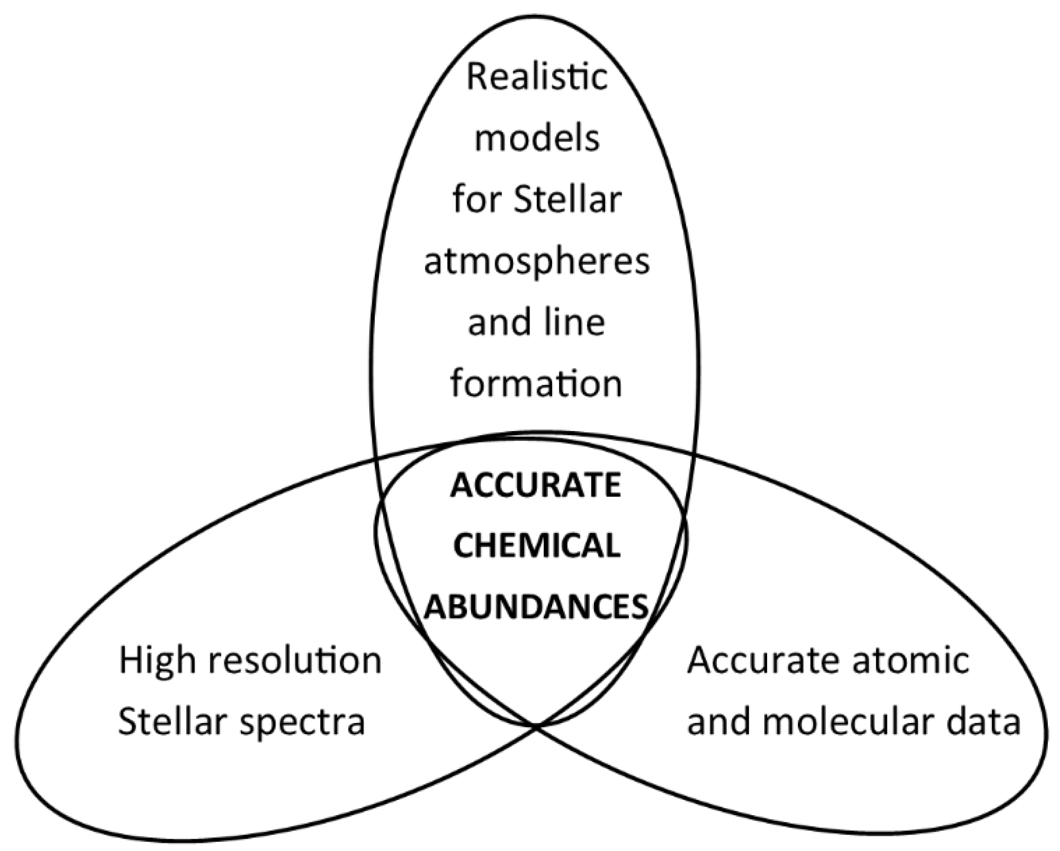
Quantitative interpretation of stellar spectra relies on the existence and accuracy of atomic data such as wavelengths, transition probabilities, energy levels, and hyperfine structure constants. Well-defined linelists with reliable and consistent atomic data are also very important for the analysis of deviations from local thermodynamic equilibrium (non-LTE effects) when modelling stellar atmospheres [15,16,17,18]. Together with realistic stellar models and high-resolution stellar spectra, accurate atomic and molecular data are essential to obtain chemical abundances with the level of accuracy needed by Galactic Surveys (Figure 4). Our laboratory provides high quality experimental data for all these purposes from recorded high-resolution laboratory spectra.
3.1. Transition Probabilities
Transition probabilities or oscillator strengths (f-values, log(gf) values) are essential for the analysis of stellar spectra as they relate to the intensity of the different spectral lines used to obtain abundances of different elements. Several approaches can be used to obtain these parameters. Laboratory measurements, theoretical calculations, and reverse solar analysis [19] are the most common, with each of them presenting both advantages and disadvantages.
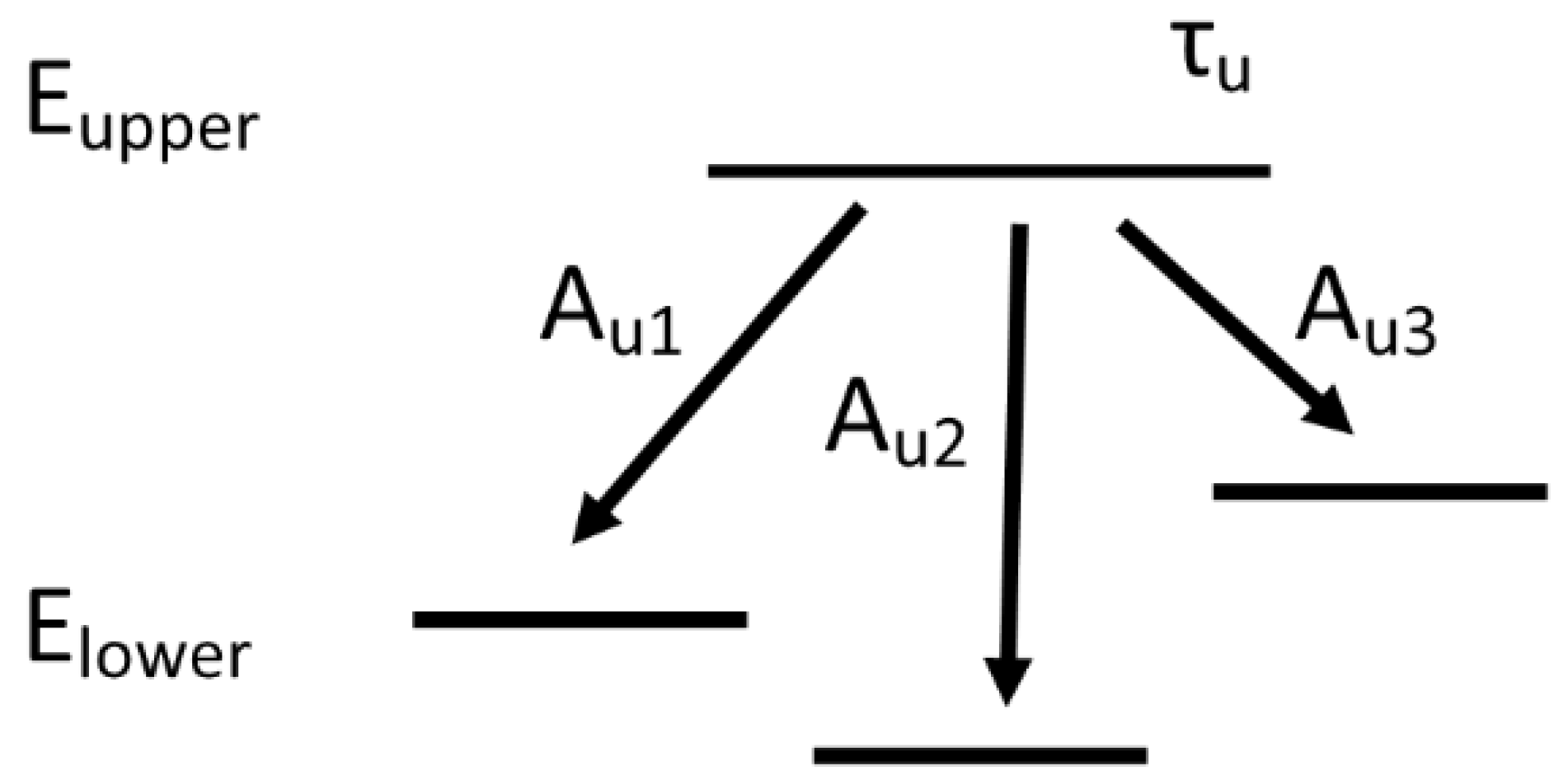
If we consider an atom or ion in an excited state, there are different possible channels by which the electron in an upper energy level can decay to a lower one, as shown in Figure 5. Each of these possible transitions can be characterized by its Einstein coefficient for spontaneous emission, Aul, also known as the transition probability.
The mean lifetime, τu, of that upper energy level is defined as the time in which the population of that level, Nu(t), decays to 1/e of its initial value and can be expressed as a function of the transition probabilities for every possible transition:
The “intensity” of a spectral line, Iul, understood as the total number of photons involved in a particular transition and taking into account that a spectral line is not a Dirac delta function, but a Voigt profile around the central wavelength due to the different broadening mechanisms, can be experimentally obtained as the area under the fitted spectral line profile. From the theoretical point of view, we can express the intensity of a spectral line as [20,21]:
where Aul is the transition probability and Nu is the population of the upper energy level at a particular instant. Depending on the measurements we are carrying out, we can play with this expression in different ways [22], bearing in mind that the intensity of the line (area under the fitted spectral line) is the quantity we can measure in the laboratory with FTS and the Aul is the parameter we normally want to obtain. Regarding the remaining quantity (the population of the upper energy level) two approaches can be followed depending on the kind of light source used and the characteristics of the experiment:
Boltzmann-Plottechnique: If the plasma used as a light source is known to be in at least local thermodynamic equilibrium (LTE), the population of the upper energy level will follow a Boltzmann distribution and expression (2) can be rewritten as:
where N0 is the total number density of the species considered, gu is the degeneracy of the upper energy level, Z(T) is the partition function, kB is the Boltzmann constant, and T is the temperature of the plasma. Several methods can be used to obtain the plasma temperature. A very good review of them can be found in Table 1 from Wiese (1991) [20]. If the transition probabilities of some lines are well known, the plasma temperature can be obtained by using the so-called Boltzmann plot or slope technique [21]. The transition probabilities used to determine the plasma temperature are the “normalizing” factor and establish the absolute scale of the measurements. This technique is useful in obtaining large sets of data and when lifetimes for certain energy levels are not available or cannot be measured. A recent example of this technique can be found in Nitz et al. (2018) [23]. The main problems of this method are the assumption of equilibrium and the need for some pre-measured data of good quality.
These two problems can be avoided with the technique used in our laboratory, the branching fraction method.
Branchingfraction technique: This ingenious approach [24,25] removes the necessity of having to consider the population of the upper energy level (which depends on the plasma thermodynamic state) by looking at all the transitions coming from a given upper energy level. Firstly, for convenience, we define the so-called branching fraction, BF, as [24]:
This branching fraction can be obtained by measuring relative line intensities from the recorded intensity calibrated spectra. As we are considering spectral lines all coming from the same upper energy level, we can see from Equation (2) how the intensity of a line only depends on the transition probability in a linear way, allowing us to rewrite (4) as:
Making use of Equations (1) and (5), we can express the transition probability as:
We can therefore obtain experimental values of transition probabilities combining BF and lifetimes. Firstly, we identify all the lines coming from the upper energy level of interest using semi-empirical calculations from Kurucz [26]. These calculations are also used to estimate the contribution from missing lines due to them being too weak to be observed, blended, or outside the observed wavelength range [27]. In most cases, the fraction α of the total intensity that is missing is less than 5% and a correction factor (1 + α) is applied to in Equation (4) to account for these missing lines. We use Equation (4) to determine branching fractions from line intensities measured in our laboratory, as explained in Section 2, which are then combined with the lifetime of the upper energy level to get transition probabilities.
Lifetimes can be measured with time-resolved laser-induced fluorescence (TRLIF) [28,29] or beam foil techniques [25], or obtained from theoretically calculated values. The main challenges of this method are the need to measure all the significant transitions coming from the upper energy level of interest (even if those spectral lines can lie very far apart in terms of wavelength) and the necessity of the upper energy level lifetime, which sets the absolute scale in this case (as the Aul does in the previous method).
The branching fraction method, combined with TRLIF measurements of lifetimes, has been extensively used by our laboratory in collaboration with NIST (USA) and the Universities of Lund (Sweden) and Wisconsin (USA) to obtain transition probabilities, which are converted into oscillator strengths, f, and usually into the log(gf) required by astronomers using the expression [25]:
where gl and gu are the statistical weights of the lower and upper energy levels, respectively, and λ is the wavelength of the line expressed in nm.
We provide log(gf) values of neutral and singly ionized atoms with uncertainties as low as 0.02 dex (5%) for strong lines, and are currently focusing on iron-group elements due to the great demand for these by astronomers. A very significant effort has been made to obtain accurate transition probabilities of Fe I, both in the infrared (IR) [30] and in the visible-UV region [31,32,33], due to its importance in different Galactic surveys such as APOGEE [34] and Gaia-ESO [35]. Table 2 includes a list of the publications of log(gf) values in which our laboratory has participated in the last 15 years. The third column includes the total number of log(gf) values provided in each work, with the number of values for which previous measurements did not exist between parentheses. The uncertainty of the measured log(gf) values varies from line to line, so we provide a range (in dex, with x dex = 10x) in the fourth column.
One of the key aspects in the determination of transition probabilities is the estimation of the uncertainty, which helps data users (astronomers) and groups creating databases and linelists for their use in astronomy (VALD [40], VAMDC [41], BRASS [42], Gaia-ESO [43], APOGEE [44]) to decide which values should be included, especially when more than one data set is available. Very detailed descriptions regarding all the possible sources of uncertainty that should be taken into account (depending on the experimental method used to obtain Aul) can be found in [45,46,47]. As can be seen from Equation (8) [48], the uncertainty of the chemical abundances is directly proportional to that of the oscillator strength, f:
where EW is the equivalent width of the spectral lines from stellar spectra. This supports the importance of improving the quality of these atomic parameters. Our determination of uncertainties, which follows the expression suggested in Sikstrom et al., (2002) [49], is explained in detail in [30]. We consider the uncertainties coming from the intensity calibration, the signal-to-noise ratio of the line, and the uncertainty of the lifetime. In those cases where more than one spectrum is needed to include all the lines coming from a given upper energy level, the resulting additional uncertainty is incorporated [27,50]. The method described in Sikstrom et al., (2002) [49] considers isolated and well-defined spectral lines. It is also possible to include the effect of partial blends, the presence of nearby lines, and self-absorption on the accuracy with which the area of a line is determined (and therefore, the transition probability), as done in [51].
In the case of theoretical transition probabilities, the determination of the intrinsic uncertainties is more complicated due to the complexity of the methods used [21]. However, it is possible to develop some indicators of the quality of calculated data, as explained in Hibbert (2018) [52], or use methods such as that of Kramida (2014) [53]. Comparisons with experimental data are also essential to validate new theoretical calculations. Alternatives for experimental lifetimes need to be found for the IR region, where many of the energy level lifetimes required are not accessible to time-resolved laser-induced fluorescence (TRLIF). This is due to the fact that spectral lines in this region come from relatively highly excited energy levels, which are difficult to populate in a LIF experiment. A possible solution to this problem is to use synthetic and observed stellar spectra to obtain “astrophysical” parameters, as done in Ruffoni et al., (2013) [30].
3.2. Wavelengths, Energy Levels, Hyperfine and Isotopic Structure
Our laboratory has a long tradition in the measurement of wavelengths, energy levels, and hyperfine structure constants, particularly for iron group elements. A good overview of these measurements can be found in Nave et al., (2017) [5]. There are several ongoing analyses of atomic spectra at the moment, including Mn II, Ni II, Mn I, and Fe III.
These very lengthy studies generally improve the accuracy of wavelengths and energy levels by at least an order of magnitude with respect to the previously published data, when available. The uncertainty in the wavelength of the spectral lines recorded with the FTS varies depending on the wavelength region and the SNR of the line. For lines observed with high SNR, the uncertainty of the calibration plays a fundamental role, whereas for weak lines, the statistical uncertainty is dominant. As a rough guide, the wavenumber of strong lines in the VUV can be measured with accuracies of 0.001 cm−1, where this improves to up to 0.0005 cm−1 for strong IR lines.
Due to the high resolution of FTS spectra, we can resolve and study the hyperfine and isotope structures of spectral lines, which are vital for the correct identification of lines in stellar spectra. Figure 6 shows an example of the isotopic structure of a Ni II spectral line. Examples of measured lines with a hyperfine structure can be found in [36,54].
4. Future Work and Collaborations
Our group continues to work with established collaborations, such as APOGEE, for which much work remains to be done in the IR, not only for elements like Fe, but also in neutron-capture elements. We are also working actively to establish new collaborations and would like to encourage all those groups with specific needs to contact us. We have recently joined the WEAVE consortium [55] and will work actively towards the development of a defined list of anticipated needs. Table 3 provides an overview of the main Galactic Surveys, both ongoing and in development, with an interest in obtaining chemical abundances for different elements, which are normally:
- Light proton-capture elements: Li, C, O
- α-elements: Mg, Si, Ca, Ti
- Light elements with odd atomic number: Na, Al, K
- Iron-peak elements: Sc, V, Cr, Mn, Fe, Co, Ni, Cu, Zn
- Neutron-capture elements: Rb, Sr,Y, Zr, Ba, La, Ru, Ce, Nd, Eu
The total number of elements whose chemical abundances are investigated in each Survey is included in the fifth column of Table 3, with the aimed uncertainty in their abundance between parentheses.
One of the main problems when establishing collaborations between data providers and astronomers is a lack of information about the data needed. Astronomers working closely with stellar spectra have a much more accurate feeling for the data that is missing, as sometimes only a few spectral lines of an element are being used to obtain chemical abundances. It is then very important that astronomers define a clear and concise list of priorities. With such a list as a starting point, data producers can examine how feasible or time-consuming obtaining the needed values will be and arrange the submitted list accordingly. Interaction of this type between astronomers and data producers is key to optimizing the use of time. Important efforts are being made by astronomers to publish papers which include details of the spectral lines used and which subsequently point towards which data are missing. This practice is incalculably helpful to data producers as it draws attention to current outstanding needs for data improvement.
Finally, it is worth mentioning several challenges faced by the laboratory astrophysics community. The most pressing amongst these is insufficient funding for researchers given the duration of some projects. Full analyses of atomic spectra, for example, can easily demand a time span of several years. This underfunding also delays the extremely useful critical compilation of atomic data, work traditionally carried out at NIST, which is increasingly in demand from and appreciated by data users who lack the experience necessary to adequately evaluate the quality of the different data sets. A recent example of this kind of work can be found in [58]. The other major problem in the field is a lack of citations of the work carried out by experimentalists, especially when considering the time scale of these projects. Very important efforts are being made by those involved in the development of databases (such as VAMDC) to make sure that the work of data producers is acknowledged in the publications where this data is used [59]. We would like to actively encourage astronomers to include references to original sources when using atomic and molecular data. We understand that this process can be very tedious when using values from many different authors, but acknowledgement of this work is the only way of supporting the effort of data producers as they attempt to secure funding with which to keep the laboratories in operation.
5. Conclusions
The Fourier Transform Spectroscopy Laboratory at Imperial College London has been providing accurate atomic data (wavelengths, transition probabilities, energy levels, and hyperfine structure constants), often in collaboration with the National Institute of Standards and Technology (USA) and the Universities of Lund (Sweden) and Wisconsin (USA), over the last three decades. Our group has a long history of collaboration with astronomers, who constitute the main data users. Astronomers provide us with very valuable feedback on our newly measured data, having used it to produce synthetic spectra for comparison with high quality stellar spectra of benchmark stars; a contrastive process which allows for the identification of inconsistencies.
To meet the rapidly increasing data needs of astronomers, driven by new telescopes and surveys, an active interaction and exchange of ideas between the astronomy community and that of data producers is necessary. To establish long-term productive collaborations, we understand that it is essential to develop a common language and nurture a good understanding of the basic ideas in both fields. This contribution aims to provide non-experts with a broad and basic understanding of experimental laboratory astrophysics and of the current capabilities of our laboratory.
We would also like to launch an appeal to collaborate with all those astronomers who need accurate atomic data and encourage further dialogue regarding the most pressing data needs, as this will help us to focus our efforts on the most urgently needed data.
Author Contributions
Investigation, M.T.B., J.C.P., C.P.C., F.C.M., and F.L.; Writing-Original Draft Preparation, M.T.B.; Writing-Review & Editing, J.C.P. and M.T.B.; Funding Acquisition, J.C.P.
Funding
This research was funded by STFC of UK.
Conflicts of Interest
The authors declare no conflict of interest.
References
- Pickering, J.C. Laboratory Astrophysics: Improving the Atomic Data by Fourier Transform Spectrometry. Phys. Scr. 1999, T83, 27–34. [Google Scholar] [CrossRef]
- Pickering, J.C. High resolution Fourier transform spectroscopy with the Imperial College (IC) UV-FT spectrometer, and its applications to astrophysics and atmospheric physics: A review. Vib. Spectrosc. 2002, 29, 27–43. [Google Scholar] [CrossRef]
- Pickering, J.C.; Blackwell-Whitehead, R.; Thorne, A.P.; Ruffoni, M.P.; Holmes, C.E. Laboratory measurements of oscillator strengths and their astrophysical applications. Can. J. Phys. 2011, 89, 387–393. [Google Scholar] [CrossRef]
- Wahlgren, G.M. Atomic data for stellar astrophysics: From the UV to the IR. Can. J. Phys. 2011, 89, 345–356. [Google Scholar] [CrossRef]
- Nave, G.; Sansonetti, C.J.; Townley-smith, K.; Pickering, J.C.; Thorne, A.P.; Liggins, F.; Clear, C. Comprehensive atomic wavelengths, energy levels, and hyperfine structure for singly ionized iron-group elements. Can. J. Phys. 2017, 816, 811–816. [Google Scholar] [CrossRef]
- Lawler, J.E.; Sneden, C.; Cowan, J.J.; Den Hartog, E.A.; Wood, M.P. Laboratory transition probabilities for studies of nucleosynthesis of Fe-group elements. Can. J. Phys. 2017, 10, 783–789. [Google Scholar] [CrossRef]
- Allende Prieto, C. Solar and stellar photospheric abundances. Living Rev. Sol. Phys. 2016, 13, 1–40. [Google Scholar] [CrossRef]
- Barklem, P.S. Accurate abundance analysis of late-type stars: advances in atomic physics. Astron. Astrophys. Rev. 2016, 24, 1–54. [Google Scholar] [CrossRef]
- Clear, C.P. The Spectrum and Term Analysis of Singly Ionised Nickel. Ph.D. Thesis, Imperial College London, London, UK, 2018. [Google Scholar]
- Davis, S.P.; Abrams, M.C.; Brault, J.W. Fourier Transform Spectrometry; Academic Press: Cambridge, MA, USA, 2001. [Google Scholar]
- Nave, G.; Griesmann, U.; Brault, J.W.; Abrams, M.C. XGREMLIN: Interferograms and spectra from Fourier transform spectrometers analysis, Astrophysics Source Code Library, record ascl:1511.004, 2015. Available online: https://github.com/gnave/Xgremlin (accessed on 12 October 2018).
- Smillie, D.G.; Pickering, J.C.; Nave, G.; Smith, P.L. The spectrum and term analysis of Co III measured using Fourier Transform and grating spectroscopy. Astrophys. J. Suppl. Ser. 2016, 223, 12. [Google Scholar] [CrossRef]
- Learner, R.C.M.; Thorne, A.P. Wavelength calibration of Fourier-transform emission spectra with applications to Fe I. J. Opt. Soc. Am. B 1988, 5, 2045–2059. [Google Scholar] [CrossRef]
- Whaling, W.; Anderson, W.H.C.; Carle, M.T.; Brault, J.W.; Zarem, H.A. Argon ion linelist and level energies in the hollow-cathode discharge. J. Quant. Spectrosc. Radiat. Transf. 1995, 53, 1–22. [Google Scholar] [CrossRef]
- Amarsi, A.M.; Lind, K.; Asplund, M.; Barklem, P.S.; Collet, R. Non-LTE line formation of Fe in late-type stars - III. 3D non-LTE analysis of metal-poor stars. Mon. Not. R. Astron. Soc. 2016, 463, 1518–1533. [Google Scholar] [CrossRef]
- Lind, K.; Amarsi, A.M.; Asplund, M.; Barklem, P.S.; Bautista, M.; Bergemann, M.; Collet, R.; Kiselman, D.; Leenaarts, J.; Pereira, T.M.D. Non-LTE line formation of Fe in late-type stars- IV. Modelling of the solar centre-to-limb variation in 3D. Mon. Not. R. Astron. Soc. 2017, 4322, 4311–4322. [Google Scholar] [CrossRef]
- Bergemann, M.; Collet, R.; Schoenrich, R.; Andrae, R.; Kovalev, M.; Ruchti, G.; Hansen, C.J.; Magic, Z. Non-local thermodynamic equilibrium stellar spectroscopy with 1D and 3D models - II. Chemical properties of the Galactic metal-poor disk and the halo. Astrophys. J. 2016, 847, 16. [Google Scholar] [CrossRef]
- Bergemann, M.; Collet, R.; Amarsi, A.M.; Kovalev, M.; Ruchti, G.; Magic, Z. Non-local thermodynamic equilibrium stellar spectroscopy with 1D and 3D models—I. Methods and application to magnesium abundances in standard stars. Astrophys. J. 2017, 847, 15. [Google Scholar] [CrossRef]
- Borrero, J.M.; Rubio, L.R.B.; Barklem, P.S.; Iniesta, J.C.T. Accurate atomic parameters for near-infrared spectral lines. Astron. Astrophys. 2003, 404, 749–762. [Google Scholar] [CrossRef] [Green Version]
- Wiese, W.L. Spectroscopic diagnostics of low temperature plasmas: techniques and required data. Spectrochim. Acta Part B At. Spectrosc. 1991, 46, 831–841. [Google Scholar] [CrossRef]
- Wiese, W.L. Atomic Oscillator Strengths for Light Elements–Progress and Problems. J. Korean Phys. Soc. 1998, 33, 207–213. [Google Scholar]
- Musielok, J.; Wiese, W.L.; Veres, G. Atomic transition probabilities and tests of the spectroscopic coupling scheme for N I. Phys. Rev. A 1995, 51, 3588–3597. [Google Scholar] [CrossRef] [PubMed]
- Nitz, D.E.; Curry, J.J.; Buuck, M.; Demann, A.; Mitchell, N.; Shull, W. Transition probabilities of Ce I obtained from Boltzmann analysis of visible and near-infrared emission spectra. J. Phys. B At. Mol. Opt. Phys. 2018, 51, 045007. [Google Scholar] [CrossRef] [Green Version]
- Huber, M.C.E.; Sandeman, R.J. The measurement of oscillator strengths. Reports Prog. Phys. 1986, 49, 397–490. [Google Scholar] [CrossRef]
- Thorne, A.P.; Litzén, U.; Johansson, S. Spectrophysics; Springer: Berlin, Germany, 1999; ISBN 3-540-65117-9. [Google Scholar]
- Kurucz, R.L. Kurucz Database. Available online: http://kurucz.harvard.edu/atoms.html (accessed on 12 October 2018).
- Pickering, J.C.; Thorne, A.P.; Perez, R. Oscillator strengths of transitions in Ti II in the visible and ultraviolet regions. Astrophys. J. Suppl. Ser. 2001, 132, 403–409. [Google Scholar] [CrossRef]
- Lawler, J.E.; Bergeson, S.D.; Wamsley, R.C. Advanced experimental techniques for measuring oscillator strengths of vacuum ultraviolet lines. Phys. Scr. 1993, 1993, 29–35. [Google Scholar] [CrossRef]
- Pehlivan Rhodin, A.; Belmonte, M.T.; Engström, L.; Lundberg, H.; Nilsson, H.; Hartman, H.; Pickering, J.C.; Clear, C.; Quinet, P.; Fivet, V.; et al. Lifetime measurements and oscillator strengths in singly ionized scandium and the solar abundance of scandium. Mon. Not. R. Astron. Soc. 2017, 472, 3337–3353. [Google Scholar] [CrossRef]
- Ruffoni, M.P.; Allende Prieto, C.; Nave, G.; Pickering, J.C. Infrared laboratory oscillator strengths of Fe I in the H-band. Astrophys. J. 2013, 779, 17. [Google Scholar] [CrossRef]
- Ruffoni, M.P.; Den Hartog, E.A.; Lawler, J.E.; Brewer, N.R.; Lind, K.; Nave, G.; Pickering, J.C. Fe I oscillator strengths for the Gaia-ESO survey. Mon. Not. R. Astron. Soc. 2014, 441, 3127–3136. [Google Scholar] [CrossRef]
- Den Hartog, E.A.; Ruffoni, M.P.; Lawler, J.E.; Pickering, J.C.; Lind, K.; Brewer, N.R. Fe I oscillator strengths for transitions from high-lying even-parity levels. Astrophys. J. Suppl. Ser. 2014, 215, 23. [Google Scholar] [CrossRef]
- Belmonte, M.T.; Pickering, J.C.; Ruffoni, M.P.; Den Hartog, E.A.; Lawler, J.E.; Guzman, A.; Heiter, U. Fe I Oscillator Strengths for Transitions from High-lying Odd-parity Levels. Astrophys. J. 2017, 848, 125. [Google Scholar] [CrossRef]
- Majewski, S.R.; Schiavon, R.P.; Frinchaboy, P.M.; et al. The Apache Point Observatory Galactic Evolution Experiment (APOGEE). Astron. J. 2017, 154, 94. [Google Scholar] [CrossRef] [Green Version]
- Gilmore, G.; Randich, S.; Asplund, M.; Binney, J.; Bonifacio, P.; Drew, J.; Feltzing, S.; Ferguson, A.; Jeffries, R.; Micela, G.; et al. The Gaia-ESO Public Spectroscopic Survey. Messenger 2012, 147, 25–31. [Google Scholar]
- Holmes, C.E.; Pickering, J.C.; Ruffoni, M.P.; Blackwell-Whitehead, R.; Nilsson, H.; Engström, L.; Hartman, H.; Lundberg, H.; Belmonte, M.T. Experimentally Measured Radiative Lifetimes and Oscillator Strengths in Neutral Vanadium. Astrophys. J. Suppl. Ser. 2016, 224, 35. [Google Scholar] [CrossRef]
- Lyubchik, Y.; Jones, H.R.A.; Pavlenko, Y.V.; Viti, S.; Pickering, J.C.; Blackwell-Whitehead, R.J. Atomic lines in infrared spectra for ultracool dwarfs. Astron. Astrophys. 2004, 416, 655–659. [Google Scholar] [CrossRef] [Green Version]
- Blackwell-Whitehead, R.J.; Lundberg, H.; Nave, G.; Pickering, J.C.; Jones, H.R.A.; Lyubchik, Y.; Pavlenko, Y.V.; Viti, S. Experimental Ti i oscillator strengths and their application to cool star analysis. Mon. Not. R. Astron. Soc. 2006, 373, 1603–1609. [Google Scholar] [CrossRef]
- Blackwell-Whitehead, R.J.; Xu, H.L.; Pickering, J.C.; Nave, G.; Lundberg, H. Experimental oscillator strengths for the spectrum of neutral manganese. Mon. Not. R. Astron. Soc. 2005, 361, 1281–1286. [Google Scholar] [CrossRef] [Green Version]
- Ryabchikova, T.; Piskunov, N.; Kurucz, R.L.; Stempels, H.C.; Heiter, U.; Pakhomov, Y.; Barklem, P.S. A major upgrade of the VALD database. Phys. Scr. 2015, 90, 054005. [Google Scholar] [CrossRef]
- Dubernet, M.L.; Antony, B.K.; Ba, Y.A.; Babikov, Y.L.; Bartschat, K.; Boudon, V.; Braams, B.J.; Chung, H.-K.; Daniel, F.; Delahaye, F.; et al. The virtual atomic and molecular data centre (VAMDC) consortium. J. Phys. B At. Mol. Opt. Phys. 2016, 49, 074003. [Google Scholar] [CrossRef] [Green Version]
- Laverick, M.; Lobel, A.; Merle, T.; Royer, P.; Martayan, C.; David, M.; Hensberge, H.; Thienpont, E. The Belgian repository of fundamental atomic data and stellar spectra (BRASS). I. Cross-matching atomic databases of astrophysical interest. Astron. Astrophys. 2018, 612, A60. [Google Scholar] [CrossRef]
- Heiter, U.; Lind, K.; Asplund, M.; Barklem, P.S.; Bergemann, M.; Magrini, L.; Masseron, T.; Mikolaitis; Pickering, J.C.; Ruffoni, M.P. Atomic and molecular data for optical stellar spectroscopy. Phys. Scr. 2015, 90, 054010. [Google Scholar] [CrossRef] [Green Version]
- Shetrone, M.; Bizyaev, D.; Lawler, J.E.; Prieto, C.A.; Johnson, J.A.; Smith, V.V.; Cunha, K.; Holtzman, J.; García Pérez, A.E.; Mészáros, S.Z.; et al. The SDSS-III apogee spectral line list for H-Band spectroscopy. Astrophys. J. Suppl. Ser. 2015, 221, 24. [Google Scholar] [CrossRef]
- Vujnović, V.; Wiese, W.L. A Critical Compilation of Atomic Transition Probabilities for Singly Ionized Argon. J. Phys. Chem. Ref. Data 1992, 21, 919–939. [Google Scholar] [CrossRef]
- Wiese, W.L. The Critical Assessment of Atomic Oscillator Strengths. Phys. Scr. 1996, T65, 188–191. [Google Scholar] [CrossRef]
- Taylor, B.N.; Kuyatt, C.E. Guidelines for Evaluating and Expressing the Uncertainty of NIST Measurement Results. NIST Tech. Note 1994, 1297. Available online: http://citeseerx.ist.psu.edu/viewdoc/download?doi=10.1.1.437.5767&rep=rep1&type=pdf (accessed on 20 December 2018).
- Pehlivan Rhodin, A. Experimental and Computational Atomic Spectroscopy for Astrophysics: Oscillator Strengths and Lifetimes for Mg I, Si I, Si II, Sc I and Sc II. Ph.D. Thesis, Lund University, Lund, Sweden, March 2018. [Google Scholar]
- Sikstrom, C.M.; Nilsson, H.; Litzen, U.; Blom, A.; Lundberg, H. Uncertainty of oscillator strengths derived from lifetimes and branching fractions. J. Quant. Spectrosc. Radiat. Transf. 2002, 74, 355–368. [Google Scholar] [CrossRef]
- Pickering, J.C.; Johansson, S.; Smith, P.L. The FERRUM project: Branching ratios and atomic transition probabilities of Fe II transitions from the 3d6(a3F)4p subconfiguration in the visible to VUV spectral region. Astron. Astrophys. 2001, 337, 361–367. [Google Scholar] [CrossRef]
- Belmonte, M.T.; Djurovic, S.; Pelaez, R.J.; Aparicio, J.A.; Mar, S. Improved and expanded measurements of transition probabilities in UV Ar II spectral lines. Mon. Not. R. Astron. Soc. 2014, 445, 3345–3351. [Google Scholar] [CrossRef] [Green Version]
- Hibbert, A. Successes and Difficulties in Calculating Atomic Oscillator Strengths and Transition Rates. Galaxies 2018, 6, 77. [Google Scholar] [CrossRef]
- Kramida, A. Assessing Uncertainties of Theoretical Atomic Transition Probabilities with Monte Carlo Random Trials. Atoms 2014, 2, 86–122. [Google Scholar] [CrossRef] [PubMed]
- Bergemann, M.; Pickering, J.C.; Gehren, T. NLTE analysis of Co I/Co II lines in spectra of cool stars with new laboratory hyperfine splitting constants. Mon. Not. R. Astron. Soc. 2010, 401, 1334–1346. [Google Scholar] [CrossRef]
- Dalton, G.; Trager, S.; Abrams, D.C.; Bonifacio, P.; Aguerri, J.A.L.; Middleton, K.; Benn, C.; Dee, K.; Sayède, F.; Lewis, I.; et al. Final design and progress of WEAVE: the next generation wide-field spectroscopy facility for the William Herschel Telescope. Proc. SPIE Ground-Based Airborne Instrum. Astron. VI 2016, 9908, 99081G. [Google Scholar] [CrossRef]
- Martell, S.L.; Sharma, S.; Buder, S.; Duong, L.; Schlesinger, K.J.; Simpson, J.; Lind, K.; Ness, M.; Marshall, J.P.; Asplund, M.; et al. The GALAH survey: Observational overview and Gaia DR1 companion. Mon. Not. R. Astron. Soc. 2017, 465, 3203–3219. [Google Scholar] [CrossRef]
- Jong, R.S. de; 4MOST Consortium. Complementing asteroseismology with 4MOST spectroscopy. Astron. Nachr. 2016, 337, 964–969. [Google Scholar] [CrossRef]
- Cashman, F.H.; Kulkarni, V.P.; Kisielius, R.; Ferland, G.J.; Bogdanovich, P. Atomic Data Revisions for Transitions Relevant to Observations of Interstellar, Circumgalactic, and Intergalactic Matter. Astrophys. J. Suppl. Ser. 2017, 230, 8. [Google Scholar] [CrossRef] [Green Version]
- Zwölf, C.M.; Moreau, N.; Dubernet, M.L. New model for datasets citation and extraction reproducibility in VAMDC. J. Mol. Spectrosc. 2016, 327, 122–137. [Google Scholar] [CrossRef] [Green Version]
Figure 1.
Experimental set-up of the Imperial College VUV FTS [9].
Figure 1.
Experimental set-up of the Imperial College VUV FTS [9].

Figure 2.
Photograph of the Hollow Cathode Lamp made at Imperial College London.

Figure 3.
Comparison of FTS (see Table 1) and grating spectra for Co III from Smillie et al., (2016) [12].

Figure 4.
Information needed for accurate chemical abundances.

Figure 5.
Possible decay channels from an upper energy level.

Figure 6.
Experimental and fitted profiles of a non-calibrated Ni II spectral line showing isotopic structure, adapted from [9]. The wavelengths shown are in air.
Figure 6.
Experimental and fitted profiles of a non-calibrated Ni II spectral line showing isotopic structure, adapted from [9]. The wavelengths shown are in air.


Table 1.
Main characteristics of the VUV-Visible FTS at Imperial College London.
| Spectral range | 140–800 nm |
| Max. path difference | 20 cm |
| Resolving power | 2,000,000 at 200 nm |
| Min resolution limit | 0.025 cm−1 at 50,000 cm−1 |
| Max free spectral range | 64,000 cm−1 |
| Beamsplitter | Magnesium fluoride |
| Detector | Photomultiplier tube (PMT) |
| Dimensions | 1.5 × 0.25 × 0.25 m |
Table 2.
Log(gf) measurements taken with the participation of our laboratory in the last 15 years.
| Element | Spectral Range | Total Log(gf) (New) | Uncert (Dex) | Reference |
|---|---|---|---|---|
| Fe I | 213–1033 nm | 120 (22) | 0.02–0.1 | Belmonte et al., (2017) [33] |
| Sc II | 158–425 nm | 57 (57) | 0.03–0.11 | Pehlivan et al., (2017) [29] |
| V I | 304–2000 nm | 208 (13) | 0.02–0.1 | Holmes et al., (2016) [36] |
| Fe I | 320–1102 nm | 203 (81) | 0.02–0.11 | Den Hartog et al., (2014) [32] |
| Fe I | 352–1087 nm | 142 (64) | 0.02–0.14 | Ruffoni et al., (2014) [31] |
| Fe I | 1.5–1.7 µm | 28 (28) | 0.05–0.11 | Ruffoni et al., (2013) [30] |
| Mn I | 321–1400 nm | 20 (15) | 0.02–0.05 | Blackwell-Whitehead et al., (2011) [37] |
| Ti I | 465–3892 nm | 88 (67) | 0.04–0.08 | Blackwell-Whitehead et al., (2006) [38] |
| Mn I | 209–2780 nm | 44 (24) | 0.03–0.1 | Blackwell-Whitehead et al., (2005) [39] |
Table 3.
Overview of some of the main Galactic Surveys, both ongoing and in development.
| Survey [ref.] | Instrument | Spectral Region | Resolving Power | Number Elements (Uncert Dex) | Date |
|---|---|---|---|---|---|
| APOGEE [34] | APOGEE | 1.51–1.7 µm | ~22,500 | 15 (0.1) | Ongoing |
| Gaia-ESO [35] | FLAMES-GIRAFFE | 400–480 nm | 16,200– | >~20 | Ongoing |
| 510–560 nm | 25,900 | ||||
| 630–680 nm | |||||
| 850–900 nm | |||||
| FLAMES-UVES | 410–680 nm | 47,000 | |||
| GALAH [56] | HERMES | 471.8–490.3 nm 564.9–587.3 nm 648.1–673.9 nm 759.0–789.0 nm | 28,000 (50,000) | 30 (0.05) | Ongoing |
| WEAVE [55] | WEAVE | 366–959 nm | 5000 20,000 | 2019 | |
| 4MOST [57] | HRS | 392.6–436.5 nm 516–573.8 nm 612–681 nm | >18,000 | 15 | 2021 |
© 2018 by the authors. Licensee MDPI, Basel, Switzerland. This article is an open access article distributed under the terms and conditions of the Creative Commons Attribution (CC BY) license (http://creativecommons.org/licenses/by/4.0/).
Share and Cite
MDPI and ACS Style
Belmonte, M.T.; Pickering, J.C.; Clear, C.P.; Concepción Mairey, F.; Liggins, F. The Laboratory Astrophysics Spectroscopy Programme at Imperial College London. Galaxies 2018, 6, 109. https://doi.org/10.3390/galaxies6040109
AMA Style
Belmonte MT, Pickering JC, Clear CP, Concepción Mairey F, Liggins F. The Laboratory Astrophysics Spectroscopy Programme at Imperial College London. Galaxies. 2018; 6(4):109. https://doi.org/10.3390/galaxies6040109
Chicago/Turabian StyleBelmonte, María Teresa, Juliet C. Pickering, Christian P. Clear, Florence Concepción Mairey, and Florence Liggins. 2018. "The Laboratory Astrophysics Spectroscopy Programme at Imperial College London" Galaxies 6, no. 4: 109. https://doi.org/10.3390/galaxies6040109
Note that from the first issue of 2016, this journal uses article numbers instead of page numbers. See further details here.