Prediction of Soluble Al2O3 in Calcined Kaolin Using Infrared Spectroscopy and Multivariate Calibration


Resource Engineering Section, Department of Geoscience and Engineering, Delft University of Technology, Stevinweg 1, 2628 CN Delft, The Netherlands
*
Author to whom correspondence should be addressed.
Minerals 2018, 8(4), 136; https://doi.org/10.3390/min8040136
Submission received: 9 March 2018
/
Revised: 25 March 2018
/
Accepted: 26 March 2018
/
Published: 28 March 2018
Abstract
:In the production of calcined kaolin, the soluble Al2O3 content is used as a quality control criterion for some speciality applications. The increasing need for automated quality control systems in the industry has brought the necessity of developing techniques that provide (near) real-time data. Based on the understanding that the presence of water in the calcined kaolin detected using infrared spectroscopy can be used as a proxy for the soluble Al2O3 measurement, in this study, a hand-held infrared spectrometer was used to analyse a set of calcined kaolin samples obtained from a production plant. The spectra were used to predict the amount of soluble Al2O3 in the samples by implementing partial least squares regression (PLS-R) and support vector regression (SVR) as multivariate calibration methods. The presence of non-linearities in the dataset and the different types of association between water and the calcined kaolin represented the main challenges for developing a good calibration. In general, SVR showed a better performance than PLS-R, with root mean squared error of the cross-validation (RMSECV) and for the best-achieved prediction. This accuracy level is adequate for detecting variation trends in the production of calcined kaolin which could be used not only as a quality control strategy, but also for the optimisation of the calcination process.
1. Introduction
High-grade kaolin is mainly composed of the mineral kaolinite [Al2Si2O5(OH)4], and is commonly thermally treated for industrial purposes [1]. This process aims to tailor the physical and chemical properties of the original mineral to specific market specifications. When kaolinite is calcined to high temperatures (above 600 ), it dehydroxylates and transforms into amorphous metakaolinite [Al2Si2O7] (Equation (1)), which has typically high chemical reactivity. Calcination to temperatures around 980 transforms the metakaolinite into the spinel phase (Al-spinel [Al2O3] and Si-spinel [SiO2]) (Equation (2)), followed by the nucleation of the spinel and transformation into mullite (Equation (3)), which is characteristically hard and abrasive [2,3,4].
For applications in the pharmaceutical industry, natural kaolin is calcined to temperatures around 1100 in industrial furnaces to generate a product in an intermediate stage between the amorphous and crystalline spinel phase. This stage marks the balance point between low reactivity and low abrasiveness that is required for calcined kaolin products [5]. In the industry, the criterion to assess the extent of the calcination reaction is the chemical extraction of soluble Al2O3. This method makes use of the solubility of the alumina in the spinel phase (-alumina) in strong acids [6,7,8] to estimate the reactivity of the calcined kaolin [9,10]. Consequently, the extraction of soluble Al2O3 is employed as the standard operational procedure (SOP) to determine the quality of the calcined product. However, this is a laboratory and time-consuming method that restricts timely operational feedback, thus limiting the opportunities for the on-line optimisation of the calcination process.
The development of an on-site and (near) real-time method that can support the SOP and can be used as an on-site quality control measurement would benefit the production of calcined kaolin [11]. Other researchers have developed different strategies for controlling the extent of the calcination process inside a multiple hearth furnace (MHF). For example, Thomas et al. [5] investigated the residence time of kaolin in the calciner to improve the consistency of the properties of the calcined product; Eskelinen et al. [12] modelled some of the furnace’s variables and related them to the physical-chemical phenomena taking place during calcination. However, these studies did not address a mechanism for quality control of the calcined product directly. Recently, Guatame-Garcia et al. [13] investigated the relationship between the infrared spectra of the kaolin calcination reaction and the changes in the calcined clay’s reactivity, measured as soluble Al2O3. Infrared spectroscopy is particularly useful in the characterisation of the kaolin calcination reactions. The spectral features describe changes in the mineral structure related to the kaolinite dehydroxylation (Equation (1)) and recrystallisation of the spinel and mullite phases (Equations (2) and (3)) [14,15,16]. Besides these transformations, the results reported by [13] showed an inverse correlation between the adsorption of water by the calcined clay as detected by the water-related spectral features, and the soluble Al2O3 content. Since the spectral ranges that exhibit the spectrum of water can be measured by using portable and hand-held spectrometers, infrared spectroscopy could be used as an on-site and (near) real-time proxy for the SOP.
To be able to correlate the spectra of calcined kaolin samples—and in particular the water-related spectral features—with the soluble Al2O3 content and establish quantitative predictions for unknown samples, it is necessary to use a chemometric approach [17]. Chemometrics has been used, for example, in applications for mineral processing and control of zinc [18], coal [19,20], and petroleum oil [21]. The correlation between spectral data and the mineral characteristics is commonly done by using multivariate calibration methods, among which partial least squares regression (PLS-R) [22] is often used as the standard methodology. However, in the presence of non-linearities or complex datasets, it is not possible to implement PLS-R. In these cases, multivariate non-linear models such as support vector regression (SVR) should be used along with spectral processing strategies [23,24]. SVR models operate in a kernel-induced feature space that facilitates non-linear modelling with a good performance, even for relatively small datasets, leading to more robust and accurate predictions [21,25]. The use of PLS-R and SVR calibrations can generate a method for the quantification and prediction of soluble Al2O3 in calcined kaolin products based on their infrared spectra.
In this study, spectral processing strategies such as standard normal variate (SNV) and continuum removal (CR), combined with PLS-R and SVR regression are applied on the infrared spectra of calcined kaolin samples to determine their soluble Al2O3 content. Different combinations of spectral processing strategies and model calibration parameters are tested on the spectral regions that exhibit water features. The performance of the generated models is compared and discussed in the view of the use of an infrared-based prediction model as a quality control strategy in the production of calcined kaolin.
2. Methods
2.1. Calcination of Kaolin and Samples
The samples used in this study were obtained from a kaolin processing plant where natural kaolin is calcined in an industrial multiple hearth furnace (MHF) [12]. The production of calcined kaolin for pharmaceutical applications is performed using the soak calcination method, which involves exposing the kaolin to high temperatures for a prolonged amount of time to guarantee complete calcination. The MHF consists of eight vertical hearths with gas flows as a source of energy. The calcination temperature is controlled by varying the gas flow at determined hearths. The raw kaolin is fed at the top of the first hearth and flows spirally through the furnace moved by rabble arms until it reaches the lowest hearth. Finally, the calcined kaolin is extracted through exit holes at the bottom of the furnace. In the calciner’s operational set-up, the initial and maximum final temperatures are respectively 500 and 1100 , with a residence time of approximately 35 min.
The collected calcined powders are cumulative and homogenised samples taken over a period of 12 h (one shift) after blast-cooling. Since the water content in the samples was one of the critical parameters investigated for analysis, two sampling campaigns were conducted during different seasons to ensure that the possible influence of environmental factors was also considered in the measurements. The first sampling campaign occurred during the summertime under local high precipitation and humidity conditions, whereas the second campaign was carried out in autumn, when the precipitation levels are low. In the first period, only samples from the day shift were collected over 23 consecutive days. In the second period, both day and evening shift samples were collected during 17.5 consecutive days, for a total of 56 samples. Approximately 1 of sample was taken for every shift. Table 1 presents the average chemical composition of the samples.
X-ray diffraction (XRD) analysis was performed to identify the mineral phases that can influence the infrared spectra. The XRD patterns were collected with a Bruker D8 Advance diffractometer (PANalytical, Almelo, The Netherlands) featuring Bragg Brentano geometry using a Cu-K radiation of 45 kV and 40 mA on powders placed on a PMMA holder L25. The XRD spectra were measured with a coupled scan ranging from 10 to 110 2 (step size: 2, time per step: 1 s ). The XRD patterns displayed in Figure 1 show that the calcined kaolin is mostly amorphous, with crystalline phases related to illite and quartz. Diffraction peaks characteristic of Al-spinel (-alumina) and mullite are also present.
2.2. Soluble Al2O3
The amount of soluble Al2O3 present in the calcined samples was measured following the conventional method used in the industry, as reported by Taylor [9] and Thomas [10]. The extraction of soluble Al2O3 was done by diluting of sample into 10 of concentrated (16 M) nitric acid (Analar grade) for 4 h. Inductively coupled plasma atomic emission spectroscopy (ICP-AES) determined the concentration of Al2O3 in solution. These analyses were performed at the plant’s laboratory using a Thermo Electron Iris-AP emission spectrometer (TJA Solutions, Windsford, UK); the overall error of the method is reported as .
2.3. Infrared Spectra Collection and Processing
The infrared spectra were collected with an Agilent 4300 hand-held Fourier transform infrared (FTIR) spectrometer (Edinburgh, UK) using a diffuse reflectance interface and coarse silver calibration. The spectra were measured in the range from 5200 to 1250 (1.9 to 8.0 ), with a spectral resolution of 4 and 128 scans per measurement. A petri dish was filled with each of the powder samples; the surface was first compacted and flattened with a spatula to minimise void spaces and then slightly roughened to maximise the direction of the reflections. Five spectral measurements per sample were taken at different spots of the surface. For consistency with previous studies [13], the units were converted from wavenumbers () to wavelengths () during the data import. For every sample, the respective five spectral measurements were averaged as means of noise reduction, generating one spectrum per sample. The resulting spectra were smoothed using the Savitzky–Golay (SG) filter [26] with polynomial order of 3 and windows size of 55 data points. Spectral subsets were made on the regions that exhibit features of molecular water, namely between 2.60 to 3.30 and 5.70 to 6.50 .
The spectral processing strategies used in this study are standard normal variate (SNV) and continuum removal (CR). SNV removes multiplicative interferences caused by scattering and particle size, and corrects shifts in the baseline of the reflectance spectra of powders using a second-degree polynomial regression [27]. CR normalises the albedo of the reflectance curve, which is also known as continuum. It can be modelled as a mathematical function to isolate specific absorption bands [28]. Both signal processing strategies were computed independently for each spectral subset in the R environment using the prospectr package [29].
2.4. Regression Methods
2.4.1. Partial Least Squares Regression
Partial least squares regression (PLS-R) was developed with the aim of maximising the correlation between the information variables and the parameters to be quantified [30]. In regression problems where the variables largely exceed the number of observations, PLS-R decomposes the variables into orthogonal scores and loadings and performs the regression to the scores. The PLS-R latent variables (LVs), which are analogous to the components in principal component analysis (PCA), describe the variability of the input data that is relevant for the determination of the parameters to be predicted [22]. Cross-validation determines the number of LVs that are optimal for the regression. Even though PLS-R is best suited to linear systems, it is also able to cope with mild non-linearities.
For the development of the PLS-R models in this study, the information variables or predictors corresponded to the reflectance value for each wavelength in the infrared spectra, whereas the parameter to be quantified corresponded to the laboratory measurement of soluble Al2O3. In a second experiment, chemical components of the samples (K2O, Fe2O3, and MgO) were also added as input variables. The number of LVs was determined by using 10-fold cross-validation.
2.4.2. Support Vector Regression
Cortes and Vapnik [31] initially established support vector machines (SVMs) to perform binary classification and pattern recognition. After further developments, SVMs have demonstrated to be a powerful technique, particularly in non-linear systems. For solving regression problems, SVMs are implemented via support vector regression (SVR) using the epsilon-insensitive SVR (-SVR) application, which is extensively described in the literature [23,24,32]. -SVR aims to find a function f(x) where the errors or deviations from a target in the training data are not larger than a given value, and that is as flat or smooth as possible. For solving the regression problem, the input data is first mapped into a high dimensional feature space, and kernel functions are used to impart linearity to the dataset. The -SVR function makes use of an -tube that defines the margins where deviations are tolerated; a constant C represents the cost parameter, which determines the trade-off between the flatness of the function and the tolerance in the deviations, assigning greater penalty on the error of the samples outside the -tube. The -insensitive loss function ignores the errors inside the -tube and calculates the loss for the data points outside the -tube based on the distance between the data point and the boundary. All the data points that contribute to the regression are the support vectors (SVs). The analyst should optimise the parameters and C.
For the development of the -SVR models, the input vectors corresponded to the spectra of the samples, and the response vector corresponded to the measured soluble AlO. The -SVR models were developed using the RBF (radial basis function) kernel function. The parameters and C were optimised using a grid search and 10-fold cross-validation.
In this study, for developing the PLS-R and SVR multivariate calibration models, the samples were split into a calibration set (n = 46) and a validation set (n = 10) by random selection. Each spectral subset (2.6 to 3.3 and 5.7 to 6.5 ) was tested under raw, SNV, and CR spectra, for a total of six different test scenarios. All the analyses were performed in the R environment. PLS-R was carried out with the built-in routines in the PLS-R package [33]. For the SVR regression, the interface to LIBSVM [34] in the package e1071 [35] was used. The performance of the models was assessed using the root mean squared error of the cross-validation (RMSECV), the root mean squared error of the calibration (RMSEC), and the root mean squared error of the prediction (RMSEP). The RMSECV corresponds to the results of the 10-fold cross-validation used for the selection of the parameters in the PLS-R and SVR models using the calibration set. The RMSEC was measured as the difference between the predicted and measured soluble Al2O3 values using the calibration set, whereas the RMSEP was measured as the difference between the predicted and measured soluble Al2O3 values using the validation set.
3. Results
The calcined kaolin samples used in this study had soluble Al2O3 content from 0.26 to 0.54 (Table 1). Figure 2 shows that the samples collected in the first period (samples 1 to 23) generally had lower soluble Al2O3 content—average —than those obtained in the second period (samples 24 to 56), with an average of . The variation in the average values between the two periods might reflect differences in the quality of the raw kaolin used as a feed for calcination, volume of material fed into the calciner, or variations in the calciner’s temperature profile. Nevertheless, according to the plant’s historical data, the soluble Al2O3 content in the produced calcined kaolin typically varies from 0.3 to 0.6 . Despite the differences between the two production periods, the sample set covers the production range continuously, ensuring the data representability. These data are the actual values used for developing the calibration PLS-R and SVR models.
3.1. Spectral Processing
The average spectrum of the calcined kaolin clay after SG smoothing is presented in Figure 3. The adsorbed water on the surface of -alumina from the spinel phase exhibits spectral features in two regions. The first region ranges from 2.6 to 3.3 and corresponds to the stretching H–O–H vibrations (); the second region extends from 5.7 to 6.5 , where the O–H bending vibrations () are located [36,37,38]. From the minerals detected by XRD analysis, only illite is expected to have spectral features at 2.74, 3.48 and 5.56 [39]; mullite and quartz are featureless in the presented spectral range. Even though the sample preparation sought to minimise the effect from the environment on the spectra, the CO2 in the air induced artefacts around . The analysis of the spectra of water in -alumina was then constrained to the spectral regions previously described to reduce the influence of the features of illite and CO2.
Figure 4 and Figure 5 display the spectra of the 2.6–3.3 and 6.5–7.5 subsets after Savitzky–Golay (SG) smoothing (hereafter referred to as raw spectra), SNV, and CR processing. In the 2.6 to 3.3 range, spectral processing using SNV and CR (Figure 4b,c) enhances the peak, attributed to the adsorption of water [36]. The other two peaks at 2.73 and 2.75 are also better resolved; however, they can be indistinctly attributed to the presence of water or the surface hydroxyls in illite. The 5.7 to 6.5 region contains only the spectral feature (Figure 5). In this range, SNV and CR processing enhance the depth at the centre of the feature at , apparently separating the spectra into two groups. Besides, the type of spectral processing influences the shape of the spectra. The CR spectra appear to be symmetric, whereas the SNV one is biased towards longer wavelengths, also having a difference in the shoulder position to the deeper spectra at , and that in the shallower one at .
Following the approach proposed in a previous study [13], the depth of the water feature was used to investigate the general behaviour of the spectra of the calcined kaolin samples in relation to the soluble Al2O3 content. Figure 6 shows these parameters using the depth of the feature at extracted from CR spectra. The most remarkable aspect of this plot is that the feature depth separates the samples collected in the first and the second period. The samples of the first period—which have the lowest soluble Al2O3—have a deep water feature, whereas in samples of the second period (with higher soluble Al2O3), this feature is shallower, as was expected from former studies. However, in an individual assessment of every period, it is difficult to describe a pattern of correlation between the depth of the water feature and the soluble Al2O3 content. A proper assessment of the spectral features of water in relation to the amount of soluble Al2O3 in calcined kaolin samples should include not only the depth, but also the overall shape of the spectral feature. Besides, the clustering of data points in Figure 6 and lack of trends make it clear that the relationship between the spectra and the soluble Al2O3 is not linear. As a consequence, a multivariate approach that can cope with non-linearities is more appropriate than a univariate one.
3.2. Multivariate Calibration
Table 2 presents the results of the PLS-R models developed for the six scenarios by using only the infrared spectra as the information variables. In general, the difference in the performance of the models is minimal. Since the RMSECV for all the scenarios is in principle the same, the selection of the best model was based on the lowest RMSEC and RMSEP, which is the model generated from the 5.7 to 6.5 SNV processed spectra, using two LVs and with a prediction error . For this model, the coefficient of determination is . The measured vs. predicted plot (Figure 7a) shows clustering rather than an even distribution along the regression line. The same is true for the predicted values from the validation set. In addition, the residuals plot (Figure 7b) shows large residuals—particularly for the extremes, where low and high values have respectively strong negative and positive residuals. These results suggest that in this case, the PLS-R calibration is not able to cope entirely with the non-linearity of the dataset.
A possible cause of the non-linearity might be related to the mineralogical content of the samples. The interpretation of the XRD and infrared spectra revealed that the samples also contain illite. Even though the relative amount of illite is low, its presence can contribute to the variability of the spectra. In order to consider the influence of illite in the performance of the PLS-R calibration, the chemical contents associated exclusively to illite—i.e., K2O, Fe2O3, and MgO—were included as information variables. The results of the calibration for the six scenarios are presented in Table 3. Compared to the previous results, when taking illite into account, the performance indicators of the new models are slightly better. Moreover, in the measured vs. predicted plot (Figure 8a), the data points are more evenly distributed along the regression line than those presented in Figure 7, suggesting that the inclusion of illite as a variable can improve the performance of the model. However, Figure 8 also shows a poor prediction for high soluble Al2O3 values and larger residuals for some data points, leading to a low coefficient of determination (). Even though the consideration of illite seems to correct for the non-linearities in the dataset, the overall result of the calibration is not optimal.
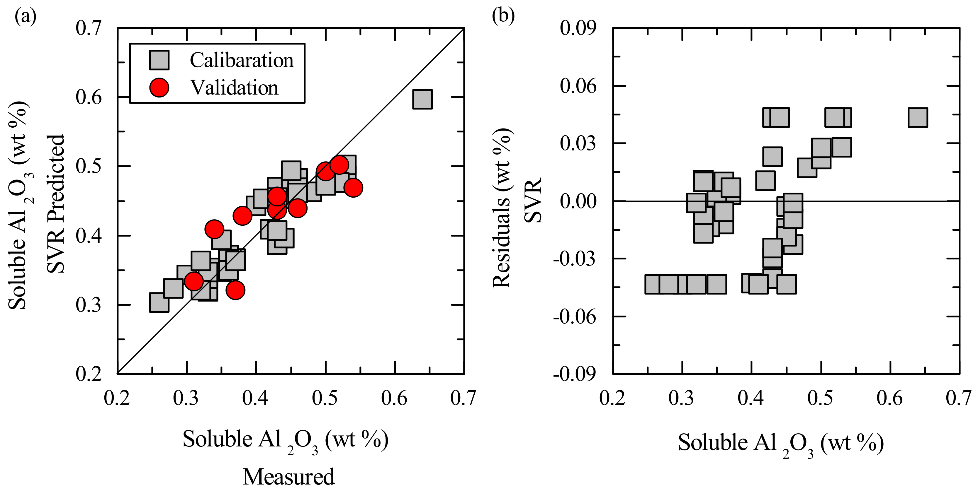
Another strategy for coping with non-linearities is the implementation of SVR models. The results of the SVR calibration for the six scenarios are presented in Table 4. The SVR cross-validation errors do not differ significantly from those reported by the PLS-R models; however, the RMSECs of the SVR are considerably smaller than the PLS-R ones, indicating better performance. The performance of the SVR models improved after applying spectral processing; however, the most notorious improvement occurred in the 5.7 to 6.5 spectra using CR ( ), which was consequently selected as the best model. The coefficient of determination for this model is , which confirms its good performance. The measured vs. predicted plot (Figure 9a) shows that even though the data points seem to separate into two groups, there is an even distribution along the regression line for the entire dataset. Moreover, the predicted values from the validation set are also evenly distributed, except for the values above . The magnitude of the residuals (Figure 9b) is remarkably smaller than those of the best PLS-R model; however, their spread shows that the low values are generally over-estimated, whereas the highest values are under-estimated.
4. Discussion
Prior studies noted the correlation between the reactivity of calcined kaolin and the hydration of -alumina when the calcination reaches the spinel phase. Such a relationship was also assessed by the amount of extracted soluble Al2O3 and the infrared spectral features of water adsorbed by -alumina in the calcined clay. In this study, infrared spectroscopy was used to determine the soluble Al2O3 content in the calcined clay utilising a combination of spectral processing strategies and multivariate calibration. Even though previous studies suggested that the depth of the water spectral features could predict the soluble Al2O3 content, the results of this work showed that such direct prediction is not possible. Since the depth of the water feature captures not only the water physically adsorbed on the surface of -alumina but also all the water present in the system (i.e., chemically bound and free water), the depth parameter is influenced by the -alumina properties as well as the sample’s environmental conditions. In Figure 6, the separation of the two sampling periods by the water parameter indicates differences in the total amount of water present in the samples, where those with a larger exposure to water from the environment have the deepest features. Therefore, the proper assessment of the relationship between soluble Al2O3 and adsorbed water requires the analysis of the water the features as a whole in such a way that the spectral characteristics that relate to physically adsorbed water would have more relevance than those that are related to chemically bound or free water.
Since the spectral analysis must take the shape of the water feature into account, it is relevant to select an appropriate spectra processing strategy. The main difference between the strategies used in this study is that CR exaggerates the spectral features for a more precise discrimination. As a consequence, CR processing enhances the depth differences in the spectra of the water feature, thus increasing variations that are not relevant to the calibration. Using CR in the PLS-R modelling influenced the number of LVs required for the prediction, making only one or two LVs necessary for achieving a low prediction error. However, the calibration assigns high loadings to the peak of the feature enhancing the influence of the feature’s depth, hindering a good prediction. Consequently, the RMSEC of the calibrations using CR-processed spectra were consistently larger than those processed with SNV, given that SNV assigned relatively small loadings to the feature’s depth. In contrast, for the SVR modelling, the performances of the calibrations generated from CR spectra are better than those from SNV. The SVs used in these models seem to reduce the influence of the depth differences, although they are not eliminated, while giving more importance to features that are related to water adsorption.
Aside from the spectral processing, the selection of a spectral range also influenced the performance of the multivariate calibrations. In general, the errors of the models in the 2.6 to 3.3 range are higher than those in the 5.7 to 6.5 . Even though both ranges represent water features related to water adsorption, the presence of illite produces a mixed spectrum around that explains the underperformance of the calibrations. Since the feature in the 5.7 to 6.5 range is exclusive for water, the calibrations in this part of the spectrum are more reliable. However, illite itself can also host water, inducing error to the predictions. The results of the PLS-R calibrations that included the chemical components of illite as variables show that there is indeed an influence of this mineral in the performance of the predictions. However, the inclusion of these variables can make the models more sensitive to errors induced by other types of impurities. To achieve more reliable calibrations, it would be necessary to quantify the amount of illite in the calcined clay and estimate its actual influence on the spectra.
Overall, the performance indicators in all the assessed scenarios indicate that the SVR calibrations are more accurate than the PLS-R ones. However, the most evident difference in the performance between SVR and PLS-R models is shown by the residuals of the different achieved models. The size and the distribution of the PLS-R residuals are evidence of a poor calibration, and suggest that a non-linear approach should be used. The smaller SVR residuals indicate a better calibration; however, the model struggles with the high and low values by systematically over-estimating values lower than and under-estimating values higher than . As a consequence, a note of caution is due here for the interpretation of new predictions that result in values lower than or higher than , since they might be considered as over-calcination in the first case, and under-calcination in the latter.
Even though the accuracy of the model with the best performance (5.7 to 6.5 spectra after CR processing) which has an is lower than the one of the SOP ( ), it is enough for detecting variations in the soluble Al2O3 content in the calcined clay. For this sort of application, the lower performance of the prediction at extreme values—i.e., around and —is not of great consequence, since the over- or under-predicted values are still an indication of general variation trends in the calcination output. These factors encourage the use of the SVR predictions based on infrared spectra as part of a control system.
For an on-site and (near) real-time implementation scenario, the fact that the prediction model is based on spectra collected with a hand-held instrument increases the likelihood that such a system can be used in a mineral production environment. Moreover, the delimitation of the spectral range that is useful for the prediction optimises the required time for spectral collection and data processing. This approach enables the analysis of a larger volume of material than the one that could be possibly measured by the SOP. Therefore, the predicted soluble Al2O3 values could assist a more efficient utilisation of the SOP by performing the laboratory analysis in specifically determined samples. Furthermore, the infrared-based predicted values for soluble Al2O3 could be used to support the in-plant monitoring by improving operational feedback, thus making an impact on the performance of the calciner and the quality of the calcined product.
5. Conclusions
Soluble Al2O3, as an industrial parameter for quality control in calcination, is related to the formation of -alumina and consequently to the reactivity of the calcined clay. In the infrared spectra, the presence of -alumina is evidenced by the spectral features related to water adsorption. However, the nature of the water spectra (which captures not only adsorbed but also chemically bound and free water) hinders a univariate or linear relation with the amount of soluble Al2O3.
This study developed multivariate calibration models for the prediction of the content of soluble Al2O3 in calcined kaolin clays by using infrared spectroscopy. A combination of factors that affect the achievement of a good prediction was used to develop testing scenarios: (1) spectral regions where the water features are present between 2.6 to 3.3 and 5.7 to 6.5 ; (2) standard normal variate (SNV) and continuum removal (CR) as spectral processing strategies to improve the discrimination among the different forms in which water is present in the samples; (3) partial least squares regression (PLS-R) and support vector regression (SVR) as multivariate calibration methods that cope with non-linearity.
In general, the SVR models demonstrated a better ability to relate the water features to the soluble Al2O3 parameter than the PLS-R ones. The best-performing model was achieved by using SVR in the 5.7 to 6.5 range after CR processing. The SVR model predicts the soluble Al2O3 content in the calcined clay with and . Even though this level of accuracy is lower than that one of the standard operational procedure (SOP), it is suitable for detecting variation trends in the production of calcined kaolin. These results encourage the use of infrared spectroscopy as a technique for (near) real-time quality control that supports the optimisation of the calcination process.
Acknowledgments
The authors wish to thank IMERYS Ltd., UK for the access to the samples. This work has been financially supported by the European FP7 project “Sustainable Technologies for Calcined Industrial Minerals in Europe” (STOICISM), grant NMP2-LA-2012-310645 and the EIT Raw Materials KAVA funding “Integrated system for Monitoring and Control of Product quality and flexible energy delivery in Calcination” (MONICALC), grant 15045.
Author Contributions
A.G.-G. and M.B. conceived and designed the experiments; A.G.-G. performed the experiments analysed the data; A.G.-G. wrote the paper and M.B. reviewed it before submission.
Conflicts of Interest
The authors declare no conflict of interest. The founding sponsors had no role in the design of the study; in the collection, analyses, or interpretation of data; in the writing of the manuscript, and in the decision to publish the results.
References
- Murray, H.H. Chapter 5 Kaolin Applications. Dev. Clay Sci. 2006, 2, 85–109. [Google Scholar]
- Gualtieri, A.; Bellotto, M. Modelling the structure of the metastable phases in the reaction sequence kaolinite-mullite by X-ray scattering experiments. Phys. Chem. Miner. 1998, 25, 442–452. [Google Scholar] [CrossRef]
- Chakraborty, A.K. New Data on Thermal Effects of Kaolinite in the High temperature Region. J. Therm. Anal. Calorim. 2003, 71, 799–808. [Google Scholar] [CrossRef]
- Ptáček, P.; Šoukal, F.; Opravil, T.; Nosková, M.; Havlica, J.; Brandštetr, J. Mid-infrared spectroscopic study of crystallization of cubic spinel phase from metakaolin. J. Solid State Chem. 2011, 184, 2661–2667. [Google Scholar] [CrossRef]
- Thomas, R.; Grose, D.; Obaje, G.; Taylor, R.; Rowson, N.; Blackburn, S. Residence time investigation of a multiple hearth kiln using mineral tracers. Chem. Eng. Process. Process Intensif. 2009, 48, 950–954. [Google Scholar] [CrossRef]
- Hulbert, S.F.; Huff, D.E. Kinetics of alumina removal from a calcined kaolin with nitric, sulphuric and hydrochloric acids. Clay Miner. 1970, 8, 337–345. [Google Scholar] [CrossRef]
- Phillips, C.; Wills, K. A laboratory study of the extraction of alumina of smelter grade from China clay micaceous residues by a nitric acid route. Hydrometallurgy 1982, 9, 15–28. [Google Scholar] [CrossRef]
- Ruiz-Santaquiteria, C.; Skibsted, J. Reactivity of Heated Kaolinite from a Combination of Solid State NMR and Chemical Methods. In RILEM Bookseries; Springer: Amsterdam, The Netherlands, 2015; pp. 125–132. [Google Scholar]
- Taylor, R.J. Treatment of Metakaolin. United Kingdom WO2005108295 A1, 17 November 2005. [Google Scholar]
- Thomas, R. High Temperature Processing of Kaolinitic Materials. Ph.D. Thesis, University of Birmingham, Birmingham, UK, 2010. [Google Scholar]
- Glass, H.J. Geometallurgy—Driving Innovation in the Mining Value Chain. In Proceedings of the Third AusIMM International Geometallurgy Conference (GeoMet) 2016, Perth, Australia, 15–17 June 2016; The Australasian Institute of Mining and Metallurgy: Melbourne, Australia, 2016; pp. 21–28. [Google Scholar]
- Eskelinen, A.; Zakharov, A.; Jämsä-Jounela, S.L.; Hearle, J. Dynamic modeling of a multiple hearth furnace for kaolin calcination. AIChE J. 2015, 61, 3683–3698. [Google Scholar] [CrossRef]
- Guatame-García, A.; Buxton, M.; Deon, F.; Lievens, C.; Hecker, C. Towards an On-line Characterisation of Kaolin Calcination Process Using Short-Wave Infrared Spectroscopy. Miner. Process. Extr. Metall. Rev. 2018, in press. [Google Scholar]
- Percival, H.J.; Duncan, J.F.; Foster, P.K. Interpretation of the Kaolinite-Mullite Reaction Sequence from Infrared Absorption Spectra. J. Am. Ceram. Soc. 1974, 57, 57–61. [Google Scholar] [CrossRef]
- Frost, R.L.; Makó, E.; Kristóf, J.; Kloprogge, J.T. Modification of kaolinite surfaces through mechanochemical treatment—A mid-IR and near-IR spectroscopic study. Spectrochim. Acta Part A Mol. Biomol. Spectrosc. 2002, 58, 2849–2859. [Google Scholar] [CrossRef]
- Drits, V.A.; Derkowski, A.; Sakharov, B.A.; Zviagina, B.B. Experimental evidence of the formation of intermediate phases during transition of kaolinite into metakaolinite. Am. Mineral. 2016, 101, 2331–2346. [Google Scholar] [CrossRef]
- Chryssikos, G.; Gates, W. Spectral Manipulation and Introduction to Multivariate Analysis. Dev. Clay Sci. 2017, 8, 64–106. [Google Scholar]
- Haavisto, O.; Hyötyniemi, H. Recursive multimodel partial least squares estimation of mineral flotation slurry contents using optical reflectance spectra. Anal. Chim. Acta 2009, 642, 102–109. [Google Scholar] [CrossRef] [PubMed]
- Andrés, J.; Bona, M. Analysis of coal by diffuse reflectance near-infrared spectroscopy. Anal. Chim. Acta 2005, 535, 123–132. [Google Scholar] [CrossRef]
- Bona, M.; Andrés, J. Coal analysis by diffuse reflectance near-infrared spectroscopy: Hierarchical cluster and linear discriminant analysis. Talanta 2007, 72, 1423–1431. [Google Scholar] [CrossRef] [PubMed]
- Filgueiras, P.R.; Sad, C.M.; Loureiro, A.R.; Santos, M.F.; Castro, E.V.; Dias, J.C.; Poppi, R.J. Determination of API gravity, kinematic viscosity and water content in petroleum by ATR-FTIR spectroscopy and multivariate calibration. Fuel 2014, 116, 123–130. [Google Scholar] [CrossRef]
- Wold, S.; Sjöström, M.; Eriksson, L. PLS-regression: a basic tool of chemometrics. Chemom. Intell. Lab. Syst. 2001, 58, 109–130. [Google Scholar] [CrossRef]
- Devos, O.; Ruckebusch, C.; Durand, A.; Duponchel, L.; Huvenne, J.P. Support vector machines (SVM) in near infrared (NIR) spectroscopy: Focus on parameters optimization and model interpretation. Chemom. Intell. Lab. Syst. 2009, 96, 27–33. [Google Scholar] [CrossRef]
- Li, H.; Liang, Y.; Xu, Q. Support vector machines and its applications in chemistry. Chemom. Intell. Lab. Syst. 2009, 95, 188–198. [Google Scholar] [CrossRef]
- Brereton, R.G.; Lloyd, G.R. Support Vector Machines for classification and regression. Analyst 2010, 135, 230–267. [Google Scholar] [CrossRef] [PubMed]
- Savitzky, A.; Golay, M.J.E. Smoothing and Differentiation of Data by Simplified Least Squares Procedures. Anal. Chem. 1964, 36, 1627–1639. [Google Scholar] [CrossRef]
- Barnes, R.J.; Dhanoa, M.S.; Lister, S.J. Standard Normal Variate Transformation and De-Trending of Near-Infrared Diffuse Reflectance Spectra. Appl. Spectrosc. 1989, 43, 772–777. [Google Scholar] [CrossRef]
- Clark, R.N.; Roush, T.L. Reflectance spectroscopy: Quantitative analysis techniques for remote sensing applications. J. Geophys. Res. 1984, 89, 6329–6340. [Google Scholar] [CrossRef]
- Stevens, A.; Ramirez-Lopez, L. An introduction to the prospectr package. In R Package Vignette; R Foundation for Statistical Computing; Vienna, Austria, 2014. [Google Scholar]
- Höskuldsson, A. PLS regression methods. J. Chemom. 1988, 2, 211–228. [Google Scholar] [CrossRef]
- Cortes, C.; Vapnik, V. Support-vector networks. Mach. Learn. 1995, 20, 273–297. [Google Scholar] [CrossRef]
- Smola, A.J.; Schölkopf, B. A tutorial on support vector regression. Stat. Comput. 2004, 14, 199–222. [Google Scholar] [CrossRef]
- Mevik, B.H.; Wehrens, R. The pls Package: Principal Component and Partial Least Squares Regression in R. J. Stat. Softw. 2007, 18, 23. [Google Scholar] [CrossRef]
- Chang, C.C.; Lin, C.J. LIBSVM: A library for support vector machines. ACM Trans. Intell. Syst. Technol. 2001, 2, 27. [Google Scholar] [CrossRef]
- Meyer, D. Support Vector Machines: The Interface to libsvm in package e1071. In R Package Vignette; R Foundation for Statistical Computing; Vienna, Austria, 2017. [Google Scholar]
- Aines, R.D.; Rossman, G.R. Water in minerals? A peak in the infrared. J. Geophys. Res. 1984, 89, 4059–4071. [Google Scholar] [CrossRef]
- Liu, X. DRIFTS Study of Surface of γ-Alumina and Its Dehydroxylation. J. Phys. Chem. C 2008, 112, 5066–5073. [Google Scholar] [CrossRef]
- Johnston, C. Infrared Studies of Clay Mineral-Water Interactions. Dev. Clay Sci. 2017, 8, 288–309. [Google Scholar]
- Yitagesu, F.A.; van der Meer, F.; van der Werff, H.; Hecker, C. Spectral characteristics of clay minerals in the 2.5–14 μm wavelength region. Appl. Clay Sci. 2011, 53, 581–591. [Google Scholar] [CrossRef]
Figure 1.
XRD patterns of the calcined kaolin samples identifying the main mineral phases. Il = illite, Q = quartz, Sp = Al-spinel, M = mullite.
Figure 1.
XRD patterns of the calcined kaolin samples identifying the main mineral phases. Il = illite, Q = quartz, Sp = Al-spinel, M = mullite.
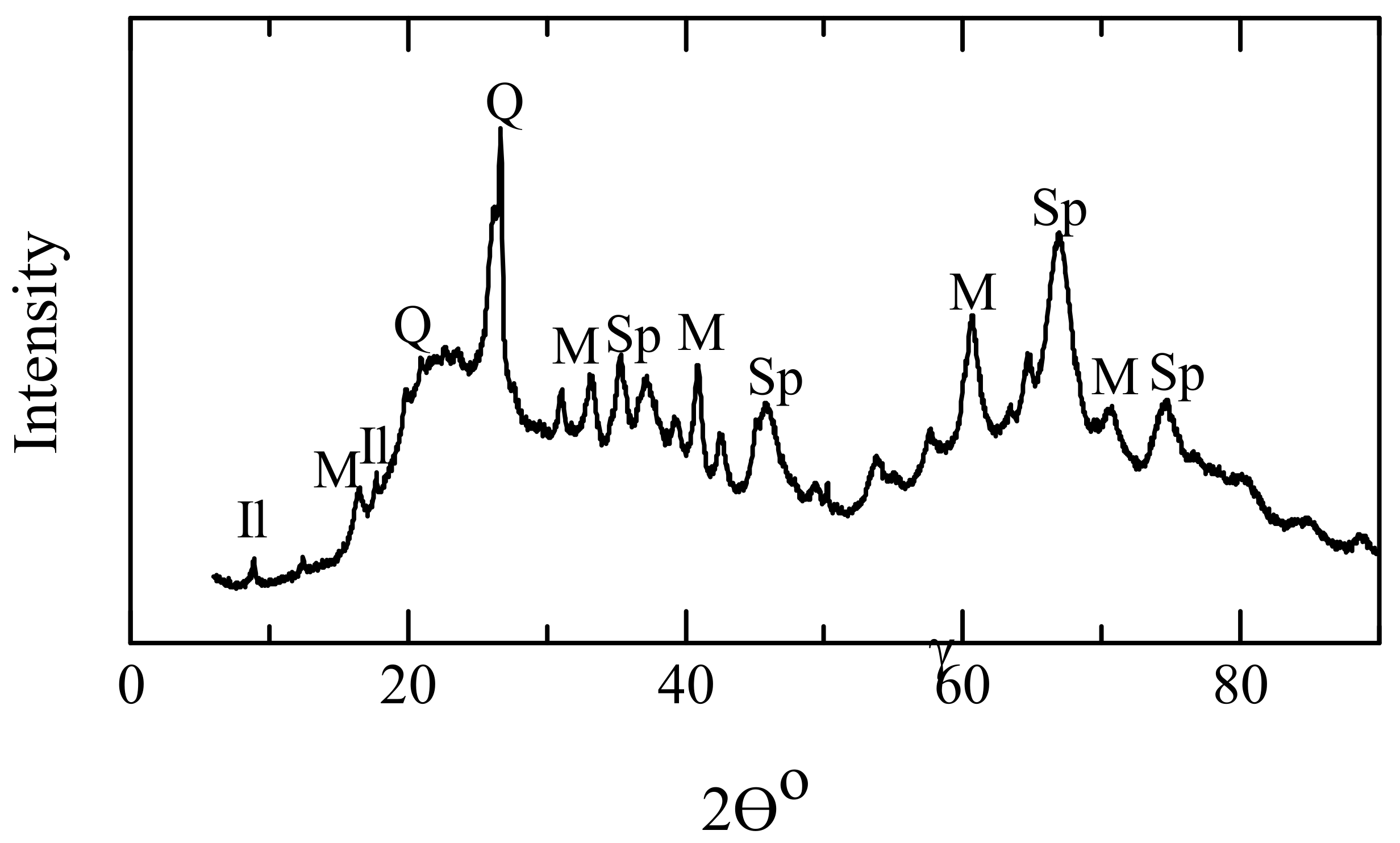
Figure 2.
Soluble Al2O3 content of the calcined kaolin samples from the two periods. The numbering of the samples refers to the collection chronology (error bars are smaller than plot symbols).
Figure 2.
Soluble Al2O3 content of the calcined kaolin samples from the two periods. The numbering of the samples refers to the collection chronology (error bars are smaller than plot symbols).

Figure 3.
Average infrared spectra of the calcined kaolin samples. The boxes highlight the spectral regions where the water features are located.
Figure 3.
Average infrared spectra of the calcined kaolin samples. The boxes highlight the spectral regions where the water features are located.
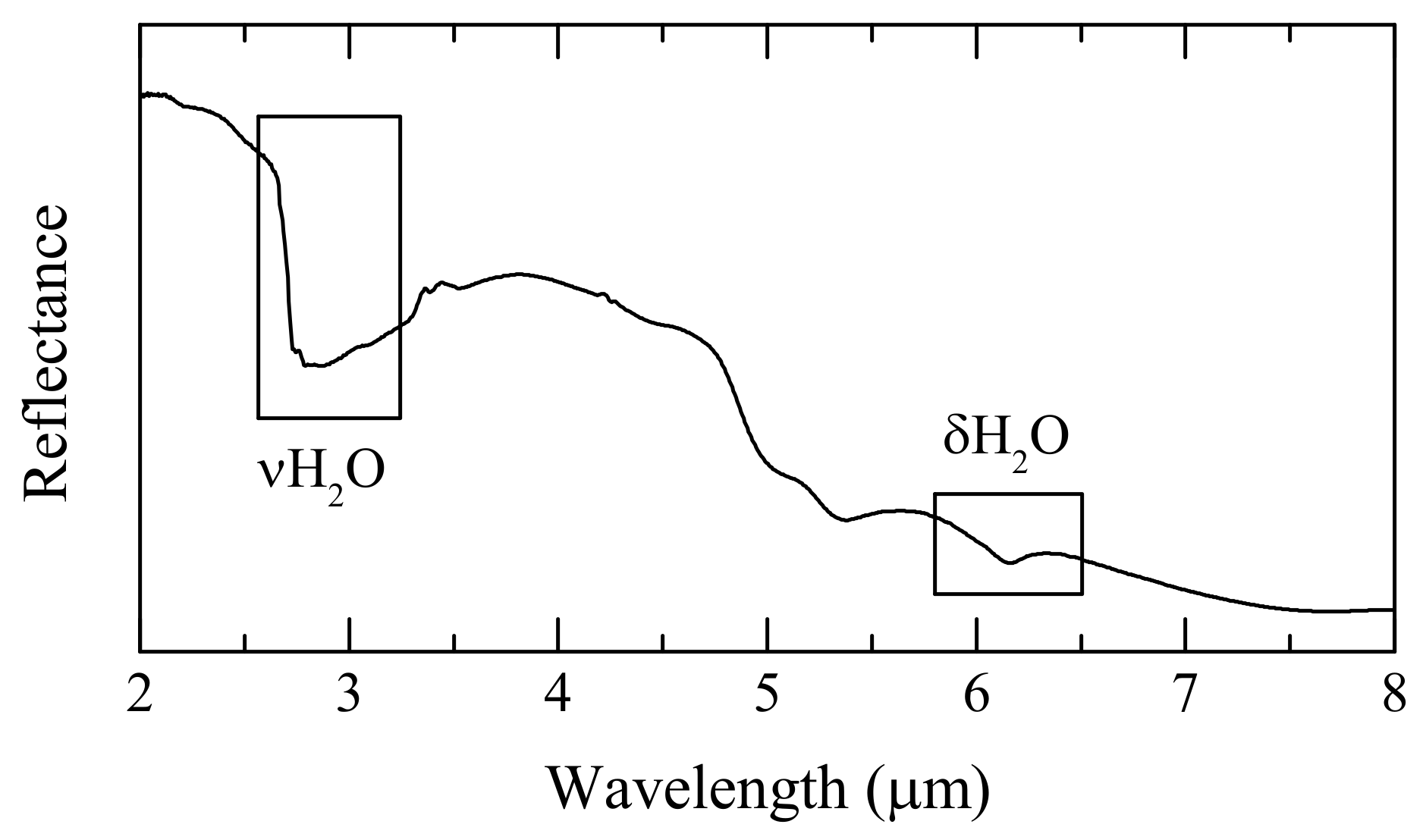
Figure 4.
(a) Raw; (b) standard normal variate (SNV); and (c) continuum removal (CR) processed infrared spectra of calcined kaolin in the 2.6 to 3.3 region. The markers indicate wavelength positions at 2.73, 2.75 and 2.78 .
Figure 4.
(a) Raw; (b) standard normal variate (SNV); and (c) continuum removal (CR) processed infrared spectra of calcined kaolin in the 2.6 to 3.3 region. The markers indicate wavelength positions at 2.73, 2.75 and 2.78 .
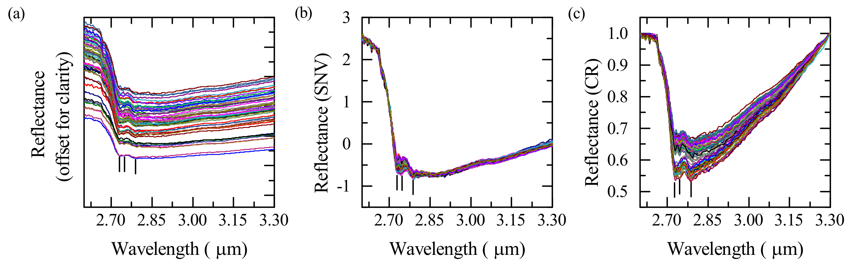
Figure 5.
(a) Raw; (b) SNV; and (c) CR processed infrared spectra of calcined kaolin in the 5.7 to 6.5 region. The markers indicate the center of the wavelength of the water feature at and the right shoulders in the SNV spectra at 6.24 and 6.27 .
Figure 5.
(a) Raw; (b) SNV; and (c) CR processed infrared spectra of calcined kaolin in the 5.7 to 6.5 region. The markers indicate the center of the wavelength of the water feature at and the right shoulders in the SNV spectra at 6.24 and 6.27 .

Figure 6.
Depth of the feature at compared with the soluble Al2O3 content, highlighting the differences between samples collected in the first and second periods.
Figure 6.
Depth of the feature at compared with the soluble Al2O3 content, highlighting the differences between samples collected in the first and second periods.
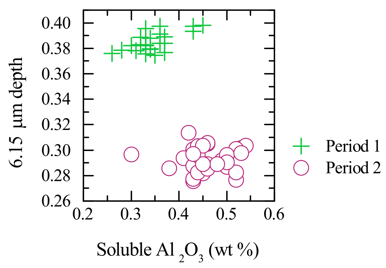
Figure 7.
(a) Measured vs. Predicted plot of the PLS-R model for the 5.7 to 6.5 range after SNV processing. LV = 3 in the calibration and validation samples. (b) Residuals plot of the PLS-R calibration.
Figure 7.
(a) Measured vs. Predicted plot of the PLS-R model for the 5.7 to 6.5 range after SNV processing. LV = 3 in the calibration and validation samples. (b) Residuals plot of the PLS-R calibration.
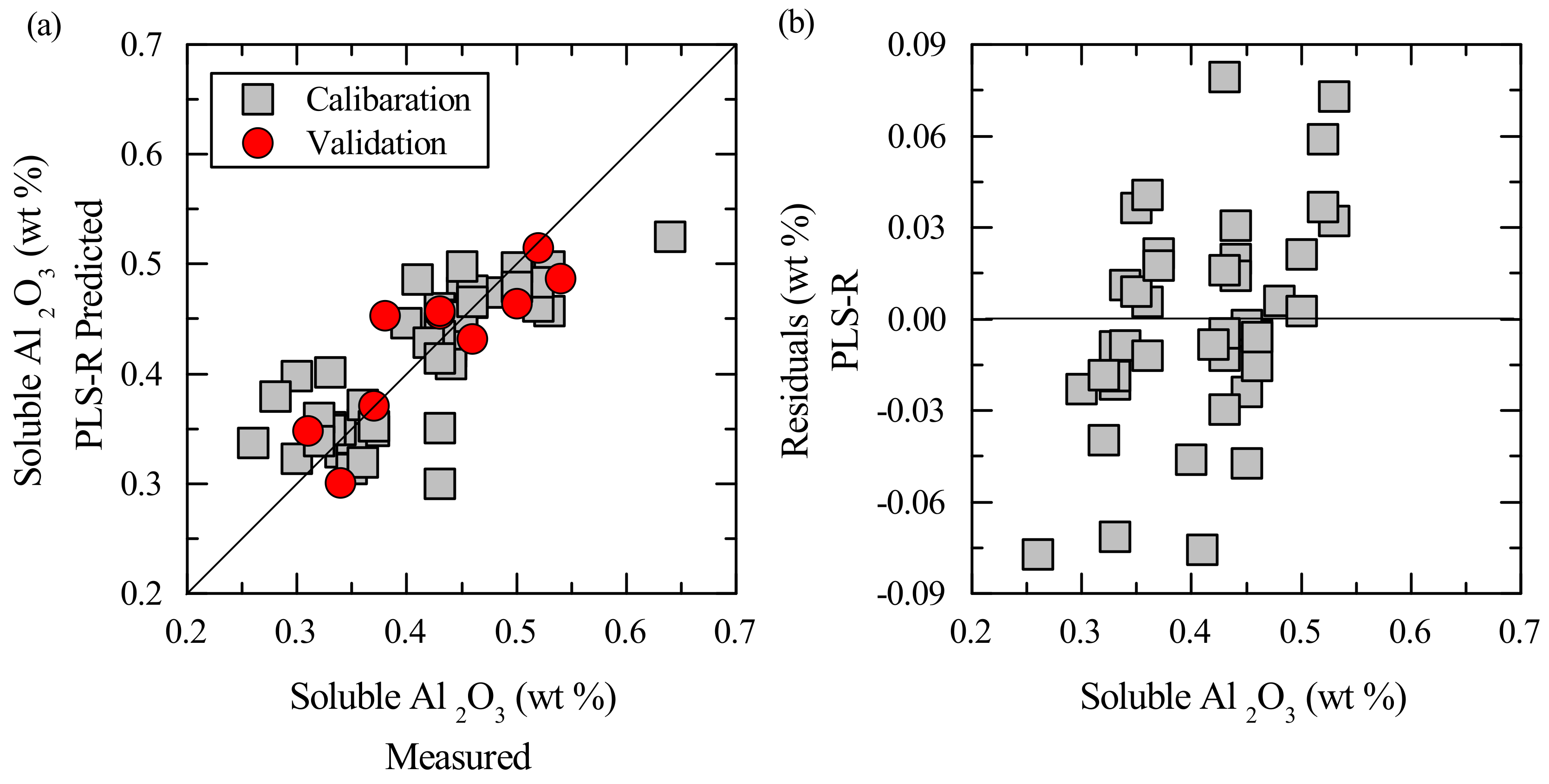
Figure 8.
(a) Measured vs. Predicted plot of the PLS-R model for the 5.7 to 6.5 range after SNV processing, including K2O, Fe2O3, and MgO as variables. LV = 2 in the calibration and validation samples. (b) Residuals plot of the PLS-R calibration.
Figure 8.
(a) Measured vs. Predicted plot of the PLS-R model for the 5.7 to 6.5 range after SNV processing, including K2O, Fe2O3, and MgO as variables. LV = 2 in the calibration and validation samples. (b) Residuals plot of the PLS-R calibration.
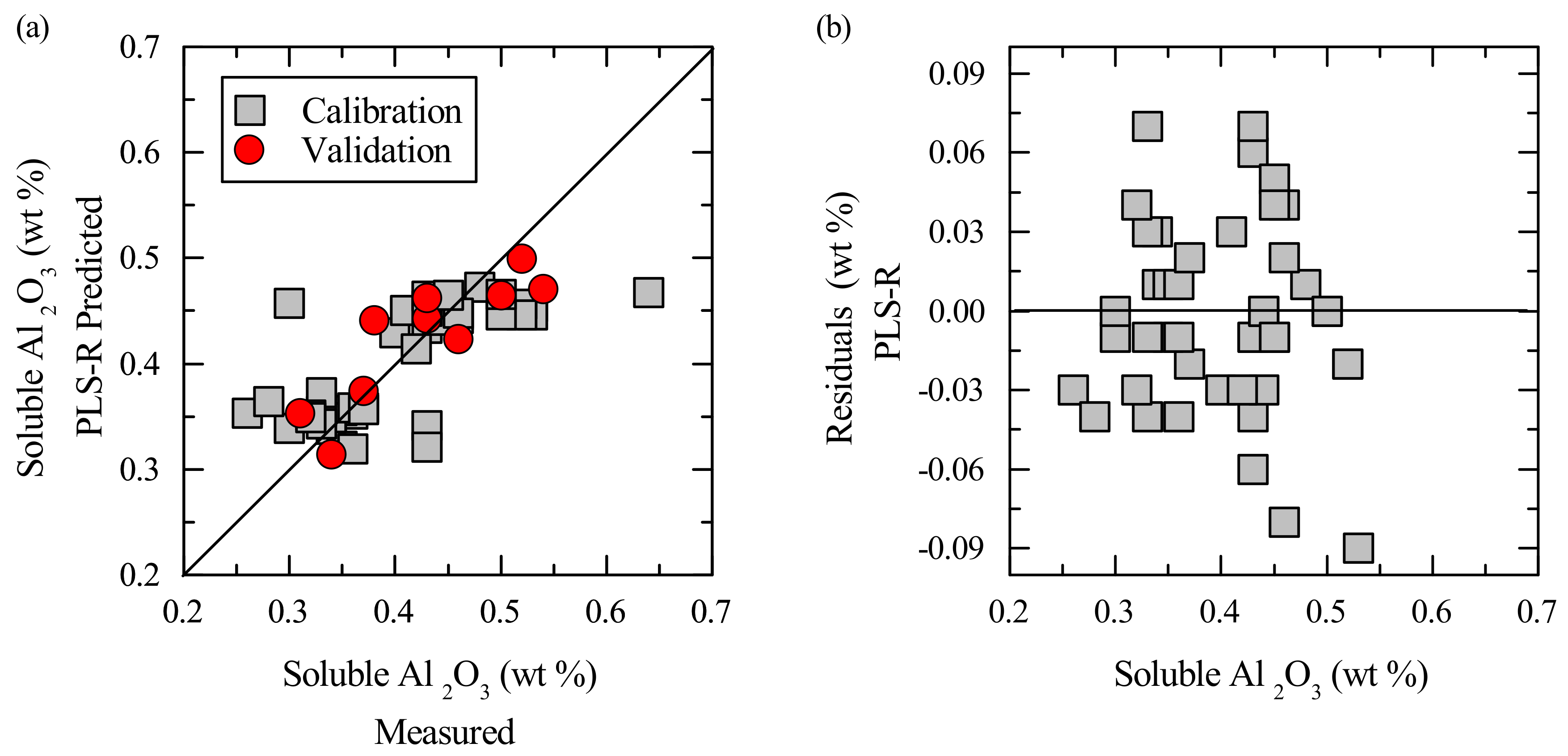
Figure 9.
(a) Measured vs. Predicted plot of the SVR model for the 5.7 to 6.5 range after CR processing. C = 3.1, = 0.46, SV = 19 in the calibration and validation samples. (b) Residuals plot of the SVR calibration.
Figure 9.
(a) Measured vs. Predicted plot of the SVR model for the 5.7 to 6.5 range after CR processing. C = 3.1, = 0.46, SV = 19 in the calibration and validation samples. (b) Residuals plot of the SVR calibration.

Table 1.
Chemical composition determined by X-ray fluorescence (XRF) and the soluble Al2O3 content of the calcined kaolin samples ().
Table 1.
Chemical composition determined by X-ray fluorescence (XRF) and the soluble Al2O3 content of the calcined kaolin samples ().
| Al2O3 | SiO2 | K2O | Fe2O3 | TiO2 | CaO | MgO | Na2O | LOI | Soluble Al | |
|---|---|---|---|---|---|---|---|---|---|---|
| Mean | 42.27 | 54.41 | 1.58 | 0.69 | 0.11 | 0.11 | 0.31 | 0.09 | 0.26 | 0.41 |
| Standard Deviation | 0.33 | 0.20 | 0.14 | 0.07 | 0.07 | 0.21 | 0.03 | 0.02 | 0.05 | 0.08 |
| Minimum | 41.07 | 53.85 | 1.25 | 0.58 | 0.04 | 0.04 | 0.26 | 0.05 | 0.17 | 0.26 |
| Median | 42.23 | 54.47 | 1.61 | 0.67 | 0.07 | 0.05 | 0.32 | 0.09 | 0.27 | 0.43 |
| Maximum | 42.91 | 54.69 | 1.80 | 0.78 | 0.32 | 1.31 | 0.35 | 0.13 | 0.37 | 0.64 |
Table 2.
Summary of the parameters and performance indicators of the best partial least squares regression (PLS-R) calibrations. LV: latent variable; RMSEC: root mean squared error of the calibration; RMSECV: root mean squared error of the cross-validation; RMSEP: root mean squared error of the prediction.
| Scenario | LV | RMSECV | RMSEC | RMSEP | ||
|---|---|---|---|---|---|---|
| Range | Processing | (wt %) | (wt %) | (wt %) | ||
| 2.6 to 3.3 | raw | 3 | 0.051 | 0.044 | 0.046 | 0.62 |
| SNV | 3 | 0.051 | 0.040 | 0.054 | 0.62 | |
| CR | 2 | 0.050 | 0.044 | 0.055 | 0.57 | |
| 5.7 to 6.5 | raw | 3 | 0.051 | 0.047 | 0.053 | 0.60 |
| SNV | 2 | 0.050 | 0.041 | 0.046 | 0.64 | |
| CR | 1 | 0.050 | 0.047 | 0.051 | 0.52 | |
Table 3.
Summary of the parameters and performance indicators of the best PLS-R calibrations, including K2O, Fe2O3, and MgO as variables.
Table 3.
Summary of the parameters and performance indicators of the best PLS-R calibrations, including K2O, Fe2O3, and MgO as variables.
| Scenario | LV | RMSECV | RMSEC | RMSEP | ||
|---|---|---|---|---|---|---|
| Range | Processing | (wt %) | (wt %) | (wt %) | ||
| 2.6 to 3.3 | raw | 3 | 0.053 | 0.034 | 0.046 | 0.62 |
| SNV | 4 | 0.053 | 0.036 | 0.061 | 0.62 | |
| CR | 3 | 0.050 | 0.036 | 0.056 | 0.57 | |
| 5.7 to 6.5 | raw | 3 | 0.053 | 0.036 | 0.052 | 0.57 |
| SNV | 2 | 0.050 | 0.036 | 0.039 | 0.53 | |
| CR | 1 | 0.050 | 0.036 | 0.043 | 0.54 | |
Table 4.
Summary of the optimisation parameters and performance indicators of the best support vector regression (SVR) calibrations.
Table 4.
Summary of the optimisation parameters and performance indicators of the best support vector regression (SVR) calibrations.
| Scenario | C | SV | RMSECV | RMSEC | RMSEP | |||
|---|---|---|---|---|---|---|---|---|
| Range | Processing | (wt %) | (wt %) | (wt %) | ||||
| 2.6 to 3.3 | raw | 15.0 | 0.80 | 20 | 0.055 | 0.048 | 0.050 | 0.57 |
| SNV | 3.5 | 0.40 | 21 | 0.052 | 0.023 | 0.050 | 0.86 | |
| CR | 3.5 | 0.50 | 22 | 0.048 | 0.031 | 0.048 | 0.71 | |
| 5.7 to 6.5 | raw | 5.0 | 0.31 | 30 | 0.056 | 0.045 | 0.047 | 0.59 |
| SNV | 4.0 | 0.53 | 17 | 0.048 | 0.027 | 0.047 | 0.80 | |
| CR | 3.1 | 0.46 | 19 | 0.046 | 0.025 | 0.044 | 0.87 | |
© 2018 by the authors. Licensee MDPI, Basel, Switzerland. This article is an open access article distributed under the terms and conditions of the Creative Commons Attribution (CC BY) license (http://creativecommons.org/licenses/by/4.0/).
Share and Cite
MDPI and ACS Style
Guatame-Garcia, A.; Buxton, M. Prediction of Soluble Al2O3 in Calcined Kaolin Using Infrared Spectroscopy and Multivariate Calibration. Minerals 2018, 8, 136. https://doi.org/10.3390/min8040136
AMA Style
Guatame-Garcia A, Buxton M. Prediction of Soluble Al2O3 in Calcined Kaolin Using Infrared Spectroscopy and Multivariate Calibration. Minerals. 2018; 8(4):136. https://doi.org/10.3390/min8040136
Chicago/Turabian StyleGuatame-Garcia, Adriana, and Mike Buxton. 2018. "Prediction of Soluble Al2O3 in Calcined Kaolin Using Infrared Spectroscopy and Multivariate Calibration" Minerals 8, no. 4: 136. https://doi.org/10.3390/min8040136
Note that from the first issue of 2016, this journal uses article numbers instead of page numbers. See further details here.