Multibody Dynamic Stress Simulation of Rigid-Flexible Shovel Crawler Shoes

Abstract

Electric shovels are used in surface mining operations to achieve economic production capacities. The capital investments and operating costs associated with the shovels deployed in the Athabasca oil sands formation are high due to the abrasive conditions. The shovel crawler shoes interact with sharp and abrasive sand particles, and, thus, are subjected to high transient dynamic stresses. These high stresses cause wear and tear leading to crack initiation, propagation and premature fatigue failure. The objective of this paper is to develop a model to characterize the crawler stresses and deformation for the P&H 4100C BOSS during propel and loading using rigid-flexible multi-body dynamic theory. A 3-D virtual prototype model of the rigid-flexible crawler track assembly and its interactions with oil sand formation is simulated to capture the model dynamics within multibody dynamics software MSC ADAMS. The modal and stress shapes and modal loads due to machine weight for each flexible crawler shoes are generated from finite element analysis (FEA). The modal coordinates from the simulation are combined with mode and stress shapes using modal superposition method to calculate real-time stresses and deformation of flexible crawler shoes. The results show a maximum von Mises stress value of 170 MPa occurring in the driving crawler shoe during the propel motion. This study provides a foundation for the subsequent fatigue life analysis of crawler shoes for extending crawler service life.

1. Introduction

The electric shovel is widely used in the surface mining operations. The lower works of the shovel consist of propel and crawler systems, as shown in Figure 1. The crawler dimensions, material properties and shovel load acting on the lower works in Figure 1 are based on the P&H 4100C BOSS electric shovel [1,2]. The crawler consists of a crawler track assembly, front and rear idlers, lower rollers and guide rails [3]. The crawlers are made up of shoes that are connected together by link pins to form a continuous chain. The shovel reliability depends on crawler track service life. The crawler supports the entire machine load and payload during its operating cycle. The dynamic loads from this interaction can cause stress loading of crawlers, wear and tear, crack and eventual failure. Frimpong and Li [4] modeled the interaction between the shovel dipper and oil sands formation and determined the dynamic stresses in the boom during crowding and digging using rigid-flexible multi-body dynamics theory. The results showed that the von Mises stress at the joint location between the boom and upper structure exceeded the material yield strength. Frimpong and Li [5] extended their study [4] to analyze stresses in the shovel front-end components. They found the highest stresses around the region where the hoist rope is attached to the dipper.

Frimpong and Thiruvengadam [6,7,8] studied the rigid multi-body dynamic simulation of shovel crawler-terrain interactions during propel of the P&H 4100C BOSS shovel. They developed a 3-D virtual model of crawler-terrain interactions in MSC ADAMS. Their results included shoe kinematics, contact forces on shoes, joint forces in the link pin and total terrain deformation. The stress distributions are required to study fatigue life for extended service. Thus, the objective of this study is to model the stress loading of the crawler shoes during the shovel’s operating cycle within MSC ADAMS View/Flex/Durability and MSC NASTRAN [9,10,11,12,13] as a basis for future fatigue failure life studies.

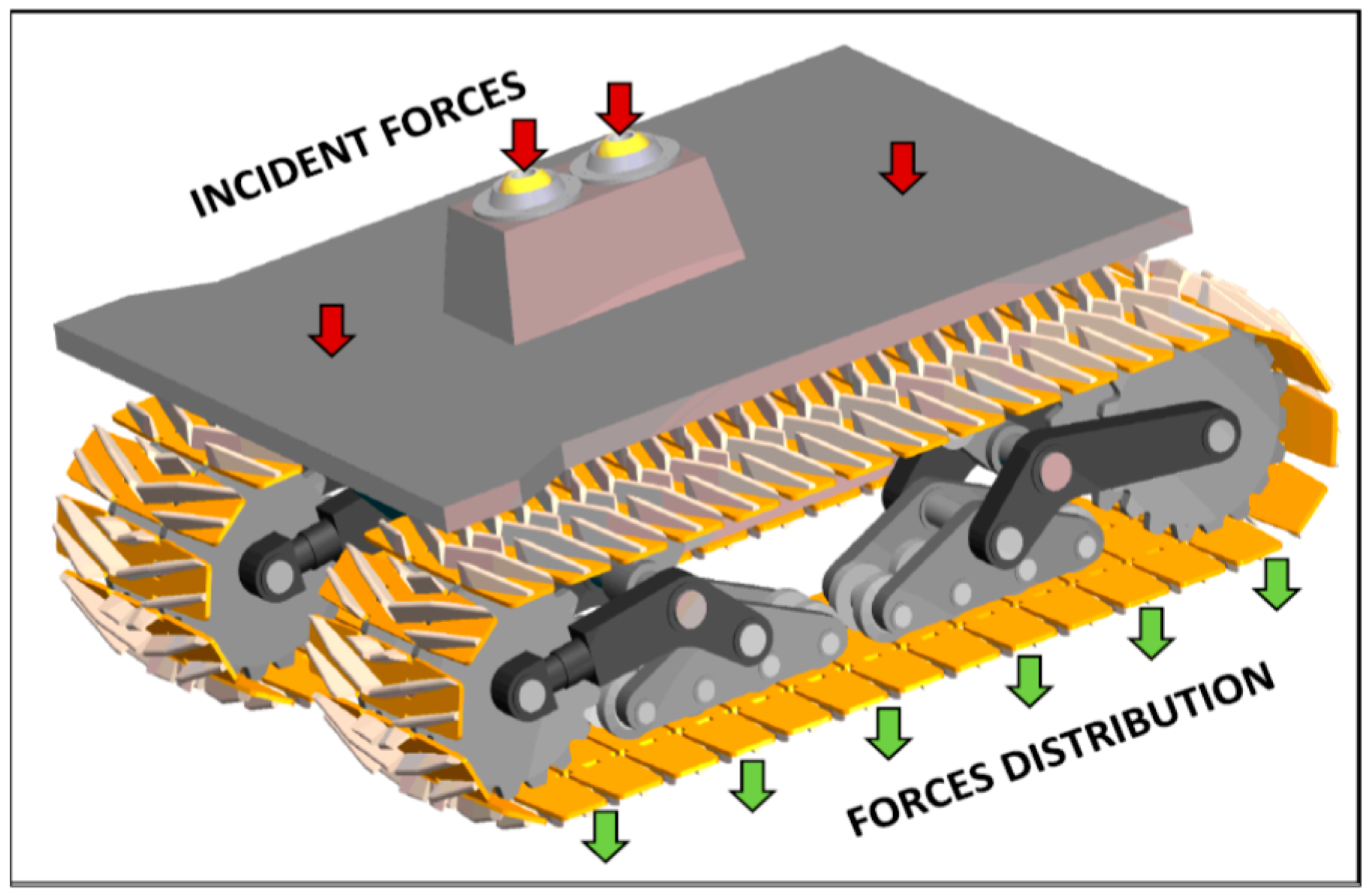
2. Rigid-Flexible Multi-Body Dynamics of Crawler-Terrain Interactions

Frimpong and Thiruvengadam [6,7,8] developed the crawler-terrain assembly (Figure 1) based on P&H 4100C Boss shovel crawler dimensions (

Table 1. Crawler dimensions of P&H 4100C electric shovel [1].

Measurements	Dimensions
Width of Crawler Shoes	3.505 m
Width of Crawler	12.8 m
Length of Crawlers	11.6 m

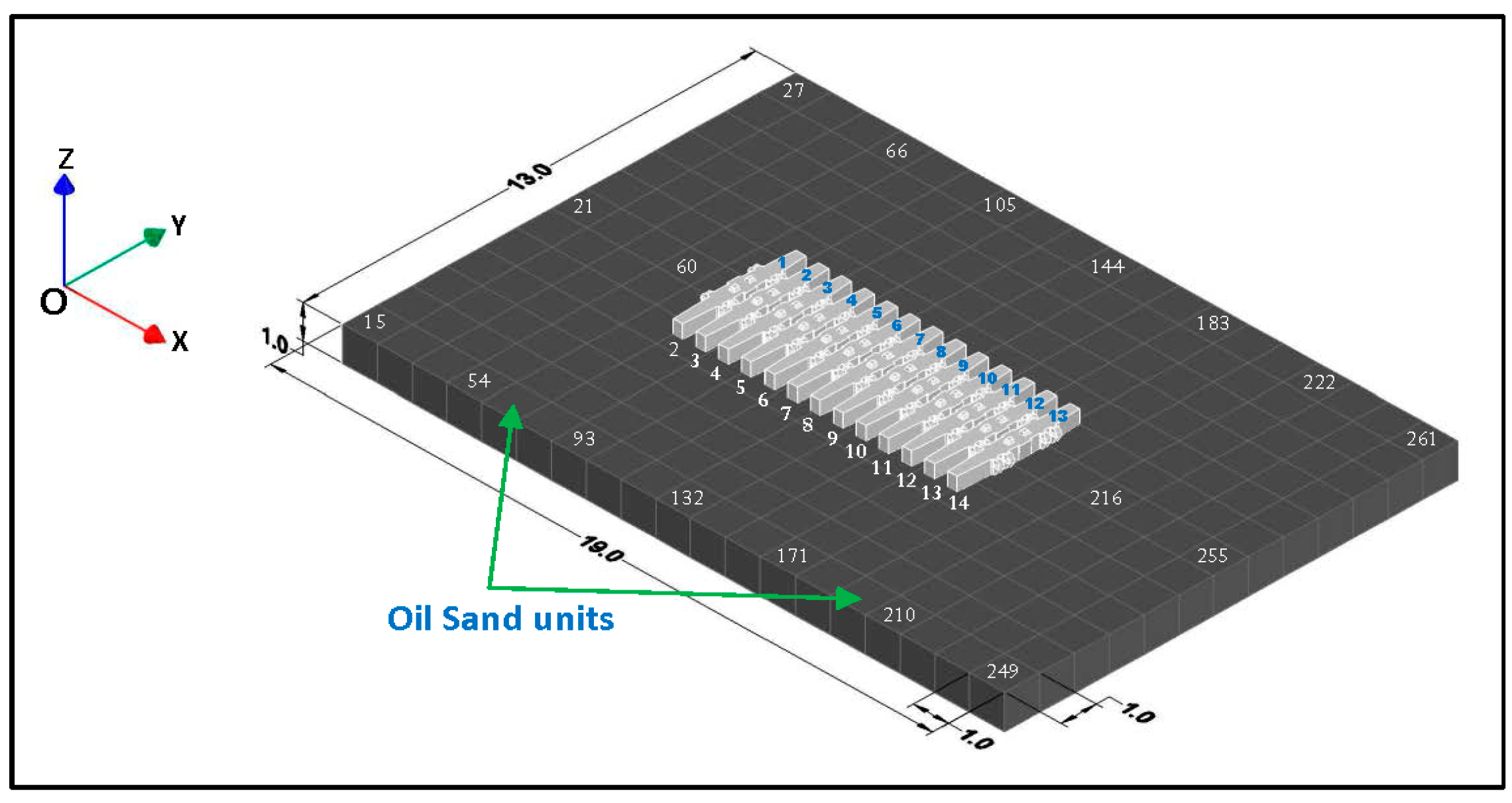
). The crawler shoes were generated in Solidworks, based on the actual crawler shoe for the same shovel [1,2]. The oil sand terrain is modeled as a continuous system with a finite number of 2-degree of freedom (DOF) spring damper oil sand units. The oil sand terrain had a total length, width and depth of 70, 32.5 and 2 m, respectively. Each oil sand unit size was 7 m × 7 m × 2 m, resulting in 50 oil sand units.

This study makes two changes to the oil sand model, (i) terrain size reduction to 19 m × 13 m × 1 m (from 70 m × 32.5 m × 2 m) and (ii) unit size reduction to 1 m × 1 m × 1 m (from 7 m × 7 m × 2 m), resulting in 247 oil sand units. The decrease in oil sand unit size increases the total number of parts in the multi-body system, but can accurately approximate the oil sands load deformation model. Any further decrease in the oil sand unit size caused increased computational time and, hence, was not attempted. Figure 2 shows the geometric track model, comprising 13 shoes, in contact with the terrain. The terrain shows the footprint of a single crawler track with 4 to 5 m of extended space around the track. Any additional extended space had a negligible effect on the total deformation of the terrain and crawler-terrain interaction dynamics.

Table 2. Material properties of the system

Body	Density (kg/m3)	Mass (kg)	Elastic Modulus	Poisson’s Ratio	Stiffness (k) MN/m	Damping (c) (kNs/m)
Crawler Shoe	7847.25	4489.63	200 GPa	0.3	-	-
Oil-sand	1600.0	1600	20 MPa	0.3	20	120

contains stiffness (k) and damping (c) characteristics and terrain and crawler properties. The shoes and oil sand units are identified by numbers 2 to 261, with Part 1 being the default ground link in MSC ADAMS, as shown in Figure 2.

The 13 crawler shoes are numbered 1 to 13 in blue (Figure 2) as alternate names for Parts 2 to 14, with part 7 as shoe #6. The reference global coordinate system is located at point O, as shown in Figure 2. A rigid virtual prototype simulator is developed in MSC ADAMS and modified to generate the rigid–flexible prototype model.

The kinematics and applied forces used to generate the rigid prototype simulator are discussed in the following paragraphs of this section.

Kinematic Constraints: These include joint, spring-damper element, and motion constraints. The rigid crawler shoes are connected to each other using spherical and parallel primitive joint constraints. Oil sand units are held together with spherical and in-plane primitive joints. Each unit is connected to the ground link using a spring-damper element with a 1-m length. The cross-sectional area of the unit is 1 m² with a spring length of 1 m. The stiffness (k) is equal to the elastic modulus of the oil sand (E) in Table 2. The translation propel motion of the crawler is obtained by imposing a motion constraint (in Equation (1)) on shoe 13 at its center of mass (COM) in the global positive x-direction using the cubic STEP function in MSC ADAMS.

$$v_x\left(t\right)=\left[\begin{array}{ll}\underset{¯}{\mathrm{Propelling}}& \\ 0.012t^2-0.0016t^3& ;0\le t\le 5s\\ 0.1& ;5<t\le 10s\\ 0.1+\left\{\left(-0.1\right)\frac{{\left(t-10\right)}^2}{25}\left(3-2\frac{\left(t-10\right)}{5}\right)\right\}& ;10<t\le 15s\\ \underset{¯}{\mathrm{Loading}}& \\ Disabled& ;15<t\le 40s\end{array}\right]m/s$$

(1)

The crawler track moves in the remaining five DOFs (two translations and three rotations) during propel. This motion constraint is deactivated when loading begins to allow six-DOF movements. The motion constraint in Equation (1) causes the crawler track to (i) accelerate from rest; (ii) propel at constant velocity; and (iii) decelerate to rest at the working face. Motion constraints are also imposed on oil sand units at their COMs to allow 2 DOFs. Frimpong and Thiruvengadam [6] define the kinematic equations governing the joint and motion constraints between adjacent crawler shoes and oil sand units.

External Forces on Crawler Shoes: External forces on crawler shoes are (i) contact forces between crawler shoes and terrain; (ii) gravity; and (iii) distributed loads on crawler tracks. The gravity force is a user-defined input in MSC ADAMS. The contact force is a time varying force comprising normal and frictional forces and frictional torque. This force is estimated using in-built contact algorithms in MSC ADAMS and the parameters in

Table 3. Contact parameters used in the study [8,10,14].

Normal Force		Friction Force
Contact Stiffness (k, N/m)	1.0 × 108	Static Coefficient (µs)	0.4
Max. Contact Damping (cmax, N·s/m)	1.0 × 104	Dynamic Coefficient (µd)	0.3
Force Exponent (e)	2.0	Static transition velocity (Vst, m/s)	0.01
Max. Penetration Depth (d, m)	1.0 × 10−4	Dynamic transition velocity (Vd, m/s)	0.1

[8].

The total load comprises shovel weight (minus crawler weight) and dipper payload. The shovel weight is constant but the dipper payload varies with time and fill factor. 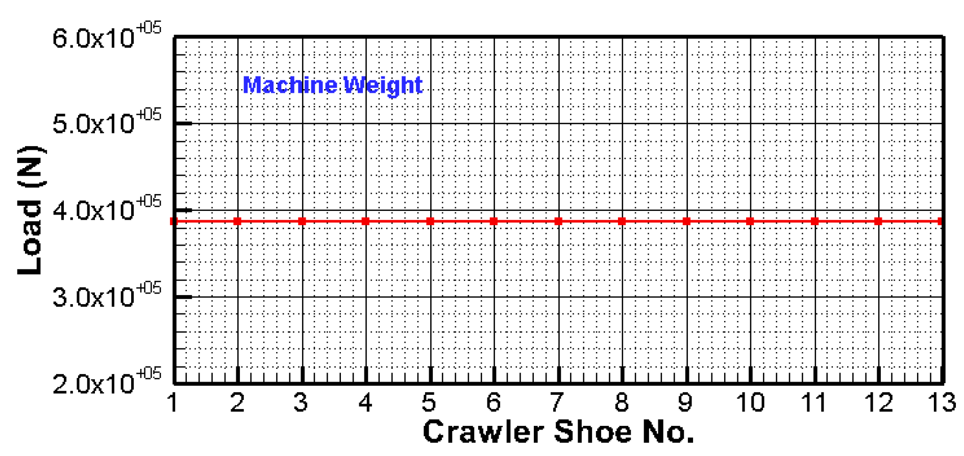The shovel cycle consists of (i) propel to the working face (0 < t < 15 s); (ii) material excavation (15 < t < 22.5 s); (iii) hoisting and swinging from the face to haul truck (22.5 < t < 30 s); (iv) material dumping into haul truck (30 < t < 33.5 s); and (v) swinging after dumping to the digging face (33.5 < t < 40 s). During propel, the load on each crawler shoe is only due to the empty machine weight. The total machine weight for the P&H 4100C BOSS is 1,410,184 kg [1]. The total machine load (excluding crawler shoe weight) for the P&H 4100C BOSS is 630,185 kg. This load is distributed uniformly on crawler shoes 1–13 in Figure 3. Therefore, the machine load/shoe in contact with the ground is equal to 386.4 kN.

During digging, non-uniform machine and dipper loads act on the crawler shoes. The total dipper weight for the P&H 4100 C BOSS is 890 kN. It is assumed that (i) dipper load is uniformly distributed on the crawler tracks, and thus, dipper load/track is 445 kN; (ii) dipper load acts only on the 7 front crawler shoes; and (iii) shoes 1, 2, 3, 4, 5 and 6 do not support any dipper load and, therefore, the highest dipper load acts on shoe 13 and the lowest on shoe 7. 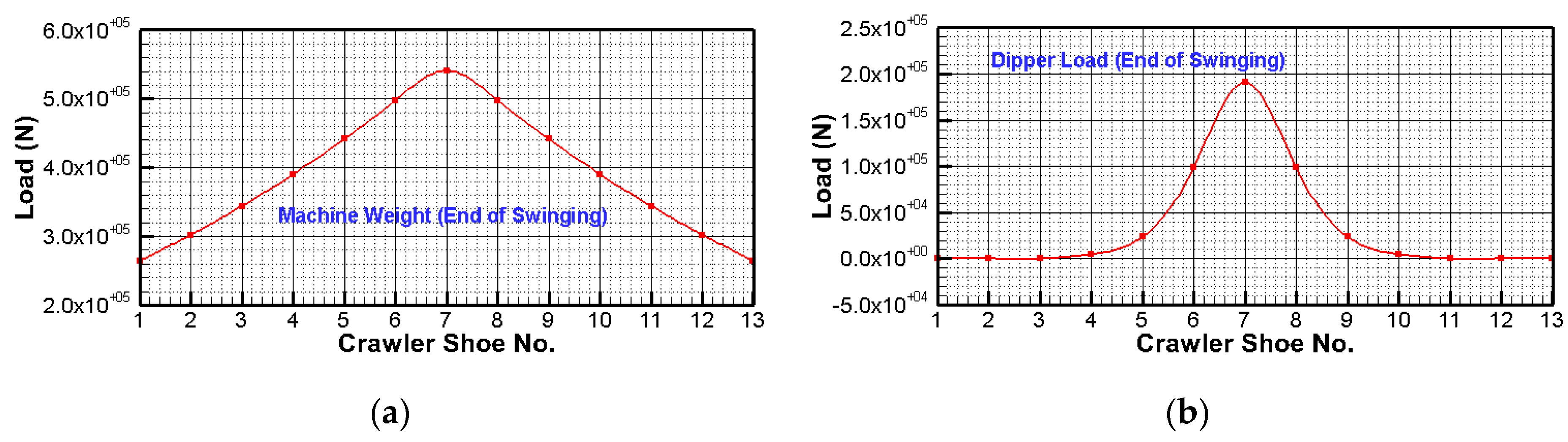The total distributed load on each crawler shoe is equal to machine plus dipper load, as shown in Figure 4. During swinging, the maximum machine and dipper loads shift to the middle shoes, resulting in symmetric load distribution, with the highest load on shoe 7, at the end of swinging, as shown in Figure 5. During dumping, the dipper load reduces to zero and at the end of dumping, only the symmetric machine load, in Figure 5a, acts on crawler shoes 1–13. During return, the machine load is redistributed and, at the end of return, the uniform load in Figure 3 acts on shoes 1–13.

The cubic STEP function defines the total load as a function of load and time. For example, crawler shoe 7 has a total load of (i) 386.4 kN for propel (M); (ii) 384 kN at the end of digging (D); (iii) 732 kN at the end of swinging (S); (iv) 541 kN at the end of dumping (G); and (v) 386.4 kN at the end of return (M). Equation (2) defines the step function for crawler shoe 7.

$$\mathrm{Load}=\left[\begin{array}{ll}M& \forall t\le 15s\\ M+(D-M){\left(\frac{t-15}{7.5}\right)}^2\left[3-2\left(\frac{t-15}{7.5}\right)\right]& \forall 15<t<22.5s\\ D& \forall t=22.5s\\ D+(S-D){\left(\frac{t-22.5}{7.5}\right)}^2\left[3-2\left(\frac{t-22.5}{7.5}\right)\right]& \forall 22.5<t<30s\\ S& \forall t=30s\\ S+(G-S){\left(\frac{t-30}{3.5}\right)}^2\left[3-2\left(\frac{t-30}{3.5}\right)\right]& \forall 30<t<33.5s\\ G& \forall t=33.5s\\ G+(M-G){\left(\frac{t-33.5}{6.5}\right)}^2\left[3-2\left(\frac{t-33.5}{6.5}\right)\right]& \forall 33.5<t<40s\\ M& \forall t=40s\end{array}\right]N$$

(2)

Similar load distribution equations can be obtained for other crawler shoes, as shown in Figure 6. Figure 6 shows that the load at the end of digging and swinging operations on each crawler shoe is equal to the sum of the machine weight and dipper payload (in Figure 4 and Figure 5). These loads are applied as point loads at the centroid of each crawler shoe. Figure 7 shows the virtual rigid body crawler-terrain simulator. The rigid crawler shoes are replaced with flexible crawler shoes to simulate the rigid–flexible crawler-terrain interactions.

3. Rigid–Flexible Multi-Body Model

The front and middle sets of crawler shoes are subjected to maximum loads from both machine and dipper payloads. These maximum loads can cause a large stress buildup in the crawler shoes that can cause fatigue failure. This study captures the stresses on the front and middle crawler shoes using rigid–flexible multibody dynamics theory.

The three front crawler shoes (11, 12 and 13) and the middle ones (6, 7 and 8) are made flexible using modal neutral file (MNF) [11,12,15]. An MNF file is generated for each shoe using MSC NASTRAN [13]. The front shoes capture the digging loads and the middle shoes capture the swinging loads.

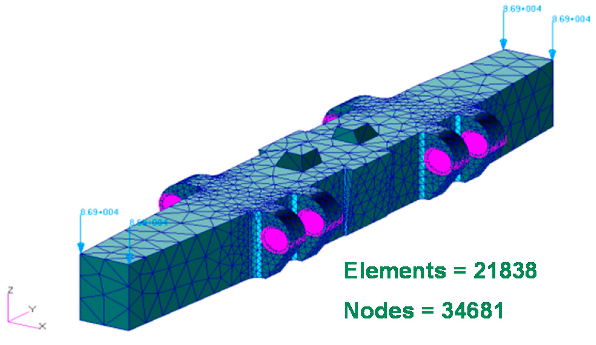
Generation of Modal Neutral File (MNF): The geometric models of shoes 6, 7, 8, 11, 12 and 13 are imported into MSC PATRAN to generate a finite element (FE) mesh using 10-node tetrahedral elements. The shoe material is assumed to be linear and isotropic. Table 2 contains the material properties for generating the flexible body. The machine load on each crawler shoe is scaled to generate the time varying loads during shovel operation. Four attachment nodes with 6 DOFs are generated at the joint locations in the crawler track assembly. Rigid body spider web elements (RBE2) are used to connect the attachment nodes at the joint center to the surface nodes around the hole of the joint [15].

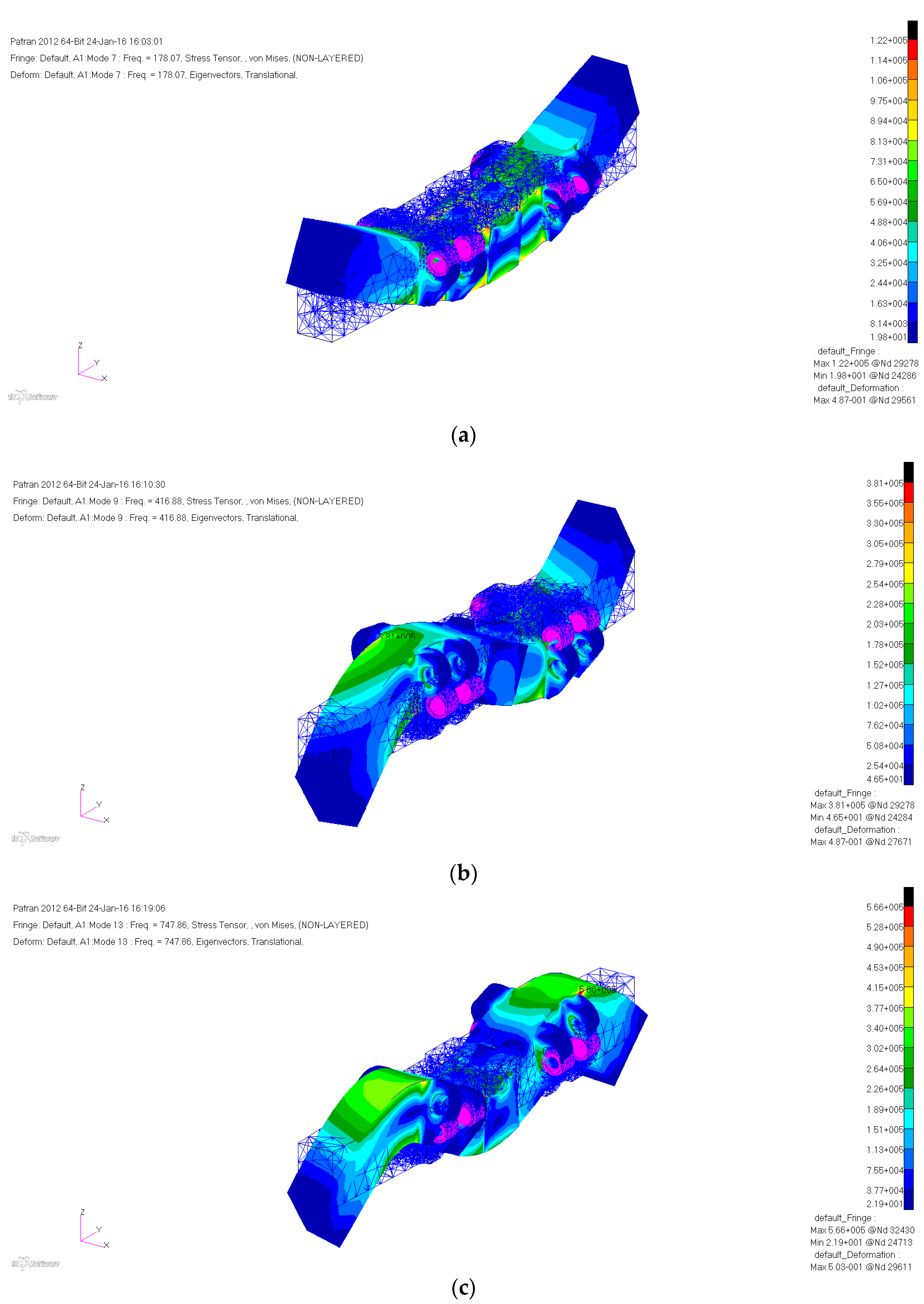
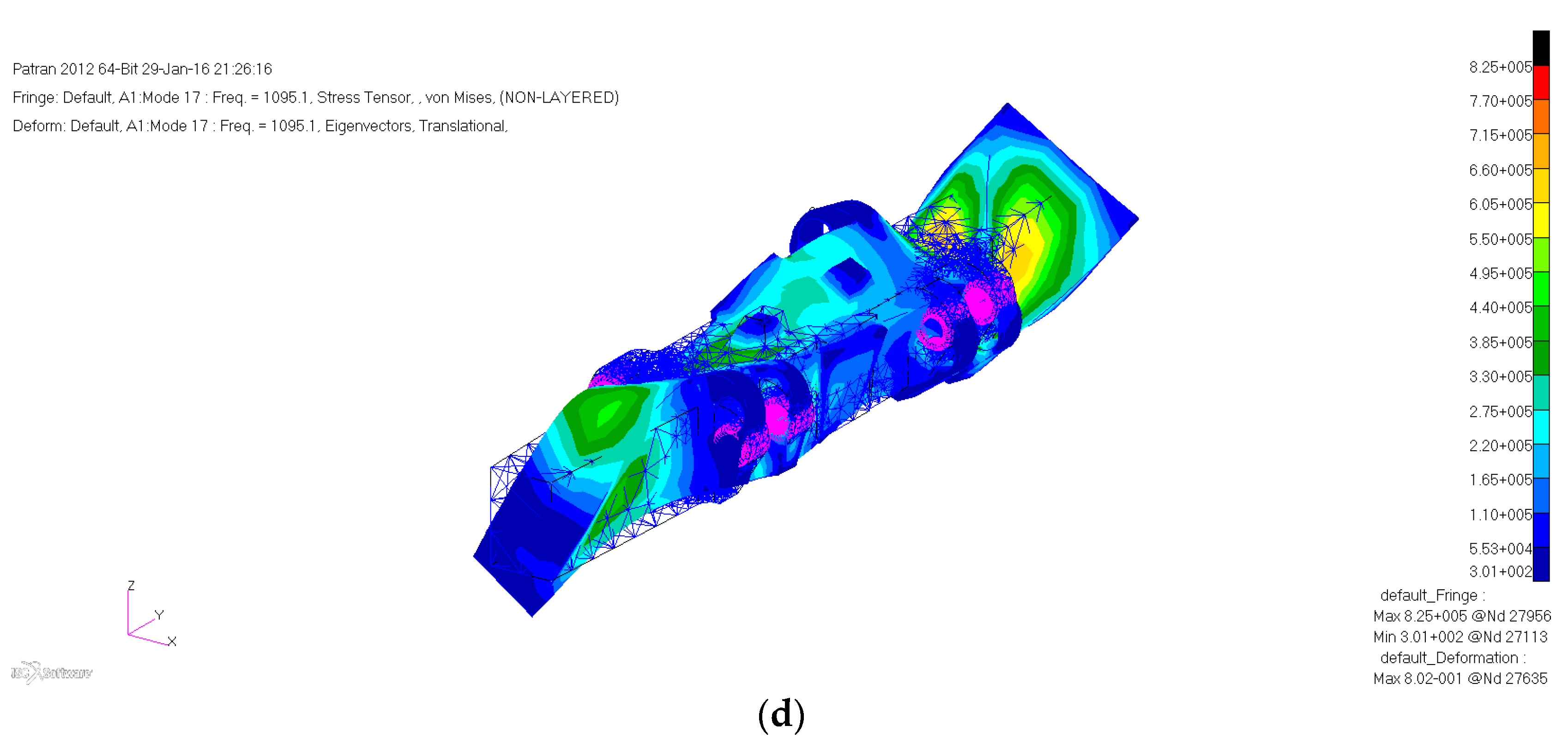
The component mode synthesis (CMS) from Frimpong and Li [4], and Craig [16], is carried out on the meshed crawler shoes using the modal analysis solver in MSC NASTRAN. CMS consists of constraint and fixed boundary normal modes. Seventy six fixed boundary mode shapes are exported from MSC NASTRAN into MNF. CMS generates 100 component modes that include 24 constraint and 76 fixed boundary modes. These modes are ortho-normalized with associated natural frequencies. The first six orthogonalized Craig-Bampton modal basis are rigid-body modes with natural frequencies. These are deactivated during multi-body dynamic simulation in MSC ADAMS. A sample mesh for shoe 7 and the different mode shapes with frequencies (f) up to 1200 Hz are shown in Figure 8 and Figure 9. The reduced modal results are exported into an MNF file, which contains generalized stiffness and mass matrices, Eigenvalues, mode shapes, stress modes, modal loads, nodal coordinates, attachment nodes and inertia invariants [11].

The MNFs are imported into MSC ADAMS rigid virtual prototype model, in Figure 7, to create flexible shoes. After creating the flexible shoes, changes are made to their joint connections, contact forces, distributed loads and modal damping to develop the rigid–flexible virtual prototype simulator for the crawler-terrain interactions.

Joint constraints: The spherical and parallel primitive joints are replaced with two revolute joints between rigid–flexible and flexible–flexible crawler shoes.

Contact Force: The rigid–flexible multi-body system uses a flexible–rigid solid contact model to capture the contact between each flexible crawler shoe and rigid oil sand mass unit. Table 3 contains the parameters for the contact forces.

Modal loads: The MNF file contains modal loads for the uniformly distributed machine weight for flexible FEA crawler shoes 6, 7, 8 11, 12 and 13, as shown in Figure 8. These loads are applied using the MFORCE element in MSC ADAMS. The modal loads are scaled as a function of time using the cubic STEP Function in MSC ADAMS, in Figure 6, for shovel propel and loading.

Modal Damping: From the modal analysis, 100 ortho-normalized component modes, including 6 rigid-body modes with associated frequencies, are generated for the MNF file. Modal damping ratios are specified for all flexible crawler shoes in the MNF file [11]. The critical damping ratios (ζ_i) for mode i = 7, 8…N, as a function of modal frequency (f_i), for flexible crawler shoes 6, 7, 8 11, 12, and 13, shown in Equation (3), are applied using FXFREQ function in MSC ADAMS [11,15]. 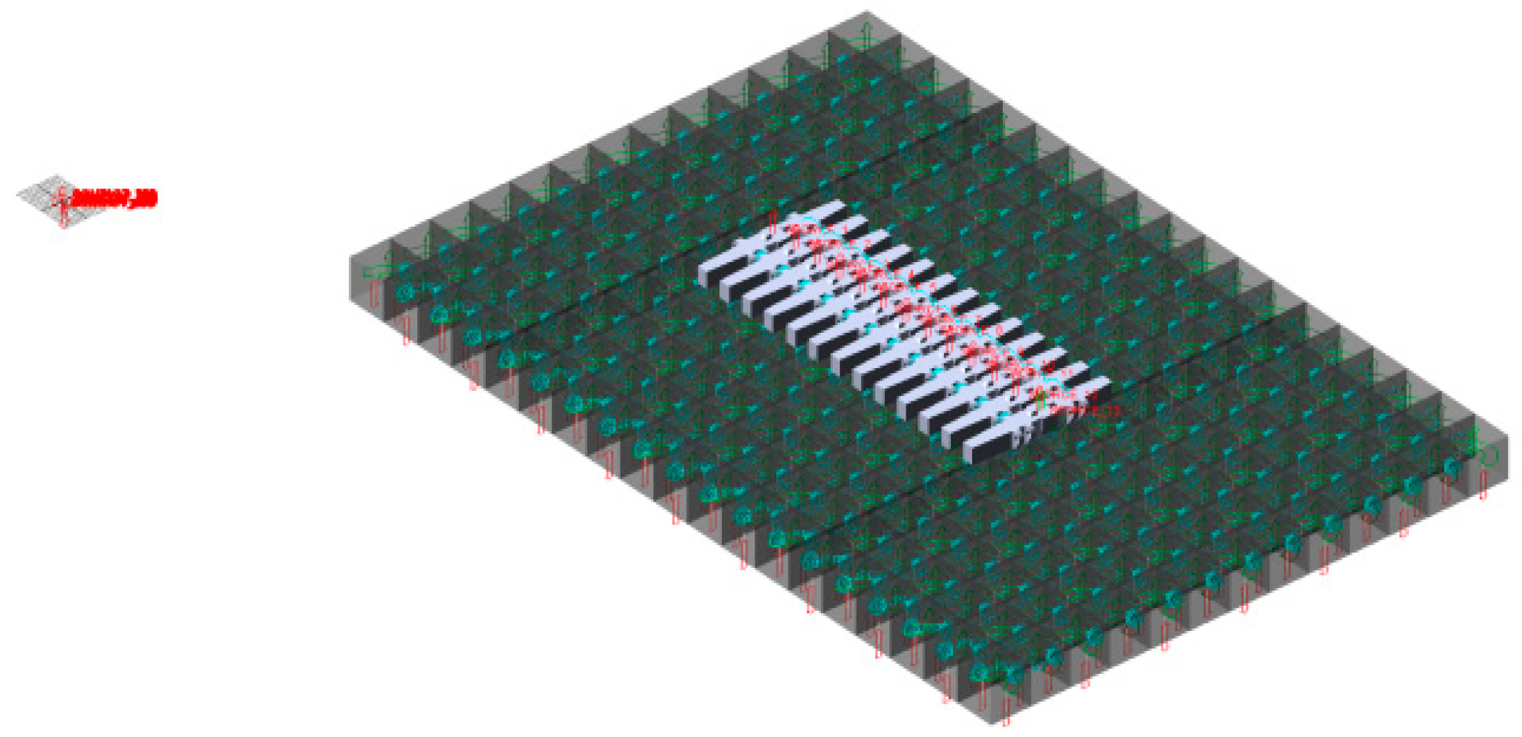N (=100) is the number of modes. The completed 3-D virtual model for simulating the rigid–flexible crawler-terrain interaction is shown in Figure 10.

$${\mathsf{\zeta }}_i=\left[\begin{array}{l}0.005;f_i\le 1000Hz\\ 0.005+(1-0.005){\left(\frac{f_i-1000}{9000}\right)}^2\left[3-2\left(\frac{f_i-1000}{9000}\right)\right];1000<f_i<10000Hz\\ 1;f_i>10000Hz\end{array}\right]i=7,8,\dots N$$

(3)

The differential-algebraic equations (DAE) governing the simulation of the rigid–flexible crawler-formation interaction is derived from the Lagrange’s equation [11] as Equation (4).

$$\begin{array}{l}M\ddot{\mathsf{\xi }}+\dot{M}\dot{\mathsf{\xi }}-\frac{1}{2}{\left[\frac{\partial M}{\partial \mathsf{\xi }}\dot{\xi }\right]}^T\dot{\xi }+K\mathsf{\xi }+f_g+D\dot{\xi }+{\left[\frac{\partial \Psi }{\partial \mathsf{\xi }}\right]}^T\mathsf{\lambda }=Q\\ \Psi =0\end{array}$$

(4)

$M$ is the generalized mass matrix, $\mathsf{\xi }$ is the generalized coordinates vector, $K$ is the generalized stiffness matrix, $f_g$ is the generalized gravitational force, $D$ is the modal damping matrix, $\mathsf{\Psi }$ is the vector of algebraic constraint equations, $\mathsf{\lambda }$ is the Lagrange multipliers, and $Q$ is the generalized applied forces. The generalized coordinates of the rigid–flexible body, $\mathsf{\xi }$, are given by Equation (5).

$$\mathsf{\xi }=\left[\begin{array}{l}x\\ \mathsf{\gamma }\\ q\end{array}\right]$$

(5)

$x={\left[xyz\right]}^T$ is the global position vector for the rigid/flexible body coordinate system origin; $\mathsf{\gamma }={\left[\mathsf{\psi }\mathsf{\theta }\mathsf{\phi }\right]}^T$ is the fixed body 3-1-3 Euler angles that relate the orientation of the rigid/flexible body to the global coordinate system; and $q={\left[q_7{q}_8\dots q_N\right]}^T$ is the flexible body modal coordinates vector. Equation (4) is integrated over time using the GSTIFF integrator with SI2 formulation in MSC ADAMS [10]. The integration error, E = 0.01 m, is used for each time step during the simulation. From the start of shovel operation, the virtual simulator (in Figure 10) is allowed to reach its quasi-static equilibrium. Virtual simulation of propel and loading is carried out for 40 s to capture the flexible crawler-terrain interactions.

Modal Deformation and Stress Recovery: From the ADAMS/FLEX user document, the physical displacement or translational nodal deformation (u) of FEA nodes on each flexible crawler can be obtained from the principle of modal superposition in Equation (6).

$$u={\rm X}q$$

(6)

${\rm X}$ is modal matrix with columns populated by ortho-normalized mode shape or eigenvector of mode number i (i = 7, 8,…N) and $q$ is obtained from the solution of Equation (4). The generalized modal mass and stiffness matrices and modal load vector stored in the MNF file along with modal damping matrix generated from Equation (3) are used in Equation (4) to obtain $q$ for each flexible body. Similarly, from modal superposition theory, modal stress recovery can be performed using the MSC ADAMS/DURABILITY plugin with embedded NASTRAN to recover nodal stresses on each flexible crawler shoes following Equation (7).

$$\mathsf{\sigma }={{\rm X}}_{\sigma }q$$

(7)

${{\rm X}}_{\sigma }$ is ortho-normalized modal stress matrix with columns occupied by stress shape vector of mode number i (i = 7, 8,…N). The mode and stress shapes in Equations (6) and (7) are available in the MNF file for each of the flexible crawler shoes.

4. Results and Discussions

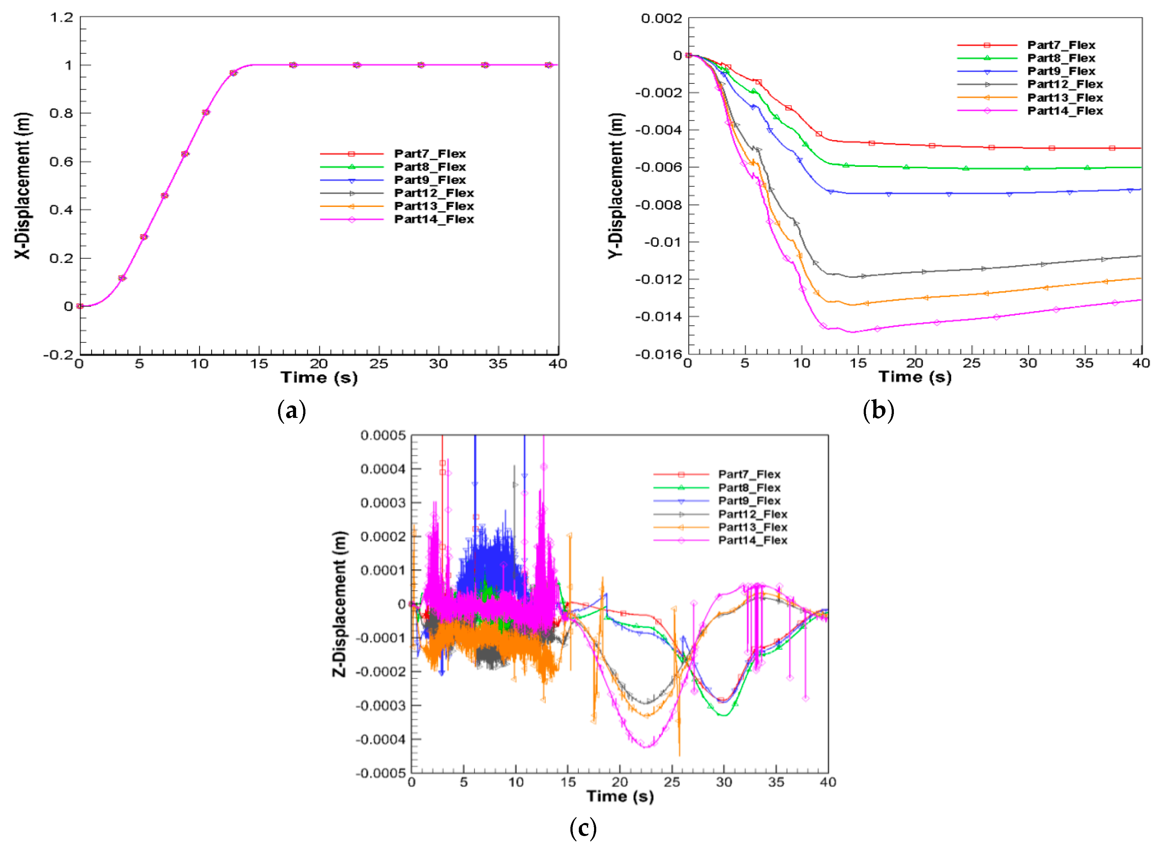
Kinematics and dynamic results are obtained from simulation experiments of the virtual flexible crawler system, in Figure 10. Figure 11 shows the time variation of the x, y and z displacements of front and middle flexible crawler shoes at equilibrium.

Table 4. Nodal locations of moved COM of flexible parts.

Location (m)	Part7_Flex	Part8_Flex	Part9_Flex	Part12_Flex	Part13_Flex	Part14_Flex
X	13.506	14.0696	14.7262	16.6988	17.3547	17.998
Y	9.2767	9.3308	9.3288	9.3338	9.3414	9.3386
Z	0.1958	0.2048	0.2112	0.2091	0.2027	0.2034

shows the x, y, z coordinates of the nearest nodal locations at time t = 0 (equilibrium). Both non-linear and linear crawler displacements are shown in the global x-direction (Figure 11a).

The x-displacement does not change during loading. Figure 11b shows that the crawler slides laterally in the negative y-direction during propel and slides in the opposite direction for loading. The lateral slide is due to oil sand deformation. The maximum lateral slide of 1.5 cm occurs for shoe 13 during propel. The z-displacement (Figure 11c) shows fluctuations with bouncing during propel. During loading, the displacement changes non-linearly due to non-linear semi-static loading conditions on crawler shoes. The sharp spikes in the z-displacement curve could be due to the friction between the crawler shoe and the edges of the connected oil sand units.

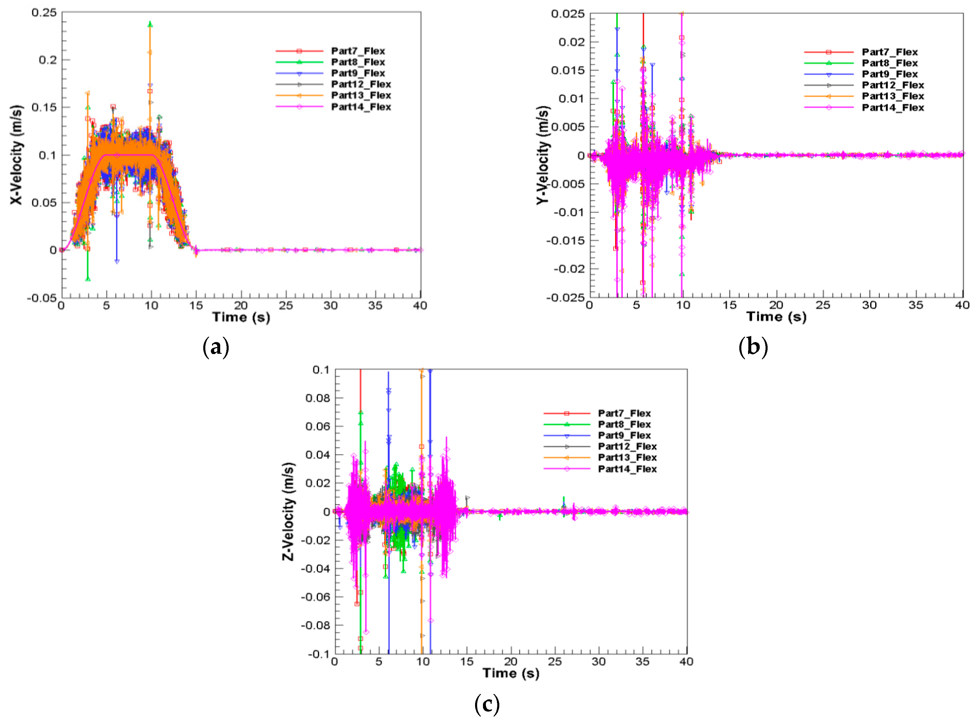
Figure 12 shows a time variation of x, y and z velocities for front and middle flexible shoes at the COM nodes. The x-velocity of shoe 13 (Figure 12a) follows Equation (1) and the other shoes are controlled by driver shoes via the joints. Figure 12b,c show that the y- and z-velocities vary during propel (0 < t < 15 s). The varying lateral sliding (y) velocity oscillates between ±0.01 m/s. The bouncing crawler z-velocity reaches a maximum during acceleration and deceleration with a maximum range between 0.05 and −0.085 m/s.

During constant velocity propel, the z-velocity fluctuates between 0.03 and −0.046 m/s. The x, y and z-velocities are negligible during loading between 15 < t < 40 s, as shown in Figure 12.

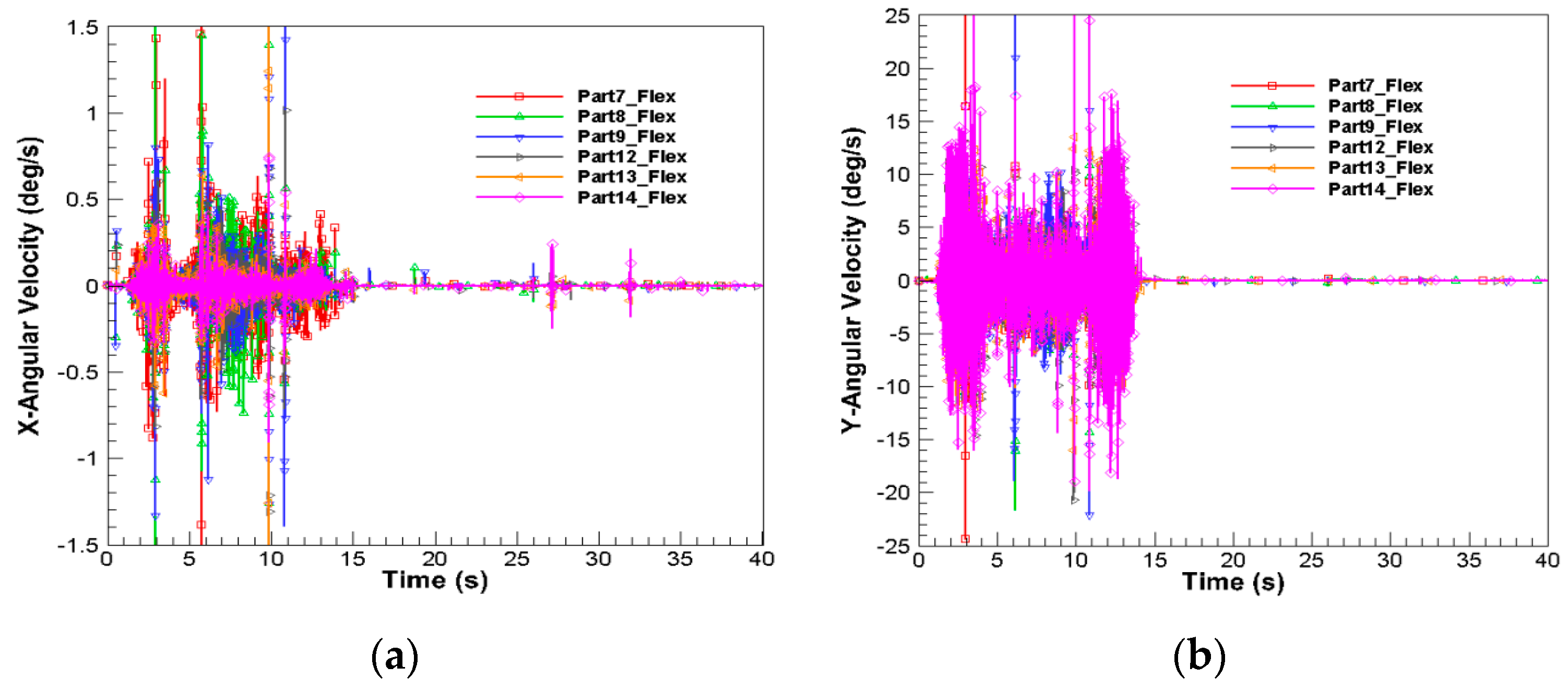
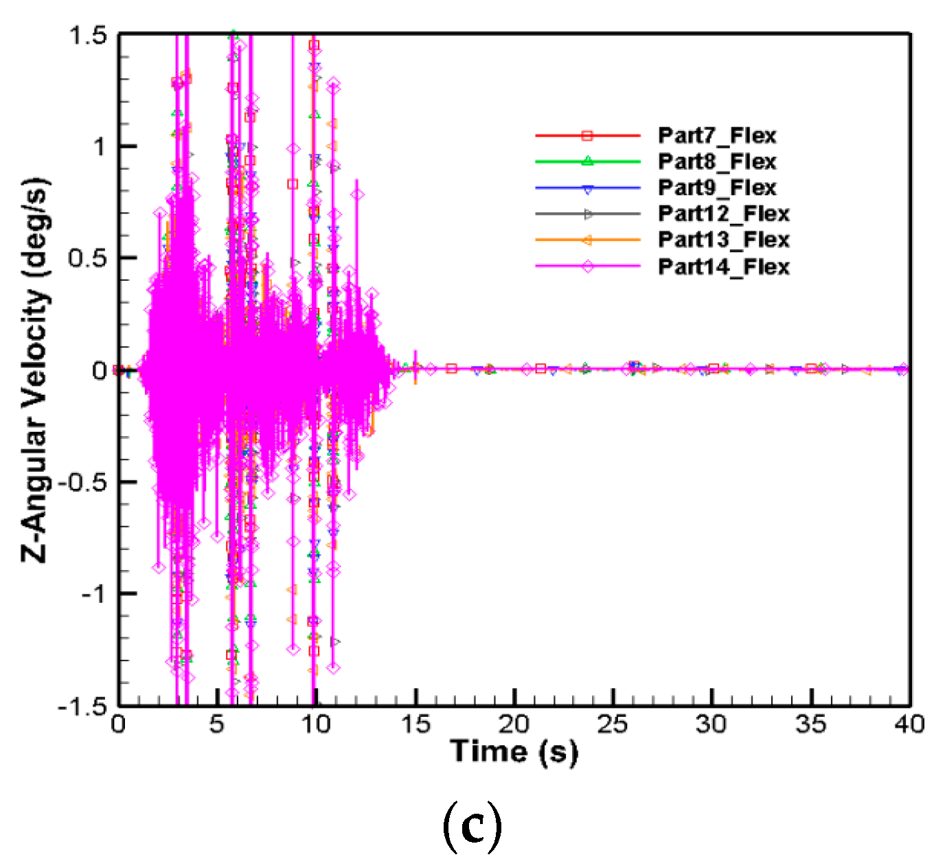
Figure 13 shows the angular velocities of crawler shoes about the global x, y and z directions. The crawler rolls with fluctuating x-angular velocity of ±0.5 deg/s, as in Figure 13a, during propel. Figure 13b shows that a large fluctuating angular velocity of ±15 deg/s develops around y-axis due to revolute joint between adjacent shoes. The crawler also rotates about the vertical z-axis with fluctuating velocity of ±0.5 deg/s in Figure 13c. The x, y and z angular velocities are negligible during loading (15 < t < 40 s), as in Figure 13.

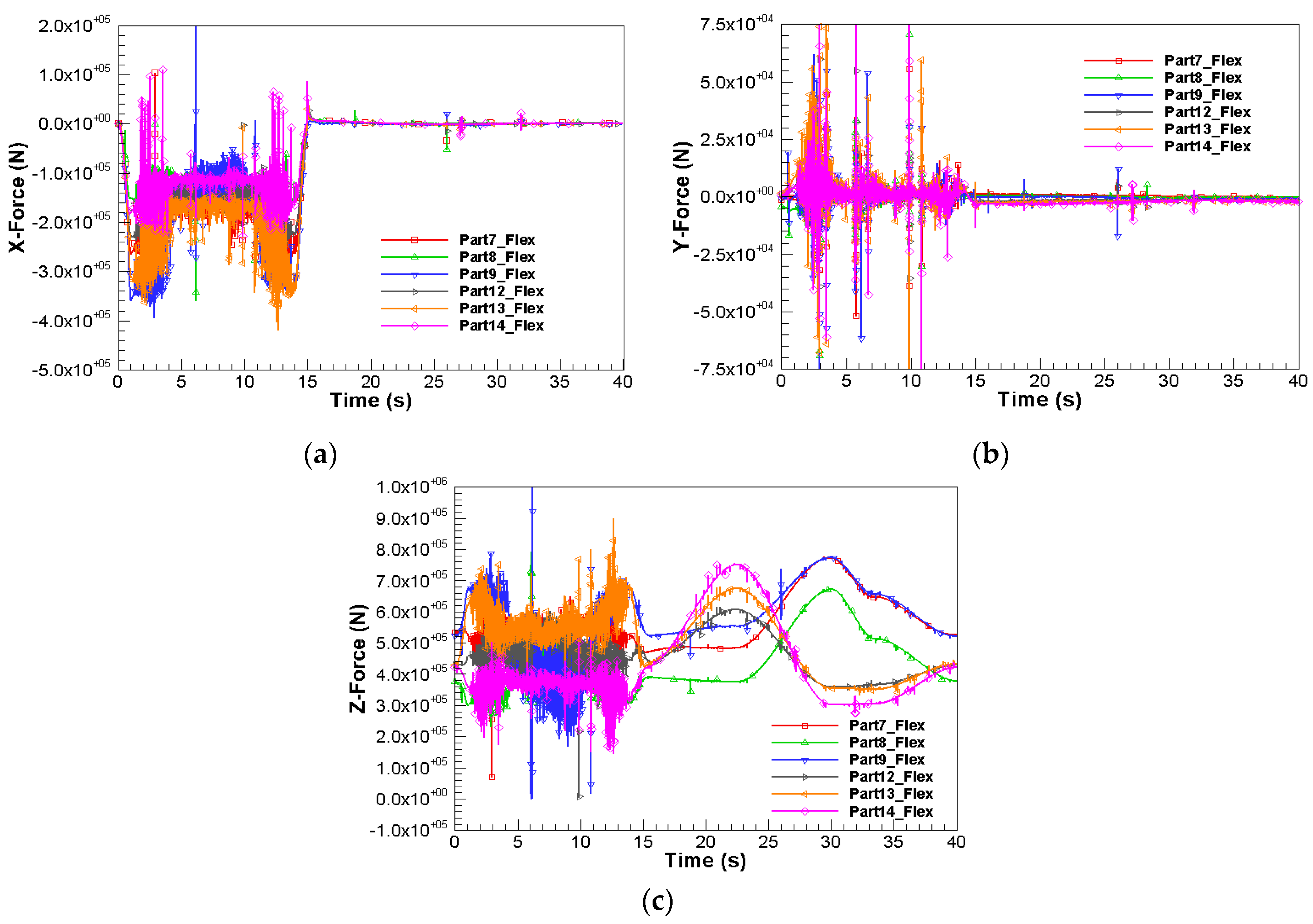
Figure 14 shows the total contact forces along x, y and z directions for each flexible shoe. The contact force in the x-direction (Figure 14a) is due to longitudinal propelling of the crawler. In the y-direction (Figure 14b), they are mainly due to lateral sliding of the crawler. The contact forces in the z-direction (Figure 14c) are due to normal crawler forces. The longitudinal (x) and lateral (y) forces are modeled using Coulomb friction force, and the normal (z) forces using the impact function in MSC ADAMS. Due to large fluctuations in slip velocity during acceleration and deceleration, the corresponding x-force fluctuations are also large. These fluctuations decrease during the constant velocity phase (Figure 14a). Figure 14a shows that the x-force fluctuates between 0 and −2.9758 × 10⁵ N during propel. The x-force during loading is negligible in comparison with propel and fluctuates between ±6000 N.

Similarly, the total y-force or lateral force (Figure 14b) fluctuates between 37,370 and −32,178 N during propel and during loading, there are negligible fluctuations between −1000 and −4000 N. The z-force variation (Figure 14c) shows large fluctuations between 7.7 × 10⁵ and 1.5 × 10⁵ N during propel, due to the bouncing motion of the crawler track in z-direction (Figure 11c). Since the z-position of crawler shoes changes due to the applied machine and dipper loads, the z-forces also vary non-linearly with time between 7.6 × 10⁵ and 3.0 × 10⁵ as in Figure 14c. The total torque applied on each crawler shoe due to the contact forces and frictional torque about the global x, y and z directions (not shown in Figure 14 due to space limitations) depend on x, y and z-contact forces. The total torque about x and y-axes depend on the z-force and, hence, their distribution is similar to z-force variation in Figure 14c. The z-torque depends on both the x and y contact forces.

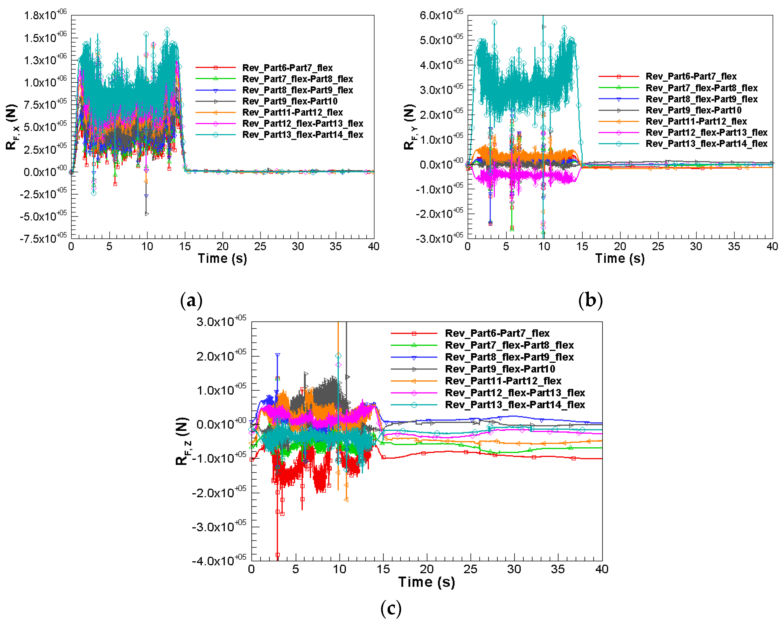
Since the y-force is an order of magnitude smaller than the x-force, the z-torque variation is similar to the x-force (Figure 14a). The maximum magnitude of x, y and z torques are 7 × 10⁶, 1.3 × 10⁷, and 3.7 × 10⁶ N·m, respectively, and are applied as external forces in Equation (4). Figure 15 shows the joint reaction forces at one of the two revolute joint constraints between rigid–flexible and flexible–flexible shoes, with similar forces at the other revolute joint. The reaction force in the x-direction (Figure 15a) is larger than that in the y and z-directions (Figure 15b,c). This is due to the applied motion constraint on flexible shoe 13, which pulls the crawler in the longitudinal direction to simulate shovel propel. The maximum x-reaction force is 1.5 × 10⁶ N in shoe 13 during acceleration and deceleration (Figure 15a). This motion constraint also causes a large reaction force in the y-direction in the joint connecting flexible parts 13 and 14, with a maximum value of 5 × 10⁵ N (Figure 15b). The y-reaction forces in the other joints are smaller, with a maximum value five times smaller than that between parts 13 and 14. The z-reaction force in the joints between the parts in Figure 15c is larger than the y-reaction force, with a maximum value of 2.5 × 10⁵ N. Figure 15c shows that, during loading, a large z-reaction force occurs at the joints, with negligible reaction forces in other directions.

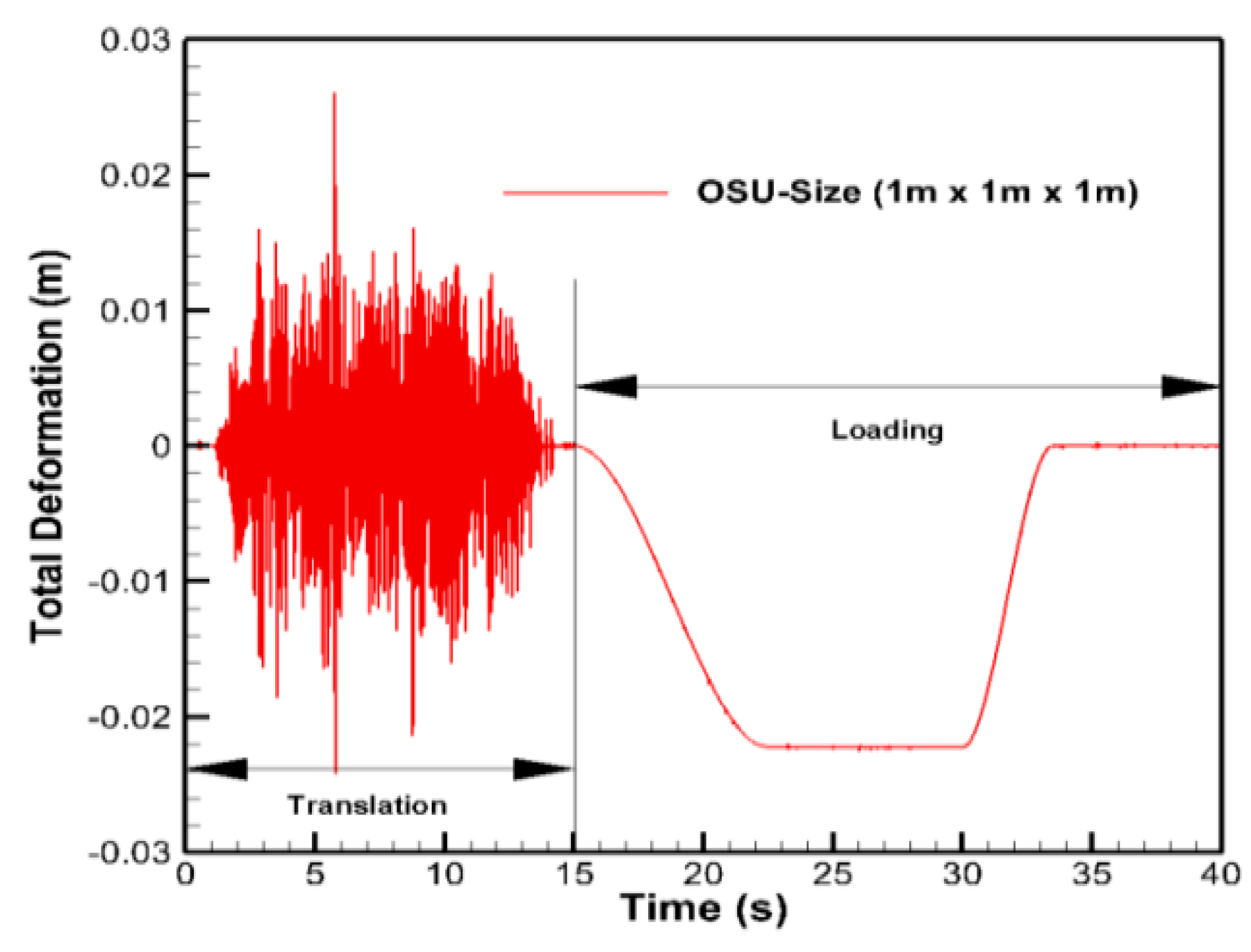
Large fluctuating reaction moments also occur at the joints about the global x and z directions during the propel motion. The maximum reaction torque about the x and z directions are 4 × 10⁴ N·m. The reaction torque about the y-direction is negligible since the crawler shoe is free to rotate in that direction. Figure 16 shows the oil sand deformation during propel and loading, which is the sum of the deformations in all the spring-damper oil sand units [17]. Large variations occur during propel with negligible variations for loading.

The propel and loading deformations range between −2.42 and 2.6 cm, and −2.25 and 0.023 cm, respectively. The largest deformation of 2.6 cm occurs during the constant velocity propel at time t = 5.76 s. The largest loading deformation of 2.25 cm occurs during swinging between 22.5 < t < 30 s.

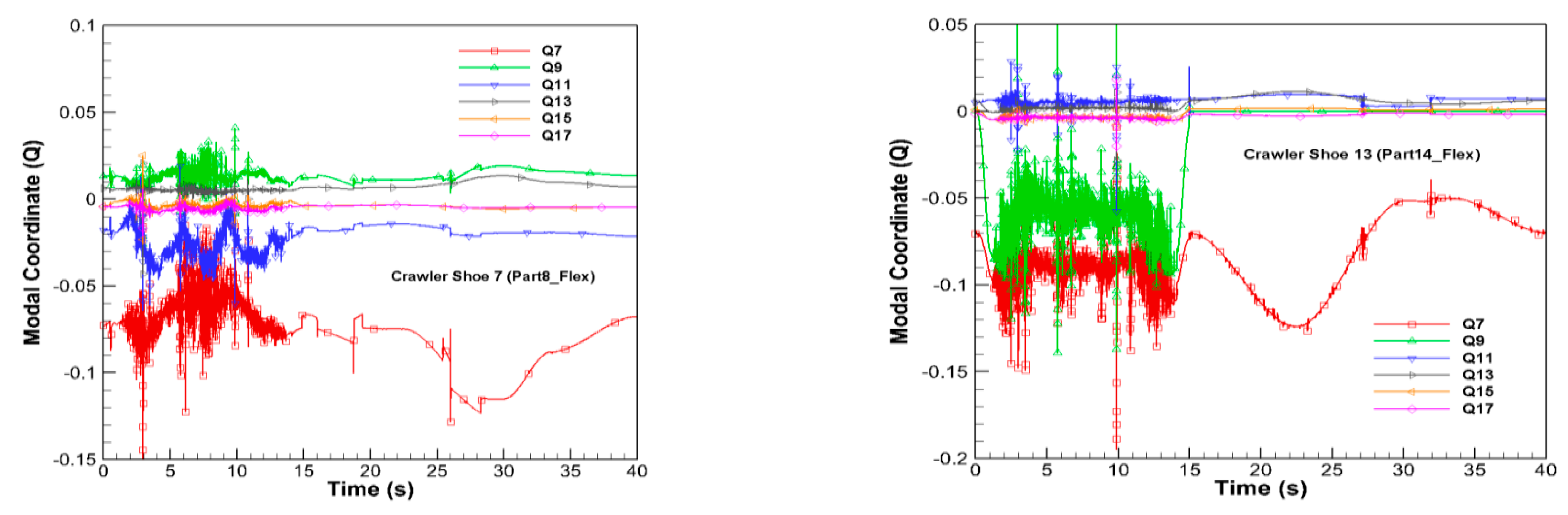
Figure 17 shows the time varying scale factors ($q$) in Equation (5) for mode shapes with frequencies within 0 < f < 1200 Hz for one of the flexible crawler shoes in the front set (shoe 13) and in the middle set (shoe 7) (Figure 10). The modal coordinate variation for other flexible shoes follows similar distribution. The contribution from mode shapes with frequencies greater than 1200 Hz is negligible. These modal coordinates are combined with modal stresses in MNF to obtain real time stress histories in the flexible crawler shoe.

During propel, the modal coordinates of all crawler shoes fluctuate but during loading they have a smooth non-linear semi-static variation. Figure 17 also shows that the modal coordinates for mode shape 7 is dominant with a maximum scale factor of 0.13. The discontinuity in the modal coordinates during loading in the solution could be due to a large integration error (E = 1 cm) in the ADAMS Solver.

5. Dynamic Stress Time Histories for Flexible Crawler Shoes

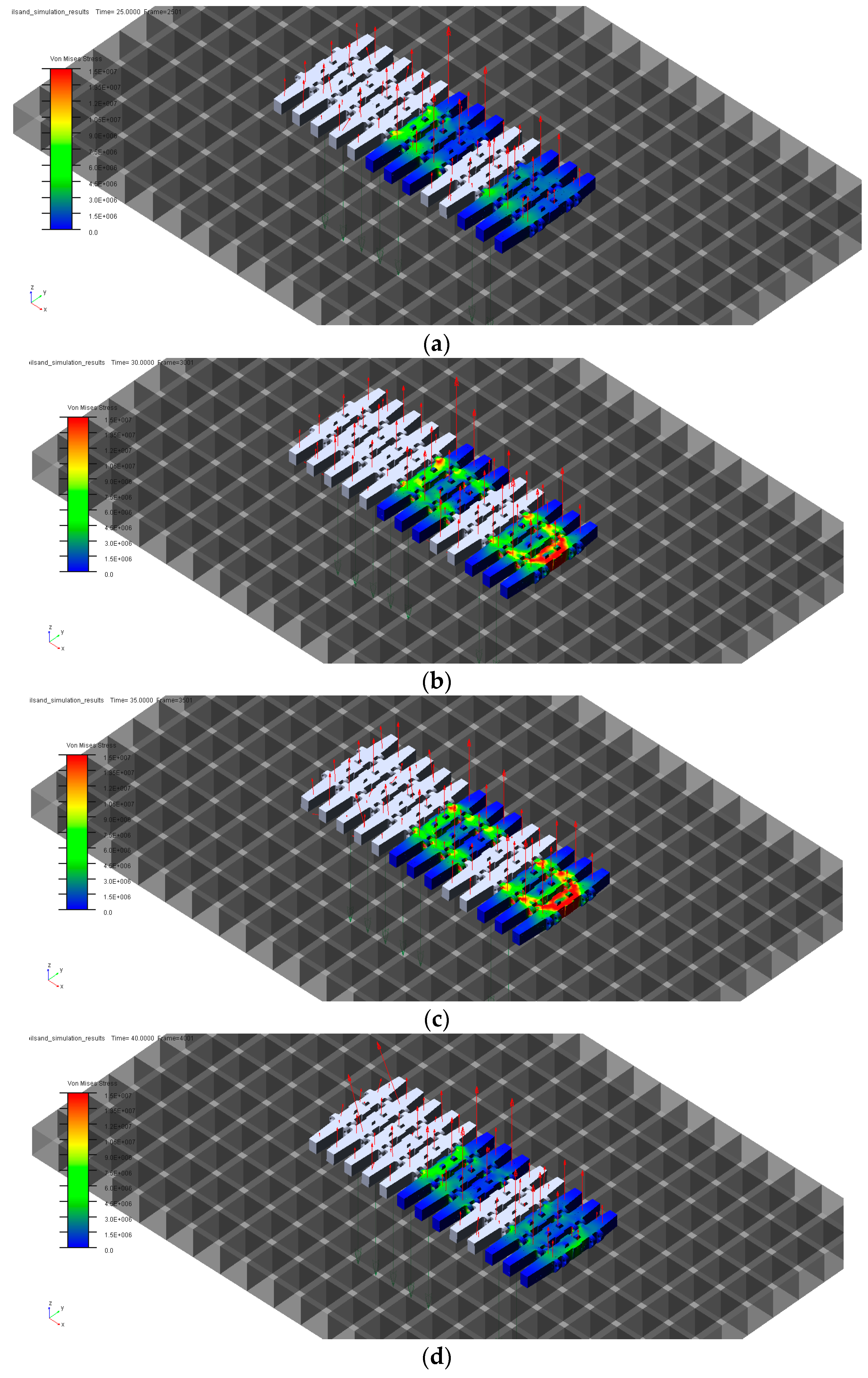
Figure 18 and Figure 19 show the von Mises stresses during propel and loading, at the beginning and end of shovel operation. The red arrows are contact forces on each crawler shoe, and the colored shoes show the von Mises stresses in N/m². Figure 18a shows the von-Mises stresses in the six flexible shoes at rest or at quasi-static equilibrium (t = 0). Even though the machine load is uniformly distributed, the middle crawler shoes are still subjected to a large amount of stress loading compared to the front crawler shoes. This is due to the uneven distribution of contact forces on each crawler shoe, as shown in Figure 18a. During acceleration (between 0 < t < 5 s), the front shoe stresses increase more rapidly than the middle shoes, as shown in Figure 18b.

During constant velocity propel (5 < t < 10 s), the high stress areas (≥1.5 × 107 N/m²) slightly increase in the middle and front crawler shoes, as shown in Figure 18c. These high stress areas further increase during part of the deceleration phase. About half a second before the end of deceleration phase (t ≈ 14.5 s), the high stress shoes start to decrease, and at t = 15 s, the crawler comes to rest, but can have free 6-DOF motion due to its interaction with the oil sands (Equation (1)). The stress crawler distribution (Figure 18d) returns approximately to the stress loading condition at rest (Figure 18a). Figure 18 shows that the stressed areas in driver crawler shoe 13 is much higher than those induced in the driven shoes during propel.

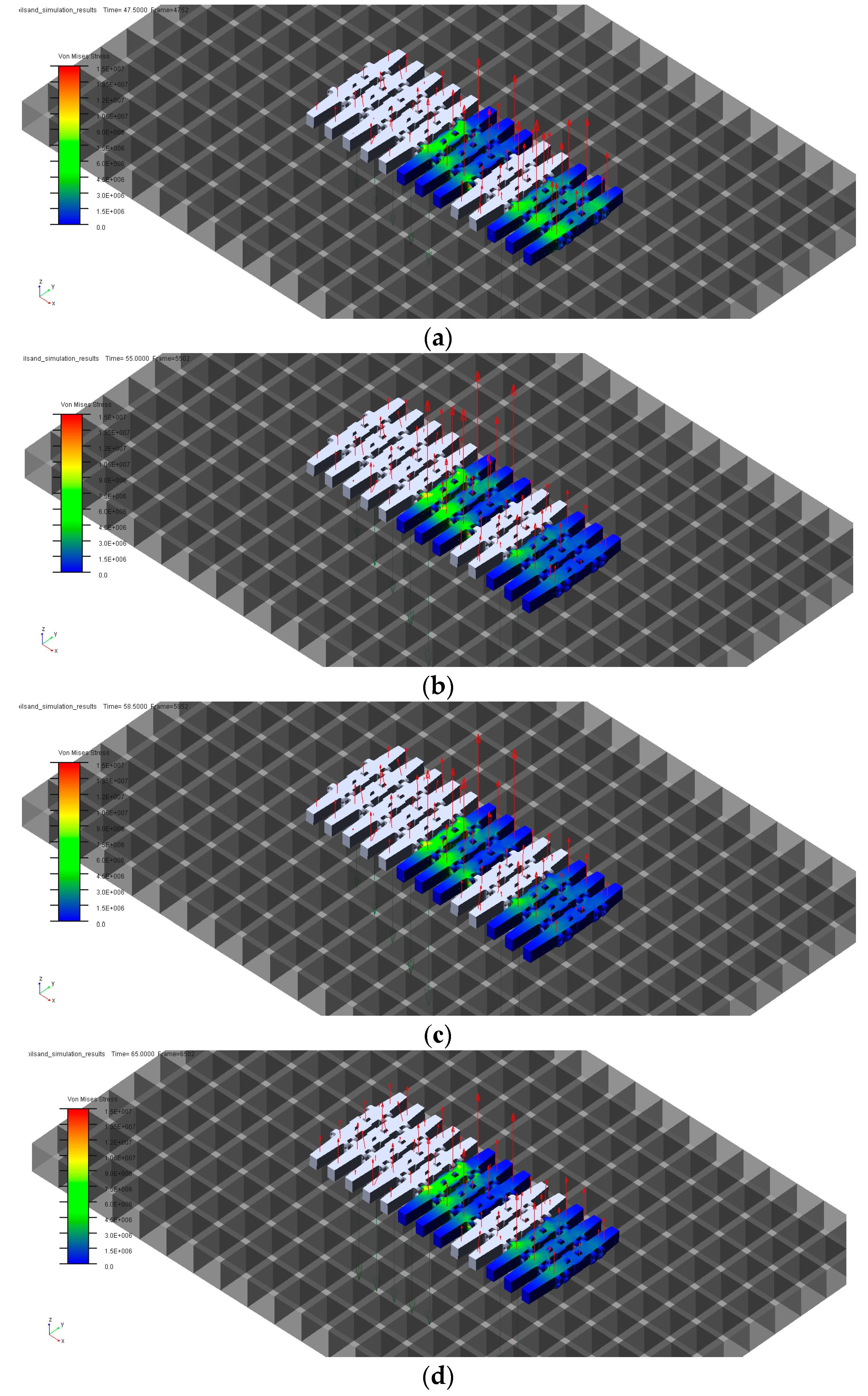
Figure 19 shows the crawler stress distribution during loading. During digging (15 < t < 22.5 s), the stresses increase in the front shoes and decrease in the middle shoes, as shown in Figure 19a. During swinging (22.5 < t < 30 s), the stresses steadily increase in the middle and decrease in the front, as shown in Figure 19b. Figure 19c shows that, during dumping (30 < t < 33.5 s), a small drop in stress is observed in the middle shoes, while a negligible change occurs in the front shoes. In the return phase (33.5 < t < 40 s), a slight decrease in stresses occurs in the middle shoes and increases in the front shoes at t = 40 s (Figure 19d). The stress loading returns to equilibrium at t = 0 s (Figure 18a). Figure 18 and Figure 19 show that the crawler stresses during loading are smaller than those during propel. This is due to the semi-static nature of the external applied load (Figure 6). The shovel is mostly stationary during loading, with a negligible shear motion or slip between the crawler and the ground. These conditions generate high normal forces (Figure 14c) with negligible tangential forces on crawler shoes (Figure 14a,b), resulting in low von-Mises stresses. The modal coordinate distribution in Figure 17 also shows that, during loading, only mode 7 (bending mode caused by normal force in Figure 9) contributes to stresses.

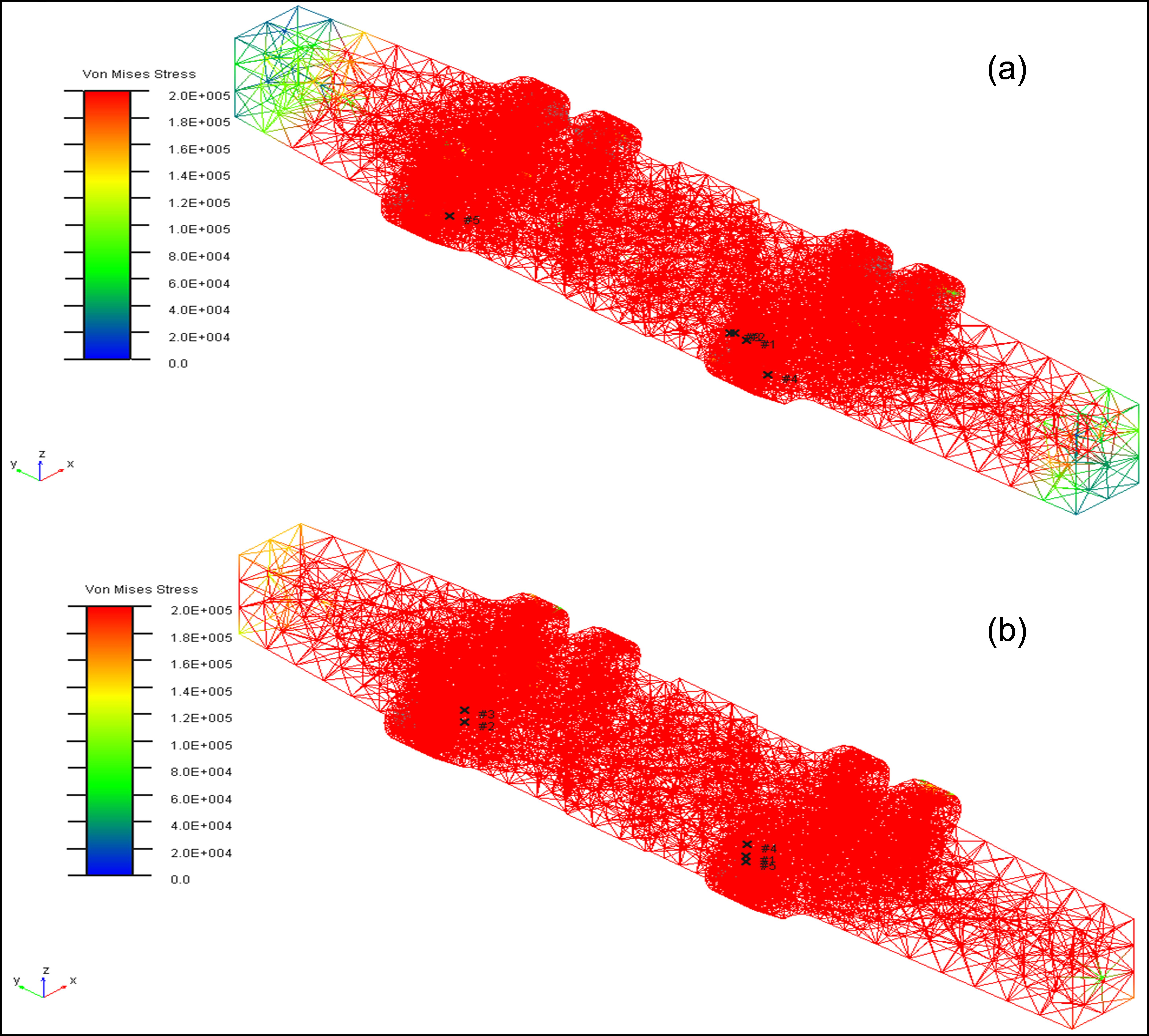
6. Hot Spots in the Flexible Crawler Shoes

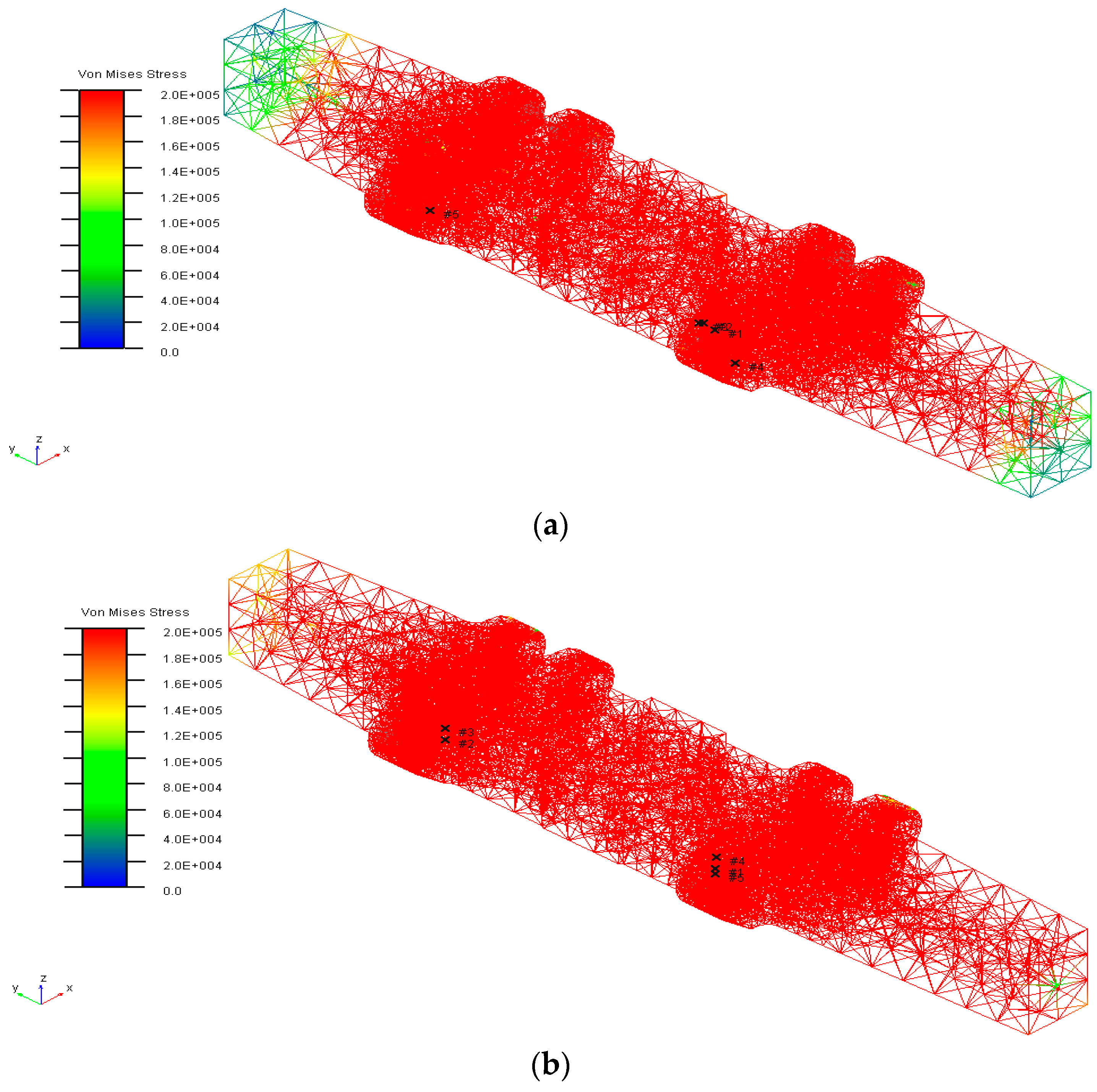
Figure 18 and Figure 19 show the general stress histories during the shovel operation. The maximum nodal stresses and their respective locations in the flexible shoes are extracted from MSC ADAMS/DURABILITY. Figure 20 shows the top five hot spots (highest nodal stress) for flexible shoes 7 and 13 (using marker “x”). The numbers after the marker “x” show the ranks of the stresses. The maximum contour value is 2 × 10⁵ N/m² for all the flexible bodies, as shown in Figure 20. The figure shows that all hotspots are located around the link pin joints, and not on the main crawler body.

However, the crawler shoe failure in the field mainly occurred in the roller path area, and not near the link pin regions from this study. The motion constraint (Equation (1)) on the shoe 13 COM node pulls the track through the joint connection between adjacent shoes. This causes a large amount of tension or joint reaction force in the x-direction (Figure 15a). This x-joint reaction force is responsible for the high stresses in the nodes around the link pin joint region (Figure 20). The hot spots information (von-Mises stress, node id, node location and time) for flexible shoes 7 and 13 are in

Table 5. Hot spot information for Part8_flex.

Hot Spots	Stress (MPa)	Node ID	Time (s)	Location
				x (m)	y (m)	z (m)
1	60.9882	29215	5.764	13.8622	8.59422	0.31395
2	60.5029	24820	5.764	13.7625	8.76	0.29596
3	60.3461	29214	5.764	13.8659	8.59198	0.26461
4	57.1899	24822	5.764	13.7415	8.76	0.31005
5	56.3833	29211	5.764	13.8677	8.59071	0.21533

and

Table 6. Hot spot information for Part14_flex.

Hot Spots	Stress (MPa)	Node ID	Time (s)	Location
				x (m)	y (m)	z (m)
1	172.1	26178	12.6803	17.749	8.76	0.22857
2	159.61	23866	12.6803	17.749	9.95	0.22858
3	158.541	23868	12.6803	17.749	9.95	0.28574
4	149.256	26176	12.6803	17.749	8.76	0.28573
5	144.916	26179	12.6803	17.749	8.76	0.19937

. The top five hot spots for other flexible shoes (6, 8, 11 and 12) are also located around the link pin joints.

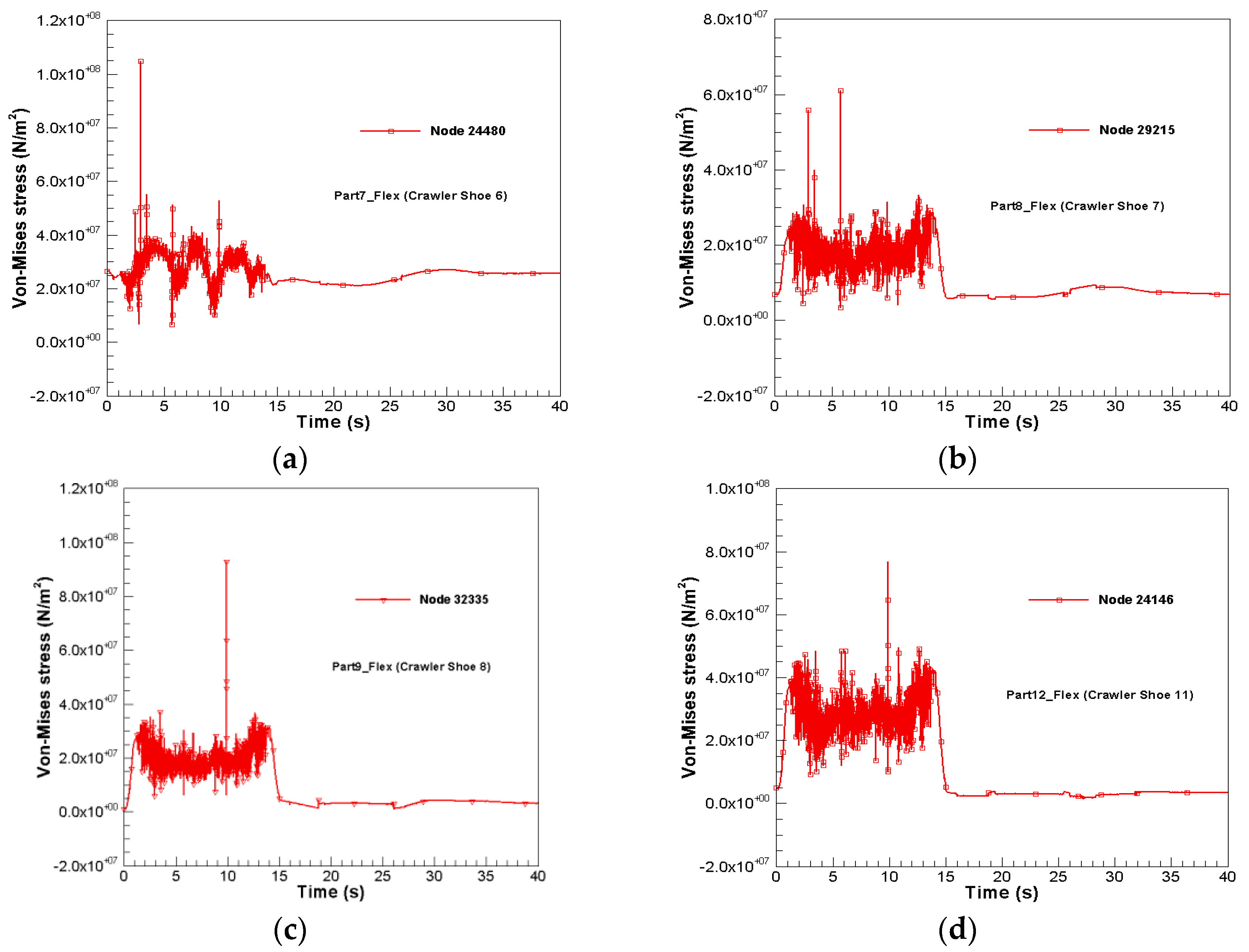
The time variation of von-Mises stresses for the highest nodal stresses (hot spot #1) for each part are shown in Figure 21. The maximum nodal stress on flexible Parts 7, 8, 9, 12, 13 and 14 are 53.6, 33.3, 37.07, 49.55, 103.33 and 172.1 MPa, respectively. Figure 21 shows that the maximum nodal stresses during propel follow the x-reaction force distribution in Figure 15a. Since x-reaction forces are larger on parts 14, 13 and 12 in comparison to parts 7, 8 and 9 (Figure 15a), the maximum nodal stresses are also larger on flexible parts 12, 13 and 14 (Figure 21d–f).

The yield strength of the A36 steel crawler material is 250 MPa [18]. Although the maximum nodal stresses in the shoes are smaller than the yield strength, the large fluctuating stresses during propel (Figure 21) can cause a shoe failure by fatigue due to crack initiation in the link pins. Although crawler shoes do experience tension or pulling forces when it passes over the rear idler or tumbler, field observation study undertaken at the Athabasca oil sand regions indicate that P&H 4100C BOSS crawler shoes develop cracks and break mainly at the roller path area, while the link pin joint lugs remained intact. The crushing force of the lower rollers, which distribute shovel weight along the crawler track [3], is responsible for this behavior and needs to be accounted for in the virtual prototype model to accurately predict the crawler shoe failure.

7. Conclusions

A 3D virtual prototype model of an open crawler track on oil sands terrain is developed in MSC ADAMS/FLEX/DURABILITY to capture crawler shoe stresses during propel and loading, using a rigid–flexible multi-body dynamics theory. The flexible shoes are generated from MNF using the Craig-Bampton theory on component mode synthesis and the dynamic solver in MSC NASTRAN. The load distribution on the crawler from machine weight and dipper payload is developed for propel and loading. The virtual model is simulated from quasi-static equilibrium for a period of 40 s. The propel motion consists of acceleration, constant velocity and deceleration phases for the first 15 s, and loading consists of digging, swinging, dumping and return for the remaining 25 s.

The kinematics simulation results show that the crawler track slides during shovel operation with a maximum displacement of 1.5 cm. During propel, the crawler velocities along the x, y and z directions fluctuate with a maximum of 0.15, 0.01 and 0.04 m/s, respectively. In addition, the crawler can also rotate about x-axis (roll) and z-axis (yaw) with a maximum value of ±0.5 deg/s. The dynamics simulation results show that, during propel, highly varying contact forces acts along x, y and z directions with maximum values of −2.9758 × 10⁵, 3.7 × 10⁴ and 7.7 × 10⁵ N, respectively. Large varying joint reaction forces develop along the x-direction with a maximum value of 1.5 × 10⁶ N in shoe 13. The distribution shows large stresses at the link pin region during propel. The maximum von Mises shoe stresses range between 33 and 172.1 MPa. The maximum nodal stress of 172.1 MPa occurs for crawler shoe 13 at node 26,178, located at the link pin region. The results also show that stress time histories during loading are semi-static, with a maximum stress of 27 MPa, which is far smaller than the corresponding maximum stress during propel.