Multi-Criteria Decision Making Approach for Hybrid Operation of Wind Farms

Abstract

Hybrid operation of wind farms has been in the limelight in recent years wherein the stochastic nature of wind causes market operators to choose an optimal strategy to maximize profit. The current work deals with a multi-criteria decision making approach to choose the best possible alternatives for a hybrid wind farm operation. A set of three, non-beneficial criteria, namely wind wakes, wind curtailment, and forced outages, were chosen to evaluate the best alternative. Three methods, (i) Simple Additive Weighting (SAW), (ii) the Technique for Order or Preference by Similarity to Ideal Solution (TOPSIS) and (iii) Complex Proportional Assessment (COPRAS), were applied to identify the best alternative, and the results revealed that for all three methods, borrowing deficit power from a neighboring wind farm is the best alternative. Comparative analyses in terms of the data requirement, the effect of dynamic decision matrices, and rank reversal in wind farm application have also been pioneered.

1. Introduction

Recently, alternative energy sources have gained much importance owing to their clean operation. With limited fossil fuel and nuclear resources, solar and wind energy technologies have outgrown their market share. Given its rich sustainability, a renewable energy power portfolio strengthens the backbone of a country’s economy [1]. Apart from its positive environmental impact, wind energy has also created job opportunities globally. With increased penetration of renewable energy sources, its operation and control has become important [2]. Wind turbines undergo a wide range of dynamic phenomenon. Achieving economies of scale is the primary objective for a wind farm operation. Given the random nature of wind speed, accurate wind forecasting schemes aid the operator to minimize the losses. However, the deficit power to the grid is fulfilled by a system of batteries operating at an investment cost. Selecting an optimum operational strategy lowers the system cost and increases the reliability of the power system.

Multi-Criteria Decision Making (MCDM) is a mathematical decision approach in order to select the best choices out of a given lot. The choices made out from these mathematical models may not always indicate the best “choice”. The MCDM approach can be divided into two prominent categories, that is outranking methods and compensatory methods. Compensatory methods involve choices that are more preferable owing to their positive attributes over negative ones, thus indicating a nominal trade off between the alternatives. Compensatory methods include Analytical Hierarchical Process (AHP) and Fuzzy Logic Decision Making (FLDM). Major applications of compensatory methods are in the field of water resources, like evaluation of rural water supply, resilience in water scarcity, and evaluation of desalination plants. On the other hand, outranking methods follow a sequence of logical decision making steps based on weights assigned to an individual criterion. Commonly-used outranking methods are the weighted sum and product method, the Technique for Order or Preference by Similarity to Ideal Solution (TOPSIS), the Complex Proportional Assessment (COPRAS) method, the Preference Ranking

Organization Method for Enrichment Evaluation (PROMETHEE), and Elimination Et Choix Traduisant la Realite Method (ELECTREE) [3]. However, the PROMETHEE method suffers from the problem of rank reversal, which may mislead the decision maker to choose the best alternatives when compared with other methods [4].

MCDM methods have been utilized across several science and engineering applications to select the best alternatives based on qualitative and quantitative information often collected via questionnaires and surveys. In the field of renewable energy, the MCDM methods have been successfully applied to energy planning, transportation energy management, utility planning, and building energy management [5]. Georgiou et al. have discussed AHP and PROMETHEE methods for selecting an efficient energy topology for a reverse osmosis desalination plant and have ranked five such topologies considering social, economical, and environmental impact [6]. Further, Kundakc et al. explored MCDM methods to select the best boiler for a dyehouse in the textile industry using two outranking methods, Measuring Attractiveness by a Categorical- Based Evaluation Technique (MACBETH) and Evaluation baseed on Distance from Average Solution (EDAS) [7]. Multi-criteria decision making is also used to select suitable wind turbines for developing a wind farm as explored by Lee et al. using Interpretive Structural Modeling (ISM) and the Fuzzy Analytical Hierarchical Process (FAHP) [8]. For each criterion, a sub-criterion is identified and a binary matrix indicating the relationship between them is created. Mahdy et al. have identified the offshore wind energy potential in Egypt using the Geographical Information System (GIS)-based AHP technique where several factors like wind, water depth, and distance from shore were considered [9]. In terms of selecting offshore turbine structures, Kolios et al. have studied the MCDM approach under stochastic inputs where factors like environmental impact, depth compatibility, cost of installation, and maintenance cost were considered as criteria [10]. Al Garni et al. discussed the MCDM approach for evaluating renewable power sources for Saudi Arabia where the AHP method was used, and the results revealed that solar PV technology is more preferred followed by solar thermal technology [11]. Several criteria like environmental, socio-cultural, and political impact were considered. The effect of the normalization of beneficial and non-beneficial criteria also influences the selection process. Jahan et al. have presented a comprehensive review of normalization techniques used for streamlining the decision making process [12].

The most important purpose of adopting any MCDM approach is to translate the performances of each alternative into a single aggregated value to smooth the progress of the ranking process. Since no solo mode of analysis is adequate to deal with the different types of complex decision making problems, as well as there is no distinct aggregation method that is unanimously acceptable for any kind of decision problem, the Decision Makers (DMs) have to select the method based on the characteristics of the problem and the information available. Analyzing the above-mentioned prospects, this paper aims at applying some multi-beneficial MCDM methods that can make the decision making process trouble free and to be well suited to most of the situations. The major contribution of this paper is the application of several MCDM methods for hybrid operation of a wind farm considering dynamic phenomena like wind wakes, wind curtailment, and forced outage of turbine unit(s). Meanwhile, we also present four alternatives amongst which the best one is to be selected. The MCDM approach was carried out using Simple Additive Weighting (SAW), TOPSIS, and the COPRAS method. The cumulative priority scores for each alternative were determined, and the ranking was validated for two wind datasets.

This paper is organized as follows: Section 2 discusses the problem formulation for the hybrid operation of a wind farm where the alternatives are described in detail. Section 3 sheds light on the MCDM techniques used along with a step-by-step procedure, followed by the results and a discussion in Section 4. A comparative analysis of the different MCDM techniques is then presented in Section 5, followed by the concluding remarks in Section 6.

2. Problem Formulation

A wind farm’s secure and reliable operation is dependent on the availability of wind resource. Wind speed density and wind direction for a given terrain play a significant role in maximizing power capture. With advanced manufacturing technologies and the availability of automation, the production costs for a wind turbine have lowered in the past decade [13]. Apart from the wind resource, complex terrains add a significant problem to the turbine siting process where the irregular land and scanty resources increase transportation and labor cost significantly. Hence, an accurate wind forecast schedule seems to compensate the disadvantages posed by initial installation processes. A wind farm operator must submit a power schedule ahead of time as a part of an agreement with the utility grid. The random nature of wind speed leads to errors in forecasting, and thus, there exist events of surplus and deficit power. The current problem of economic operation that deals with the events of surplus and deficit power is handled by Battery Energy Storage Systems (BESS). The accuracy of wind forecasting techniques influences the charging or discharging schedule of the BESS. For wind power applications, commonly-used BESS include lithium-ion, lead-acid and nickel-cadmium batteries. Patel et al. have discussed several methodologies to achieve optimized hybrid wind power generation, and we extend these four alternatives to solve the MCDM problem for a wind farm [14].

• Alternative 1 ($A_1$): Let ${\widehat{p}}_i$ represent the forecasted wind power in a particular forecast window and $p_i$ be the actual wind power from the wind farm. In scenarios where ${\widehat{p}}_i$ is greater than $p_i$, a penalty is paid for the deficit power by the wind farm operator, and the battery bank is left unused. The total cost paid by the operator in such k instances is given as:

  $$\begin{array}{ccc}\hfill F_1& =& \beta \sum _{i=1}^k\left({\widehat{p}}_i-p_i\right),\hfill \end{array}$$

  (1)

  where $\beta$ represents the penalty cost ($) per 1 kW of deficit power. However, no penalty is to be paid if $p_i>{\widehat{p}}_i$.
• Alternative 2 ($A_2$): In this alternative, the deficit power is fed to the grid via a combination of two strategies. Firstly, a threshold battery power ($p_b^{th}$) is identified, and if the deficit (${\widehat{p}}_i-p_i$) is greater than the threshold, the penalty is paid for the said difference. The total cost paid by the operator during such m instances is given as:

  $$\begin{array}{c}\hfill F_2=\zeta \sum _{i=1}^m\left(p_{bi}^{th}-{\widehat{p}}_i+p_i\right),\end{array}$$

  (2)

  where $\zeta$ is the penalty cost (in $/kW) for violating the battery threshold limit.
• Alternative 3 ($A_3$): In this alternative, the deficit wind power is pumped into the grid by neighboring wind farms, and the penalty for the said difference is paid by the wind farm operator. Suppose the actual and forecasted wind powers for Wind Farms 2 and 3 are $p_{2i}$, ${\widehat{p}}_{2i}$, $p_{3i}$ and ${\widehat{p}}_{3i}$ respectively, then the penalty cost paid by the operator of Wind Farm 1 is given as:

  $$\begin{array}{c}\hfill F_3=\left\{\begin{array}{c}\alpha \sum _{i=1}^l(p_{2i}-{\widehat{p}}_{2i}),\mathrm{if}{p}_{2i}>{\widehat{p}}_{2i},\hfill \\ \alpha \sum _{i=1}^l(p_{3i}-{\widehat{p}}_{3i}),\mathrm{if}{p}_{3i}>{\widehat{p}}_{3i},\hfill \\ \delta \sum _{i=1}^l(\widehat{p_i}-p_i),\hfill \end{array}\right.\end{array}$$

  (3)

  where $\alpha$ and $\delta$ represent the penalty cost and the cost of using the battery to compensate 1 kW of deficit power, respectively. It must be noted that the penalty cost of using the battery in this methodology is higher than the penalty cost in Alternatives 1 and 2.
• Alternative 4 ($A_4$): In this case, the entire deficit power is delivered by the battery bank, and the cost paid by the operator in u such instances is given as:

  $$\begin{array}{c}\hfill F_4=\delta \sum _{i=1}^u({\widehat{p}}_i-p_i),\end{array}$$

  (4)

  where $\delta$ represents the penalty cost paid by the wind operator to compensate 1 kW of wind power deficit entirely by battery.

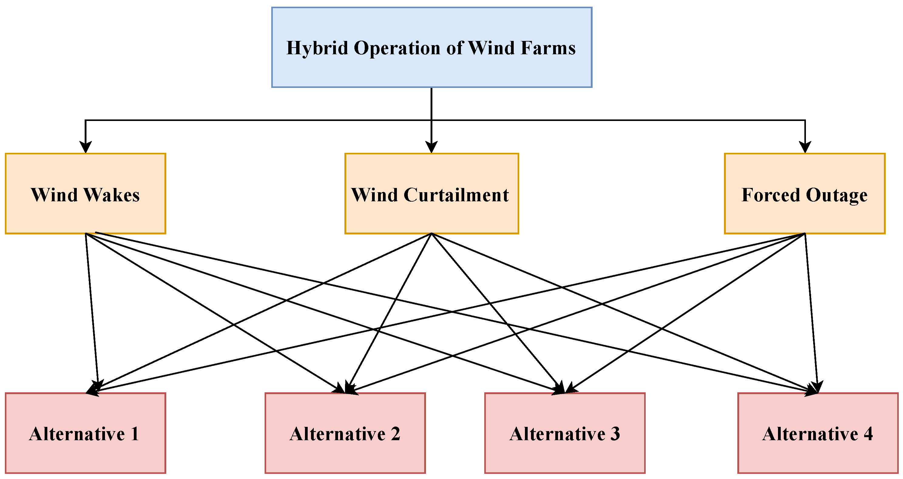
Based on the four alternatives discussed, we now shall assess the criteria under which the said MCDM problem is to be evaluated. For a wind farm operating in the Prandtl layer (extending up to 100 m), wind wake is a common aerodynamic phenomenon causing reduced power production for downwind turbines. Power loss due to wind wakes can be compensated by either of the four alternatives discussed previously. Similarly, wind curtailment due to generating system limitations is a common phenomenon as well, where dealing with surplus power is an important task. Henriot discussed the economic impact of power curtailment in the case of renewable energy sources with thermal generators [15]. Wind curtailment can be positively dealt with using one of the aforementioned alternatives. Apart from that, forced outage in a wind farm occurs when a turbine unit is to be drawn out for cleaning or maintenance purposes and disturbs the forecasted power schedule simultaneously calling the need for deficit power from any one of the stated methodologies.

Furthermore, wind farm operation is also governed by its surroundings in terms of quality of the landscape. Landscape quality has been assessed over the years by using several qualitative and quantitative indicators. The socioeconomic impacts of wind turbine commissioning have led to critical study of landscape quality. Recently, a cost action report titled “Renewable Energy and Landscape quality” was analyzed thoroughly, which investigated the relationship between the potential renewable energy sources and landscape quality [16]. In the present case, the four alternatives describing different proportions of usage for the penalty and battery have direct and indirect impacts on the landscape quality of wind farms. In the case of hybrid operation perceived by a system of batteries, the pollution caused due to lead or any other harmful chemical can degrade the ecological functioning of the site. However, with the advancement in manufacturing and material design, the harmful effects can be controlled to preserve the landscape quality. While it is worth to noting that all the wind farms considered had the same number of wind turbines, in the case of a different number of turbines, the effect on landscape quality would be different. With a lesser number of wind turbines and a greater number of battery units, the damage caused due to emissions to the ecosystem would be more pronounced. Another issue with wind turbines is the problem of noise emission. Noise generated from wind turbines is mainly categorized as mechanical and aerodynamic noise. The mechanical noise is mainly due to the gearbox and generator section, while the aerodynamic noise is mainly due to ambient turbulence or wake-generated turbulence. Several empirical models exist that trace the relationship between global emitted noise and wind turbine parameters. According to Lowson [17], the emitted noise in dB is given as:

$$\begin{array}{c}\hfill L_{WA}=22{\log }_{10}D+72,\end{array}$$

(5)

where D is the rotor diameter. Thus, the increase in the emitted noise level would certainly impact the livelihood of persons surrounding the wind turbine and would pose a barrier to accepting wind energy in promising areas.

Table 1. Criteria for the MCDM approach.

Label	Criteria	Summary
$C_1$	Wind wakes	Cause power reduction
$C_2$	Wind curtailment	Surplus power either fed to battery or used as power loan
$C_3$	Forced outage	Reduces wind farm capacity

discusses the criteria used for the said MCDM problem and Figure 1 illustrates the schematic representation of MCDM process.

3. MCDM: Materials and Methods

The MCDM approach helps decision makers to identify the best alternatives given that there exists an array of plausible criteria to justify the choice. An MCDM problem may be formulated in the form of an $m\times n$ matrix where the matrix element, say $h_{ij}$, describes a semantic relationship between the alternative i w.r.t the criteria j. Such a decision matrix can be expressed as:

$$H=\begin{array}{cc}\begin{array}{cccc}{C}_1& C_2& \cdots & C_n\end{array}& \\ \left(\begin{array}{cccc}{h}_{11}& h_{12}& \cdots & h_{1j}\\ h_{21}& h_{22}& \cdots & h_{2j}\\ ⋮& ⋮& ⋮& ⋮\\ h_{i1}& \cdots & \cdots & h_{ij}\end{array}\right)& \begin{array}{c}{A}_1\\ A_2\\ ⋮\\ A_m\end{array}\end{array}$$

In the above matrix H, $h_{ij}$ is for $i=1,2,\dots ,m$ and $j=1,2,\dots ,n$, which represents the performance score for the alternative i w.r.t. the criterion j. In the present work, we approach the decision making problem through three methods: (i) Simple Additive Weighting (SAW), (ii) the Technique for Order or Preference by Similarity to Ideal Solution (TOPSIS), and (iii) the Complex Proportional Assessment (COPRAS) method. We now describe these methods in brief and how they provide the best solution.

3.1. Simple Additive Weighting (Saw) Method

Hwang et al. in 1981 devised a method to solve the MCDM problem by assigning each performance score of alternative $A_i$ with a specific weight $w_i$, and a weighted sum of all the criteria for a particular alternative is obtained [18]. The step-by-step procedure for the SAW method can be described as:

• Step 1: Identify the alternatives ($A_1,A_2,\dots ,A_m$) and criteria ($C_1,C_2,\dots ,C_n$) for the decision making problem.
• Step 2: Develop a decision matrix for the said MCDM problem.
• Step 3: Construct the normalized decision matrix with its elements as:

  $$\begin{array}{c}\hfill \widehat{H_{ij}}=\frac{\min h_{ij}}{h_{ij}}i=1,2,\dots ,m;j=1,2,\dots ,n.\end{array}$$

  (6)

  $$\begin{array}{c}\hfill \widehat{H_{ij}}=\frac{h_{ij}}{\max h_{ij}}i=1,2,\dots ,m;j=1,2,\dots ,n.\end{array}$$

  (7)
  For non-beneficial criteria, the normalized element of the decision matrix is calculated using Equation (6) and for beneficial criteria using Equation (7).
• Step 4: Calculate entropy ($e_j$) and divergence values ($d_j$) for each criteria as:

  $$\begin{array}{ccc}\hfill e_j& =& -\frac{1}{\log m}\sum _{i=1}^m\widehat{H_{ij}}\log (\widehat{H_{ij}}).\hfill \end{array}$$

  (8)

  $$\begin{array}{ccc}\hfill d_j& =& |1-e_j|j=1,2,\dots ,n.\hfill \end{array}$$

  (9)
• Step 5: Calculate the weights for the respective criterion using Equation (10):

  $$w_j=\frac{d_j}{{\sum }_{j=1}^n{d}_j}.$$

  (10)
• Step 6: Finally, calculate the priority score for each alternative using Equation (10) and arrange them according to highest priority:

  $$\begin{array}{c}\hfill S_i=\sum _{j=1}^n{w}_j{h}_{ij}.\end{array}$$

  (11)

3.2. Technique for Order or Preference by Similarity to Ideal Solution Method

The technique for Order or Preference by Similarity to Ideal Solution (TOPSIS) selects the best choice based on the shortest Euclidean distance to the positive ideal solution and the longest distance to the negative ideal solution [19]. Lourenzutti et al. have proposed a generalized TOPSIS method where multiple decision makers have the power to define their own set of criteria, weights, and factors affecting alternatives, and it was validated for three different case studies [20]. Balioti et al. explored the TOPSIS method to select an optimal spillway design for a dam site in North Greece [21]. Here, five spillway designs were treated as alternatives, and nine design criteria were assessed under a fuzzy environment, whereas the AHP method was used to assign weights to the criteria. The following steps were used to evaluate the priority score:

• Follow Steps 1–2 as in the case of the SAW method.
• Construct the normalized decision matrix with its elements as:

  $$\begin{array}{c}\hfill \widehat{H_{ij}}=\frac{h_{ij}}{\sqrt{{\sum }_{j=1}^n{h}_{ij}^2}}i=1,2,\dots ,m;j=1,2,\dots ,n.\end{array}$$

  (12)
• After calculating weights for each criterion, construct a weighted normalized matrix:

  $$\widehat{h}=w_j{H}_{ij};i=1,2,\dots ,m;j=1,2,\dots ,n.$$

  (13)
• Identify positive and negative ideal solutions $S^{+}$ and $S^{-}$ respectively as:

  $$\begin{array}{cc}\hfill S_j^{+}& =\{\left(\max h_{ij}\right|j\in t);\left(\min h_{ij}\right|j\in n-t)|i=1,2,\dots ,m\},\end{array}$$

  (14)

  $$\begin{array}{cc}\hfill S_j^{-}& =\{\left(\min h_{ij}\right|j\in t);\left(\max h_{ij}\right|j\in n-t)|i=1,2,\dots ,m\},\end{array}$$

  (15)

  where t represents the number of beneficial criteria and $n-t$ the non-beneficial criteria.
• The p-norm Euclidean distances $D_i^{+}$ and $D_i^{-}$ are determined as:

  $$\begin{array}{ccc}\hfill D_i^{+}& =& {\left\{\sum _{j=1}^n{\left({\widehat{h}}_{ij}-S_j^{+}\right)}^p\right\}}^{1/p}i=1,2,\dots ,m;j=1,2,\dots ,n.\hfill \end{array}$$

  (16)

  $$\begin{array}{ccc}\hfill D_i^{-}& =& {\left\{\sum _{j=1}^n{\left({\widehat{h}}_{ij}-S_j^{-}\right)}^p\right\}}^{1/p}i=1,2,\dots ,m;j=1,2,\dots ,n.\hfill \end{array}$$

  (17)
• Evaluate the relative closeness of each alternative using Equation (18) and rank them in descending order:

  $$G_i=\frac{D_i^{-}}{D_i^{-}+D_i^{+}}i=1,2,\dots ,m;0\le G_i\le 1.$$

  (18)

3.3. Complex Proportional Assessment (Copras) Method

The COPRAS method implements a stepwise ranking procedure to assess the performance of each alternative considering conflicting situations. Zolfani et al. implemented COPRAS and AHP to solve the supplier selection problem with time, cost, quality, and service as key factors [22]. Bhowmik et al. implemented the entropy-based COPRAS method to solve the problem of selecting an appropriate green energy source for the region of Tripura, India [23]. Hydro, solar, biomass, and biogas were chosen as the possible alternatives based on a set of beneficial and non-beneficial criteria. The COPRAS method is based on the following steps:

• Construct a hierarchy model for the said MCDM problem.
• Arrive at constructing the normalized decision matrix and determine the weights associated with each criterion as calculated in the case of the TOPSIS method.
• Determine weighted normalized matrix $\widehat{H_{ij}}$ using Equation (12).
• Determine the sum of weighted scores for beneficial and non-beneficial criteria using:

  $$\begin{array}{ccc}\hfill R_i^{+}& =& \sum _{j=1}^t{\widehat{h}}_{ij},R_i^{-}=\sum _{j=t+1}^n{\widehat{h}}_{ij}|i=1,2,\dots ,m,\hfill \end{array}$$

  (19)

  where t represents the number of beneficial criteria and $n-t$ the non-beneficial criteria.
• Determine relative priorities for each alternative as:

  $$\begin{array}{c}\hfill U_i=R_i^{+}+\frac{{\sum }_{i=1}^m{R}_i^{+}}{R_i^{-}{\sum }_{i=1}^m\frac{1}{R_i^{-}}}.\end{array}$$

  (20)
• Arrive at the final priority score for each alternative and arrange them in descending order:

  $$L_i=\frac{U_i}{U_{max}}\times 100\%.$$

  (21)

4. Results and Discussion

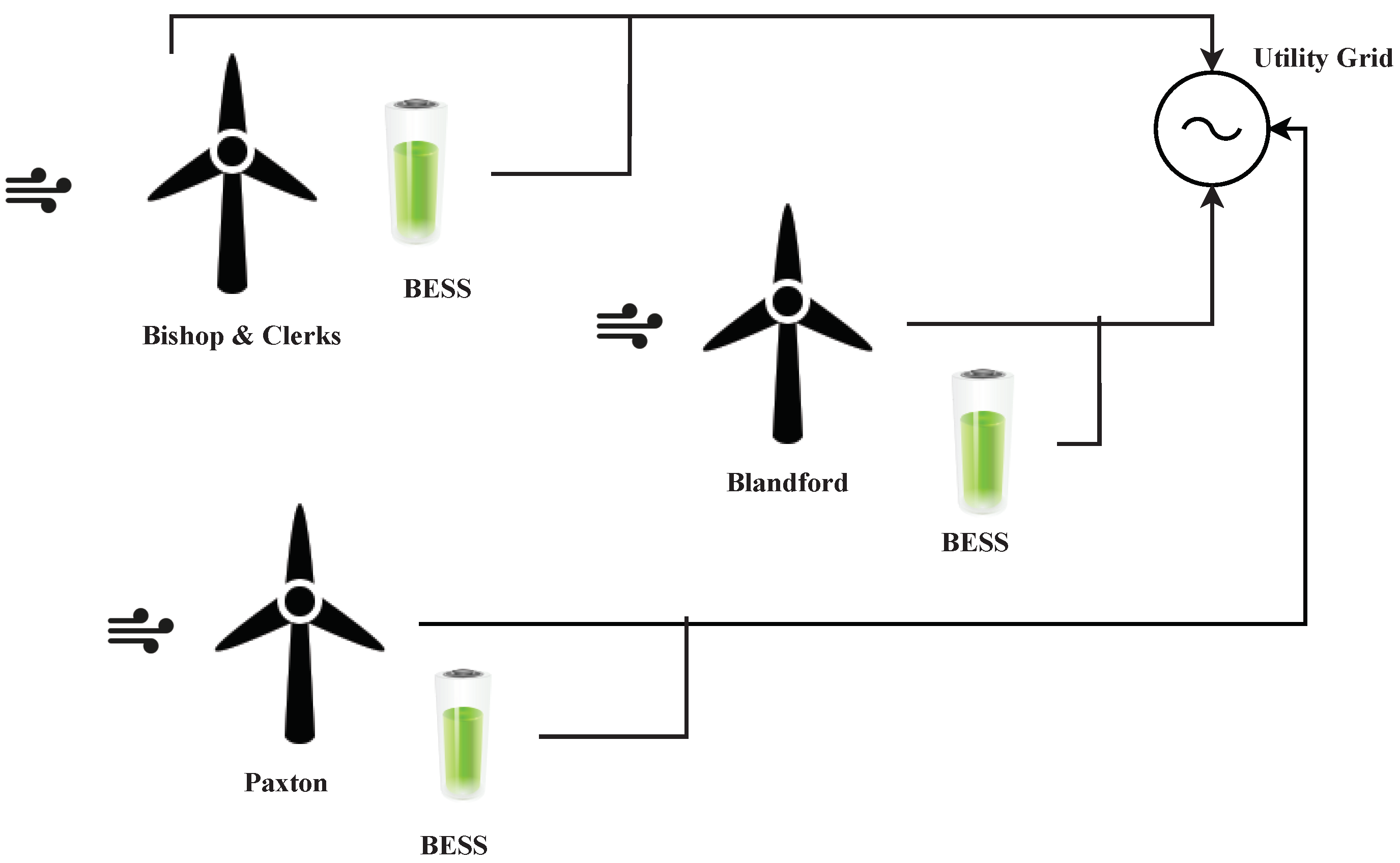
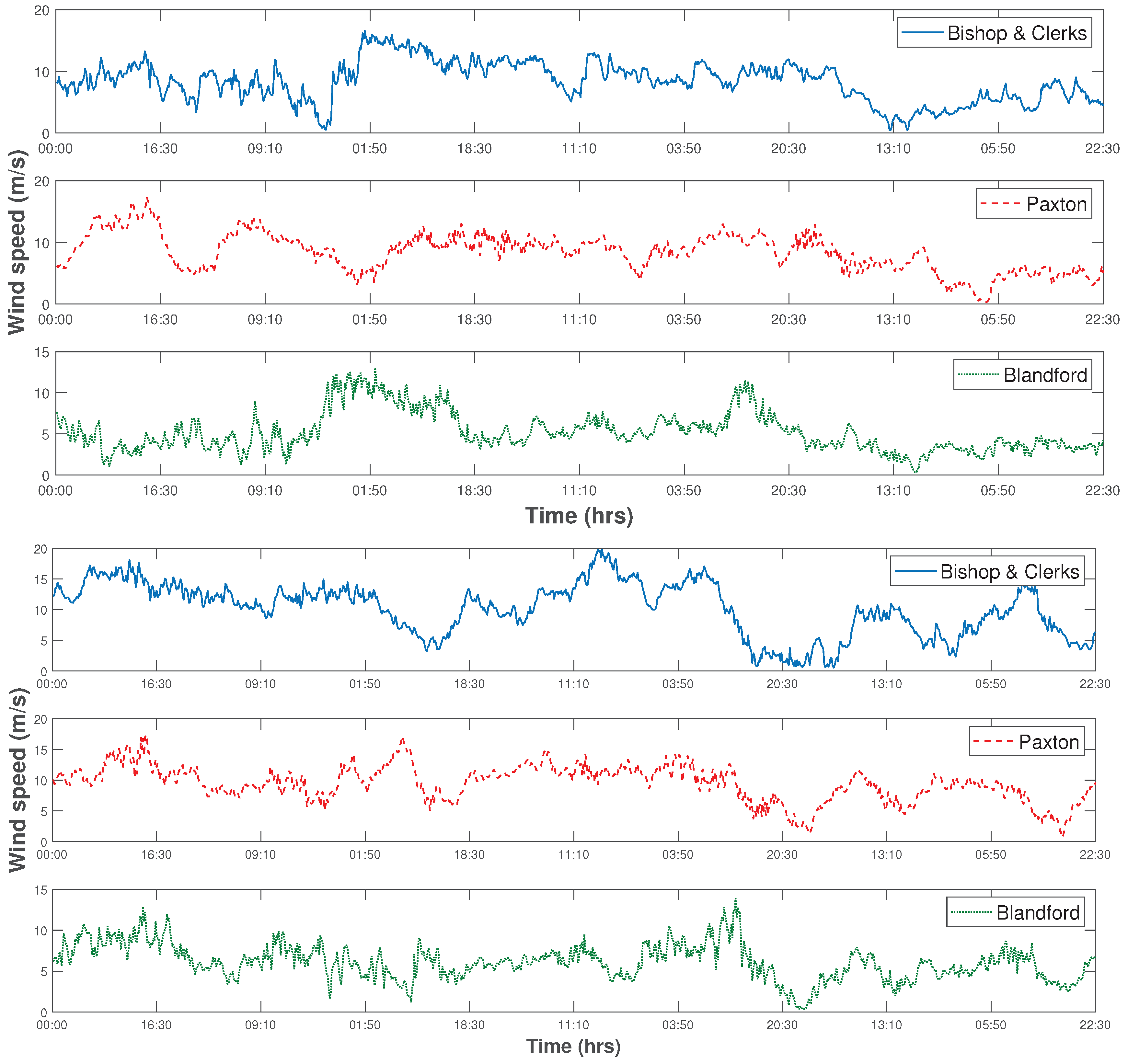
In this section, we implement the MCDM methods for the hybrid operation of wind farms. The wind farms in Massachusetts, namely Bishop & Clerks (Farm A), Paxton (Farm B), and Blandford (Farm C), were selected. Two wind speed datasets were collected from from Wind Energy Center, University of Massachusetts, MA. The wind speed was measured at hub heights of 15 m, 78 m, and 60 m for Farm A, Farm B, and Farm C, respectively, using a cup anemometer. Further, the wind speed for Farm A and Farm B was transformed to a hub height of 60 m using the logarithmic law [24]. The Datasets were labeled D1 (January 2011) and D2 (January 2013) for the three wind farms [25] with their descriptive statistics depicted in

Table 2. Descriptive statistics for wind speed Datasets D1 and D2.

Statistic	D1 (January 2011)			D2 (January 2013)
	Farm A	Farm B	Farm C	Farm A	Farm B	Farm C
Mean	8.3364	8.3612	5.189	10.146	9.4411	6.1096
Std. Dev.	3.2224	3.0543	2.4075	4.2897	2.8944	2.1752
Skewness	−0.0943	−0.1040	0.9670	−0.3428	−0.3219	0.2102

. In the present work, we assumed wind direction facing directly to the turbines, and all the turbines in three wind farms had same rotor diameter of 77 m.

Figure 2 shows the schematic representation for three wind farms along with BESS. The wind farms feed electrical power to a utility grid. In order to approach the MCDM problem, we first evaluated the penalty cost for a particular wind farm (here Bishop & Clerks). The penalty cost was calculated by forecasting the wind power and then comparing it with the actual one. The deficit or surplus wind power windows were then assessed for penalty cost estimation for all four alternatives as discussed in Section 2. The wind speed time series for two datasets at a hub height of 60 m is illustrated in Figure 3. In order to choose the best alternative, we determined the tangible effect of criteria by calculating the penalty cost incurred in all four alternatives. Further, the non-tangible effect was determined by examining the Priority Scores (PS) from MCDM methods. The overall decision was based on cumulative priority score obtained by multiplying the normalized cost score and priority scores.

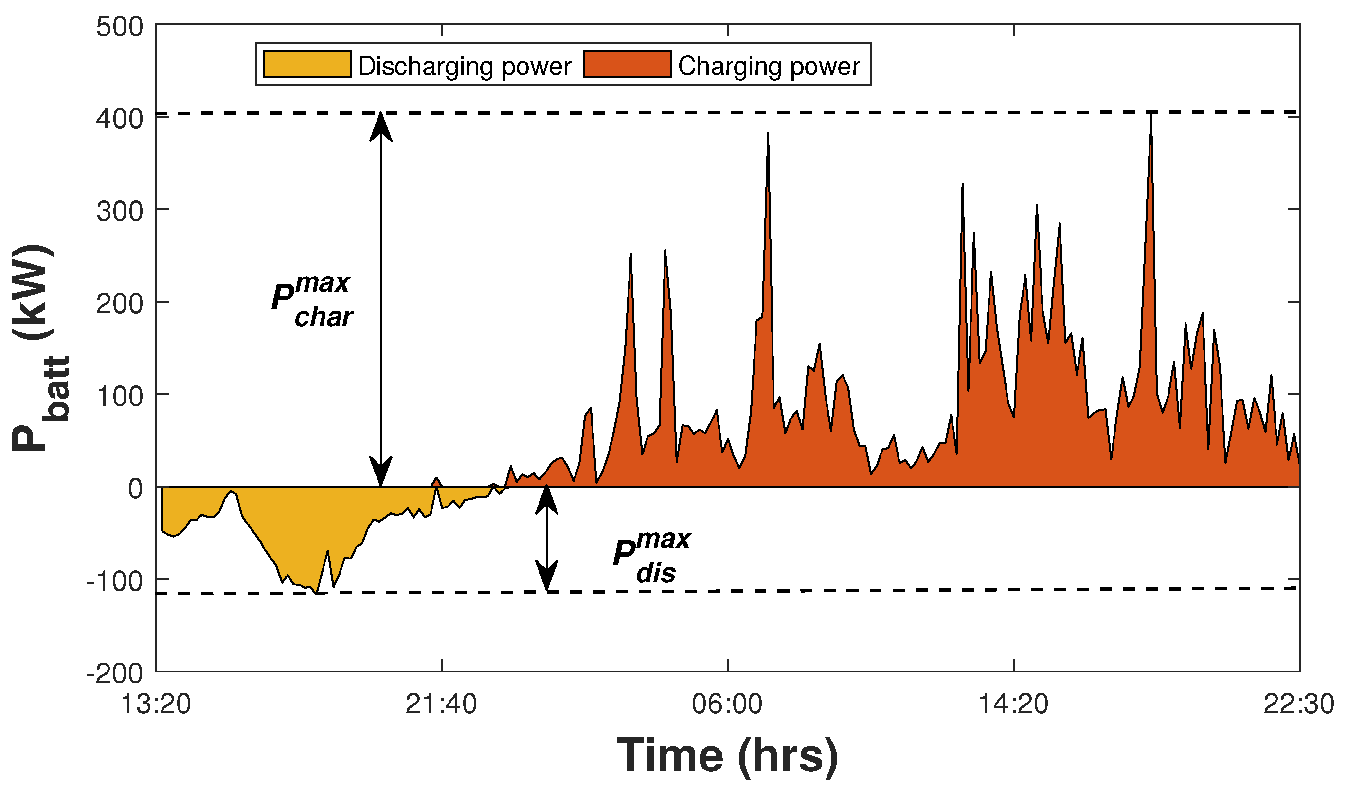
For calculating the penalty cost for the four alternatives, we first forecast the wind speed using Least Squares Support Vector Regression (LSSVR). The dataset of 1000 instances was divided into 800 (training set) and 200 (testing set). Figure 4 shows the magnitude of charging and discharging powers for the BESS for Dataset D1. The BESS power rating was calculated based on the min-max principle as implemented by Nguyen et al., where the cumulative sum of discharging and charging powers was calculated [26].

Table 3. BESS rating for two datasets.

Dataset	BESS Rating	BESS Threshold Limit
$D_1$	15 MW	110 kW
$D_2$	50 MW	955 kW

enlists the BESS power capacity and threshold limit for two datasets D1 and D2.

In the first alternative, the penalty was paid for every 1 kW of incorrect power predicted. Similarly, the penalty cost can be estimated for each alternative ($A_1,A_2,A_3,A_4$). The cost for compensating 1 kW of deficit power in each alternative was $\beta =\$0.5$, $\zeta =\$0.75$, $\alpha =\$0.4$, and $\delta =\$0.8$. The cost of dispatching every 1 kW of incorrect forecasted power using the battery in the case of $A_4$ was chosen as the highest owing to frequent charging and discharging. Further, for calculating cost incurred in alternative $A_2$, the BESS threshold limit was chosen as 110 kW and 955 kW for Datasets D1 and D2, respectively.

Table 4. Penalty cost and normalized cost score for Datasets D1 and D2. PC, Penalty Cost; NCS, Normalized Cost Score.

Alternatives	D1		D2
	PC ($)	NCS	PC ($)	NCS
$A_1$	1971.2	1.1665	6514.2	1.3238
$A_2$	1689.8	1.0000	4920.8	1.0000
$A_3$	3916.5	2.3177	13587	2.7612
$A_4$	2252.8	1.3332	7444.8	1.5129

highlights the Penalty Cost (PC) (in $) and the normalized cost score for each alternative for two datasets D1 and D2.

The Normalized Cost Score (NCS) was calculated by using the minimum normalization technique, that is the minimum cost was assigned a score of one. It must be noted that here, we have determined the normalized cost score considering the tangible effect of penalty cost on decision making. Similarly, the non-tangible effect of criteria on the best alternative was determined by calculating the rank by the conventional MCDM methods. Finally, the rank for the alternatives was determined by calculating the Cumulative Priority Score (CPS), which is arithmetic multiplication of NCS and Priority Score (PS).

Next, we proceeded towards constructing the decision matrix. We had four alternatives ($A_1,A_2,A_3,A_4$) and three criteria ($C_1,C_2,C_3$), as listed in Table 1. The decision matrix elements were based on a semantic relationship between each alternative and criteria, as in

Table 5. Performance scores for the decision matrix [27].

Importance	Performance Score as per AHP	Performance Score in Current Work
Equally Preferred (EP)	1	9
Equally to Moderately Preferred (EMP)	2	8
Moderately Preferred (MP)	3	7
Moderately to Strongly Preferred (MSP)	4	6
Strongly Preferred (SP)	5	5
Strongly to Very strongly Preferred (SVP)	6	4
Very strongly Preferred (VP)	7	3
Very strongly to Extremely Preferred (VEP)	8	2
Extremely Preferred (XP)	9	1

. However, all the criteria in our case were non-beneficial, and so, we used a semantic scale that assigned the highest performance score, that is nine, to the equally-preferred alternative and the lowest score, that is one, to the highly-preferred alternative. In the case of wind wakes, the most preferred alternative was to pay a penalty for power loss due to wakes via batteries, up to a certain threshold, rather than paying for every forecast error. Meanwhile wind curtailment is best dealt with if the curtailed power is fed from batteries. In the case of forced outages, the best alternative was to take a power loan from neighboring farms or to supply power from batteries. However, the latter seems to be more expensive.

In the case of wind wakes, alternative $A_1$ was assigned a score of eight owing to a higher penalty cost incurred to the market operator. Similarly, a score of three and two was assigned to alternatives $A_2$ and $A_3$, respectively, due to lower penalty costs, while $A_4$ was assigned a score of nine due to a higher cost of discharging BESS and thus impacting battery lifetime. For wind curtailment, a score of five and four was assigned to alternatives $A_1$ and $A_2$, respectively, owing to the large penalty paid due to derating of wind turbines, while a score of three was assigned to $A_3$ owing to a lesser penalty cost per kW of deficit wind power forecasted. Forced outage leads to reduction in wind farm capacity, thus choosing alternative $A_1$ would result in paying a higher penalty cost; whereas borrowing wind power from a neighboring farm for lost power due to forced outage will be an economic choice for the farm operator owing to the lesser penalty cost per kW of deficit power. The decision matrix is given as H as per the performance scores stated by Saaty and $H^{\prime }$ as per the our MCDM problem, which assigns the least score to the most preferred alternative.

$$H=\begin{array}{cc}\begin{array}{ccc}{C}_1& C_2& C_3\end{array}& \\ \left(\begin{array}{ccc}2 & 3 & 1\\ 7 & 6 & 4\\ 8 & 7 & 9 \\ 1 & 3 & 2\end{array}\right)& \begin{array}{c}{A}_1\\ A_2\\ A_3\\ A_4\end{array}\end{array}\hspace{1em}{H}^{\prime }=\begin{array}{cc}\begin{array}{ccc}{C}_1& C_2& C_3\end{array}& \\ \left(\begin{array}{ccc}8 & 5 & 9\\ 3 & 4 & 6\\ 2 & 3 & 1\\ 9 & 7 & 8\end{array}\right)& \begin{array}{c}{A}_1\\ A_2\\ A_3\\ A_4\end{array}\end{array}$$

Based on the decision matrix $H^{\prime }$, we then determined the normalized decision matrix using Equation (6) and then the weights for each criteria were obtained as discussed in Section 3.1. The normalized decision matrix for the SAW method is given as:

$$\begin{array}{ccc}\hfill \widehat{H}& =& \left[\begin{array}{ccc}0.2500& 0.6000& 0.1111\\ 0.6667& 0.7500& 0.1667\\ 1.0000& 1.0000& 1.0000\\ 0.2222& 0.4286& 0.1250\end{array}\right]\hfill \end{array}$$

(22)

The weights for the criteria are determined using Equations (8)–(10) and are given as:

$$w=\{0.2864,0.3296,0.3840\}$$

(23)

Based on the weights and normalized matrix, we then calculated the Priority Score (PS) and Cumulative Priority Score (CPS) for the alternatives, which are listed in

Table 6. Ranking using the Simple Additive Weighting (SAW) method.

Alternatives	D1		D2		Ranking
	PS	CPS	PS	CPS
$A_1$	0.3120	0.3640	0.3120	0.4130	3
$A_2$	0.5021	0.5021	0.5021	0.5021	2
$A_3$	1.0000	2.3177	1.0000	2.7612	1
$A_4$	0.2529	0.3372	0.2529	0.3826	4

.

Thus, according to the SAW method, the alternatives were ranked as $A_3\succ A_2\succ A_1\succ A_4$. The best alternative was to pay a penalty for deficit power borrowed from a neighboring wind farm.

Next, we solved the MCDM problem using the COPRAS method. The decision matrix remained the same for all the methods. However, while normalizing the decision matrix, we used Equation (12). The normalized decision matrix is given as:

$$\begin{array}{ccc}\hfill \widehat{H}& =& \left[\begin{array}{ccc}0.6364& 0.5025& 0.6671\\ 0.2387& 0.4020& 0.4447\\ 0.1591& 0.3015& 0.0741\\ 0.7160& 0.7035& 0.5930\end{array}\right].\hfill \end{array}$$

(24)

Meanwhile the weights were calculated using the entropy method stated in (Section 3.1) and are given as:

$$w=\{0.4142,0.1201,0.4658\}.$$

(25)

Based on the weights and normalized matrix, we then calculated the priority and cumulative priority score for the alternatives using Equations (20) and (21), which are listed in

Table 7. Cumulative priority score and ranking based on the Complex Proportional Assessment (COPRAS) method.

Alternatives	D1		D2		Ranking
	PS	CPS	PS	CPS	D1	D2
$A_1$	0.2153	0.2511	0.2153	0.2850	4	4
$A_2$	0.3857	0.3857	0.3857	0.3857	2	2
$A_3$	1.0000	2.3177	1.0000	2.7612	1	1
$A_4$	0.2079	0.2772	0.2079	0.3145	3	3

.

Thus, according to the COPRAS method, the alternatives were ranked as $A_3\succ A_2\succ A_4\succ A_1$. The best alternative was to pay a penalty for taking a power loan from a neighboring wind farm. However, this choice seems far fetched due to uncertainties in the neighboring wind farm(s).

Finally, we solved the MCDM problem using the TOPSIS method for which the normalized decision matrix was obtained using Equation (12), and weights were calculated using the entropy method. The normalized matrix and weights are given as:

$$\begin{array}{ccc}\hfill \widehat{H}& =& \left[\begin{array}{ccc}0.6364& 0.5025& 0.6671\\ 0.2387& 0.4020& 0.4447\\ 0.1591& 0.3015& 0.0741\\ 0.7160& 0.7035& 0.5930\end{array}\right].\hfill \end{array}$$

(26)

Meanwhile the weights were calculated using entropy method stated in Section 3.1 and are given as:

$$w=\{0.4142,0.1201,0.4658\}.$$

(27)

Next, we identified positive and negative ideal solutions using Equations (14) and (15), given as:

$$\begin{array}{cc}\hfill S^{+}& =\{0.0659,0.0362,0.0345\},\end{array}$$

(28)

$$\begin{array}{cc}\hfill S^{-}& =\{0.2965,0.0845,0.3107\}.\end{array}$$

(29)

Further, the Euclidean distance from the positive ideal and negative ideal solutions was calculated using Equations (16) and (17), where $p=2$ and is found as:

$$\begin{array}{ccc}\hfill D^{+}& =& \{0.0580,0.0155,0,0.0570\}, \hfill \end{array}$$

(30)

$$\begin{array}{ccc}\hfill D^{-}& =& \{0.0008,0.0256,0.0659,0.0006\}.\hfill \end{array}$$

(31)

Finally, the relative priority and cumulative priority score was calculated for all the alternatives, which are ranked in

Table 8. Ranking using the TOPSIS method.

Alternatives	D1		D2		Ranking
	PS	CPS	PS	CPS
$A_1$	0.0142	0.0166	0.0142	0.0188	3
$A_2$	0.5323	0.5323	0.5323	0.5323	2
$A_3$	1.0000	2.3177	1.0000	2.7612	1
$A_4$	0.0104	0.0139	0.0104	0.0157	4

.

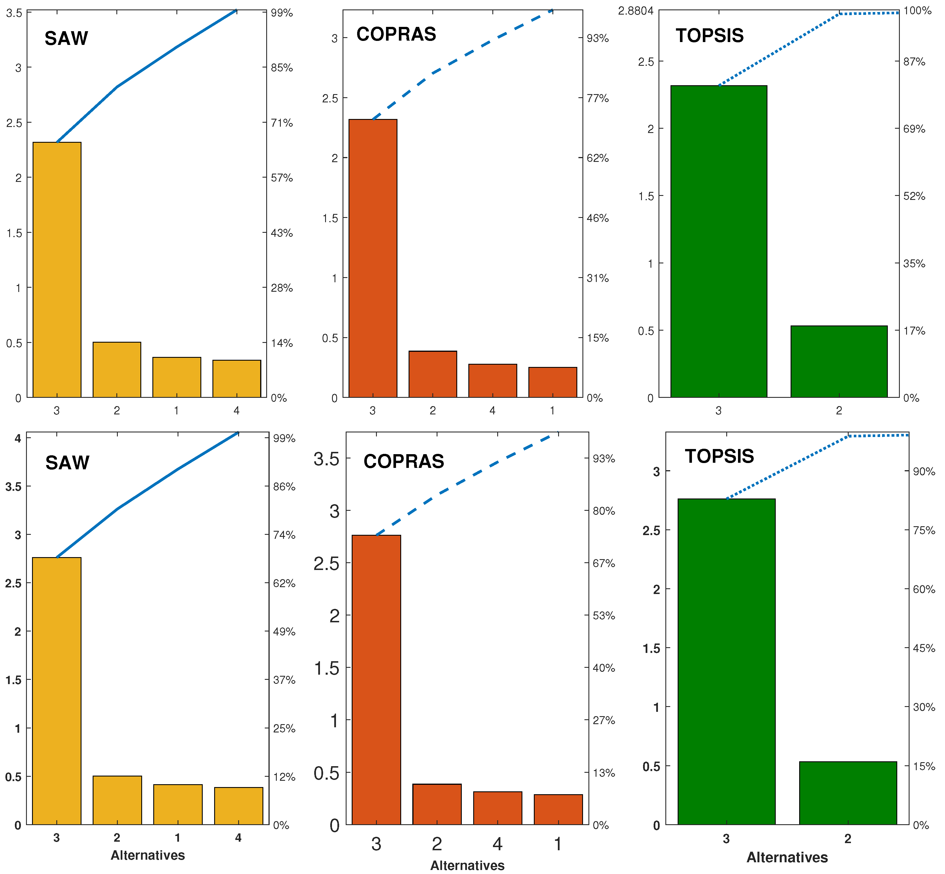
Thus, according to the TOPSIS method, the alternatives were ranked as $A_3\succ A_2\succ A_1\succ A_4$. The best alternative was to pay a penalty for deficit power borrowed from a neighboring wind farm. The MCDM methods carried out for hybrid operation of wind farms revealed paying a penalty for borrowed power from a neighboring wind farm as the best alternative. The results of all three methods were validated based on tangible and non-tangible effects from all the criteria. The ranking and priority scores for all the alternatives along with their priority score as illustrated in the form of a Pareto chart graph are shown in Figure 5.

5. Comparative Analysis of MCDM Methods

It is well accepted that identifying the most appropriate MCDM approach from the list of existing several methods for a given application is a difficult task. This is due to the inherent benefits and limitations possessed by each of the methods. This paper pioneered a methodology to evaluate different MCDM methods in the wind farm application domain based on the data requirement and the effects of dynamic decision matrices and rank reversal.

The number of data D required in the decision process: This parameter evaluates the number of data required from the DMs for adopting the considered MCDM methods to evaluate optimized hybrid wind power generation techniques. Let i be the number of hybrid wind power generation strategies and j be the number of assessment criteria; therefore, the required number of data required D in each of the considered MCDM methods for the decision matrix is given as:

$$D=(i+1)j.$$

(32)

For the presented case study, all three considered methods, that is SAW, TOPSIS, and COPRAS, required only 15 judgments. Therefore, it can be stated that all three methods performed similarly in terms of the level of communication with the DMs for data collection.

In spite of having the considerable significance of MCDM methods in framing efficient assessment models, there are many criticisms of these methods due to the occurrence of Rank Reversal (RR). RR mostly refers to a change in the ranking of a preferred alternative when some other alternative is added or removed in the original decision matrix. In real-life situations, a concerned problem may amend or change from time to time while taking into account the changes in existing decision matrices due to the introduction or removal of a new alternative. When the hybrid wind power generation strategy selection problem was solved by the SAW method, the ranking was generated as $A_3\succ A_2\succ A_1\succ A_4$, as given in Table 6, which clearly indicates strategy $A4$ as the worst option. Now, due to its poor performance and rank, strategy $A_4$ was dropped from the alternative list, and the new decision matrix (consisting of three alternatives) or the dynamic decision matrix was again solved using the SAW, TOPSIS, and COPRAS methods. The new ranking as given by these three methods with the same criteria weights was $A_3\succ A_2\succ A_1$, indicating $A_3$ still as the best alternative and $A_1$ as the worst alternative, as shown in Table 8. From this table, it is clear that when alternative $A_4$ was deleted, there was no change in the ranking of the other three alternative strategies. Further proceeding towards deletion of all the worst alternatives from the subsequent dynamic decision matrices, it has been observed that there was no effect of the dynamic decision matrices on any of the three methods. $A_3$ remained the best strategy for all the considered alternations in the decision matrices, thus establishing the robustness and accuracy of these methods for ranking alternatives under a dynamic environment as depicted in

Table 9. Ranking under dynamic decision matrices in the SAW, TOPSIS, and COPRAS methods.

Alternatives	Initial	A4	A1	A2
	Rank
$A_4$	4
$A_1$	3	3
$A_2$	2	2	2
$A_3$	1	1	1	1

.

Based on the above analyses, it can be concluded that the adopted methods are very credible, which can be successfully used for rational decision making.

6. Conclusions

A multi-criteria decision making problem for the economic operation of a wind farm was presented with a set of four alternatives, which were assessed for three criteria. Wind wakes, wind curtailment and forced outage govern the optimal strategy for a wind operator. The decision matrix was created based on our understanding and judgment of each criterion on a particular alternative. The cumulative priority scores were calculated for three MCDM methods. The hybrid operation of the wind farm was characterized by four alternatives based on three criteria evaluated based on three MCDM methods. For SAW and TOPSIS, we obtained the ranking as $A_3\succ A_2\succ A_1\succ A_4$, whereas for COPRAS, $A_3\succ A_2\succ A_4\succ A_1$. The rank reversal in this case was tested by removing $A_4$ and $A_1$, and the results revealed $A_3$ as the best preferred choice. Given an accurate forecasting scheme, paying a penalty cost for borrowed deficit power from a neighboring wind farm will result in the economic operation of the wind farm. Further, the current MCDM problem can be extended considering the uncertainties in individual wind farms like in the case of wind wakes by implementing the fuzzy TOPSIS method.

References

- Abhinav, R.; Pindoriya, N.M. Opportunities and key challenges for wind energy trading with high penetration in Indian power market. Energy Sustain. Dev. 2018, 47, 53–61. [Google Scholar] [CrossRef]
- Hur, S.-H. Modelling and control of a wind turbine and farm. Energy 2018, 156, 360–370. [Google Scholar] [CrossRef]
- Majumder, M. Impact of Urbanization on Water Shortage in Face of Climatic Aberrations; Springer: Singapore, 2015. [Google Scholar]
- Keyser, W.D.; Peeters, P. A note on the use of PROMETHEE multicriteria methods. Eur. J. Oper. Res. 1996, 89, 457–461. [Google Scholar] [CrossRef]
- Haralambopoulos, D.; Polatidis, H. Renewable energy projects: Structuring a multi-criteria group decision making framework. Renew. Energy 2003, 28, 961–973. [Google Scholar] [CrossRef]
- Georgiou, D.; Mohammed, E.S.; Rozakis, S. Multi-criteria decision making on the energy supply configuration of autonomous desalination units. Renew. Energy 2015, 75, 459–467. [Google Scholar] [CrossRef]
- Kundakcı, N. An integrated method using MACBETH and EDAS methods for evaluating steam boiler alternatives. J. Multi-Criteria Decis. Anal. 2018, 26, 27–34. [Google Scholar] [CrossRef]
- Lee, A.H.; Hung, M.C.; Kang, H.Y.; Pearn, W. A wind turbine evaluation model under a multi-criteria decision making environment. Energy Convers. Manag. 2012, 64, 289–300. [Google Scholar] [CrossRef]
- Mahdy, M.; Bahaj, A.S. Multi criteria decision analysis for offshore wind energy potential in Egypt. Renew. Energy 2018, 118, 278–289. [Google Scholar] [CrossRef] [Green Version]
- Kolios, A.; Rodriguez-Tsouroukdissian, A.; Salonitis, K. Multi-criteria decision analysis of offshore wind turbines support structures under stochastic inputs. Ships Offshore Struct. 2016, 11, 38–49. [Google Scholar]
- Garni, H.A.; Kassem, A.; Awasthi, A.; Komljenovic, D.; Al-Haddad, K. A multicriteria decision making approach for evaluating renewable power generation sources in Saudi Arabia. Sustain. Energy Technol. Assess. 2016, 16, 137–150. [Google Scholar] [CrossRef]
- Jahan, A.; Edwards, K.L. A state-of-the-art survey on the influence of normalization techniques in ranking: Improving the materials selection process in engineering design. Mater. Des. (1980–2015) 2015, 65, 335–342. [Google Scholar] [CrossRef]
- Deng, Y.; Yu, Z.; Liu, S. A review on scale and siting of wind farms in China. Wind Energy 2010, 14, 463–470. [Google Scholar] [CrossRef] [Green Version]
- Patel, P.; Shandilya, A.; Deb, D. Optimized hybrid wind power generation with forecasting algorithms and battery life considerations. In Proceedings of the 2017 IEEE Power and Energy Conference at Illinois (PECI), Champaign, IL, USA, 23–24 February 2017. [Google Scholar]
- Henriot, A. Economic curtailment of intermittent renewable energy sources. Energy Econ. 2015, 49, 370–379. [Google Scholar] [CrossRef]
- Roth, M. Renewable Energy and Landscape Quality; Jovis Verlag: Berlin, Germany, 2018. [Google Scholar]
- Lowson, M.V. Assessment and Prediction of Wind Turbine Noise; Technical report; Flow Solutions Ltd.: Bristol, UK, 1993; ETSU-W–13/00284/REP. [Google Scholar]
- Hwang, C.L.; Yoon, K. Methods for Multiple Attribute Decision Making. In Multiple Attribute Decision Making: Methods and Applications A State-of-the-Art Survey; Springer: Berlin/Heidelberg, Germany, 1981; pp. 58–191. [Google Scholar] [CrossRef]
- Byun, H.; Lee, K. A decision support system for the selection of a rapid prototyping process using the modified TOPSIS method. Int. J. Adv. Manuf. Technol. 2005, 26, 1338–1347. [Google Scholar] [CrossRef]
- Lourenzutti, R.; Krohling, R.A. A generalized TOPSIS method for group decision making with heterogeneous information in a dynamic environment. Inf. Sci. 2016, 330, 1–18. [Google Scholar] [CrossRef]
- Balioti, V.; Tzimopoulos, C.; Evangelides, C. Multi-Criteria Decision Making Using TOPSIS Method Under Fuzzy Environment. Application in Spillway Selection. Proceedings 2018, 2, 637. [Google Scholar] [CrossRef]
- Zolfani, S.H.; Chen, I.S.; Rezaeiniya, N.; Tamošaitienė, J. A hybrid mcdm model encompassing AHP and COPRAS-G methods for selecting company supplier in iran. Technol. Econ. Dev. Econ. 2012, 18, 529–543. [Google Scholar] [CrossRef]
- Bhowmik, C.; Bhowmik, S.; Ray, A. The effect of normalization tools on green energy sources selection using multi-criteria decision making approach: A case study in India. J. Renew. Sustain. Energy 2018, 10, 065901. [Google Scholar] [CrossRef]
- Tennekes, H. The Logarithmic Wind Profile. J. Atmos. Sci. 1973, 30, 234–238. [Google Scholar] [CrossRef] [Green Version]
- Bishop and Clerks, Nantucket Sound|Wind Energy Center. Available online: https://www.umass.edu/windenergy/resourcedata/Bishop_and_Clerks (accessed on 20 February 2019).
- Nguyen, C.L.; Lee, H.H.; Chun, T.W. Cost-Optimized Battery Capacity and Short-Term Power Dispatch Control for Wind Farm. IEEE Trans. Ind. Appl. 2015, 51, 595–606. [Google Scholar] [CrossRef]
- Saaty, R. The analytic hierarchy process—what it is and how it is used. Math. Model. 1987, 9, 161–176. [Google Scholar] [CrossRef] [Green Version]
Figure 1.
Schematic representation of the multi-criteria decision making problem for wind farms.
Figure 2.
Schematic diagram for three wind farms in Massachusetts.
Figure 3.
Wind speed pattern for three wind farms in Massachusetts.
Figure 4.
BESS charging and discharging power for Bishop & Clerks, January 2011.
Figure 5.
Pareto charts for alternatives for Datasets D1 and D2.