Some Normal Intuitionistic Fuzzy Heronian Mean Operators Using Hamacher Operation and Their Application

Abstract

Hamacher operation is a generalization of the algebraic and Einstein operation and expresses a family of binary operation in the unit interval [0,1]. Heronian mean can deal with correlations of different criteria or input arguments and does not bring out repeated calculation. The normal intuitionistic fuzzy numbers (NIFNs) can depict normal distribution information in practical decision making. A decision-making problem was researched under the NIFN environment in this study, and a new multi-criteria group decision-making (MCGDM) approach is herein introduced on the basis of Hamacher operation. Firstly, according to Hamacher operation, some operational laws of NIFNs are presented. Secondly, it is noted that Heronian mean not only takes into account mutuality between the attribute values once, but also considers the correlation between input argument and itself. Therefore, in order to aggregate NIFN information, we developed some operators and studied their properties. These operators include Hamacher Heronian mean (NIFHHM), Hamacher weighted Heronian mean (NIFHWHM), Hamacher geometric Heronian mean (NIFHGHM), and Hamacher weighted geometric Heronian mean (NIFHWGHM). Furthermore, we applied the proposed operators to the MCGDM problem and developed a new MCGDM approach. The characteristics of this new approach are that: (1) it is suitable for making a decision under the NIFN environment and it is more reasonable for aggregating the normal distribution data; (2) it utilizes Hamacher operation to provide an effective and powerful MCGDM algorithm and to make more reliable and more flexible decisions under the NIFN circumstance; (3) it uses the Heronian mean operator to deal with interrelations between the attributes or input arguments, and it does not bring about repeated calculation. Therefore, the proposed method can describe the interaction of the different criteria or input arguments and offer some reasonable and reliable MCGDM aggregation operators, which can open avenues for decision making and broaden perspectives of the decision experts. Lastly, an application is given for showing the effectiveness and feasibility of the approach presented in this paper.

1. Introduction

In the MCGDM procedure, because a lot of problems are uncertain or fuzzy, the value of the input argument is not always a real number and may be more effectively described as a fuzzy value. Zadeh’s fuzzy set (FS) plays an important role in dealing with fuzzy number information [1], and the FS theory has been a good tool which is suitable for various fields, including decision analysis, machine learning, information retrieval, among others.

However, the FS theory only defines a membership function in a domain of discourse, so it is very difficult to describe the vagueness and uncertainty of the objective elements in real society [2]. The intuitionistic fuzzy set (denoted as IFS) theory [3] involves a non-membership function besides a membership function. Recently, the IFS theory has been applied to the MCGDM field. Xu presented some aggregation methods under an intuitionistic fuzzy number circumstance to settle MCGDM problems [4,5]. The IFS was generalized to the interval-valued IFS (denoted as IVIFS) by Gargov [6] and Atanassov [7]. Xu and Yager [8] proposed a new measurement method similar to the IVIFSs for dealing with the MCGDM problem. Tan and Zhang [9] gave a new TOPSIS approach which can deal with a decision-making problem with interval-valued intuitionistic fuzzy number (IVIFN) data. Wang et al. [10] utilized the prospect value function to introduce a score method which can settle the MCGDM problem under the IVIFN environment. Gomathi Nayagam et al. [11] defined an accuracy function of the IVIFNs. Fuzzy number IFS (denoted as FNIFS) theory was proposed by Liu and Yuan [12], where some basic operational laws were defined and the relationships among the FNIFS, the IFS, and interval-valued fuzzy set (IVFS) were discussed. Shu et al. [13] introduced the triangular IFNs (TriIFNs) and presented the operational rules which are utilized in fault-tree analysis. Lin et al. [14] proposed some prioritized operators for the FNIF data. Furthermore, they presented a method to deal with fuzzy number intuitionistic fuzzy MCGDM problems. Wang [15] extended the TriIFNs and originally defined the TriIFNs and IVTriIFNs. The trapezoidal intuitionistic fuzzy numbers (TraIFNs) [16,17,18,19,20,21] are other types of the IFNs. Some MCGDM processes were studied for the TriIFNs or TraIFNs information [22,23,24,25,26,27,28,29,30].

In nature, a lot of social and economic phenomena involve some normal distribution factors, such as random measurement error, average annual rainfall in a region, and others. Yang and Ko [31] proposed the concept with respect to the normal fuzzy numbers (NFNs), which are very suitable for depicting normal distribution information. Wang et al. [32,33] gave the definition of the normal intuitionistic (NIFNs), and they introduced some operations and score function of the NIFNs. Some MCGDM problems were discussed in order to deal with NIFN information [34,35], and some new operators were developed. Nevertheless, these aggregation operators only focus on the impact of input data and ordered result, and they cannot present the interrelationship of input data. Some normal intuitionistic fuzzy Bonferroni mean operators were proposed by Liu and Liu [36] for describing the correlation of input data. Bonferroni originally proposed the Bonferroni mean (BM) in 1950, which considers mutuality of attribute values [37,38]. The BM operators were studied in regard to the circumstance under which the criterion values may be other types, such as NIFNs, HFNs [39], IFNs [40], IVIFNs [41], and IVNs [42].

Heronian mean (denoted as HM) [43,44,45] is another type of decision-making operator which can also objectively express the interrelations between input data. The significant characteristics of the HM operator are that (1) it can account for the interaction of the different criteria or input arguments, which is very desirable in decision making; (2) it pays close attention to the aggregated input data, and it is not the same as power operator or integral aggregation operator, which focus on the importance of the attributes or input data; (3) it can capture the interrelation between an attribute and itself, and take into account the correlation between an input argument and itself. From the definition of the BM and HM operators, the BM operator indicates the correlation between the criteria $c_i$ and $c_j$ ($i\ne j$). However, the correlation between $c_i$ and $c_j$ is equal to the correlation between $c_j$ and $c_i$ ($i\ne j$). Namely, the BM operator results in the redundant computation. Furthermore, it ignores the correlation between criterion $c_i$ and itself. Although the HM decision operator is similar to the BM aggregation operator, it can settle the aforementioned shortcoming of the BM aggregation operator. At present, the HM has been applied to aggregate the input information with the IFNs [46], the hesitant fuzzy set (HFS) information [47] and the IVIFN [48].

However, the HM is not applied to aggregate the normal intuitionistic fuzzy number (NIFN) arguments. The above aggregation operators only take into account the algebraic operation of the IFNs, hesitant fuzzy set (HFS), IVIFNs, or NIFNs where the algebraic product and sum are important, and they can define union and intersection of the NIFNs, IVIFNs, or HFS. In conclusion, a generalized t-conorm or t-norm can simulate union and intersection between the IFNs or IVIFNs [49,50]. According to Archimedean t-conorm or t-norm, Xia et al. [50] generalized the Hamacher and Frank operational laws and presented some operational laws of the IFNs. Furthermore, they introduced the weighted average and geometric operator for the intuitionistic fuzzy MCGDM problem. Because these operators do not integrate the weight of the attribute and order, they cannot be utilized for IVIFNs. Wang and Liu [51,52] applied the Einstein operation to develop some operators.

Hamacher operation generalizes the algebraic and Einstein operation, and it also plays an important role in studying aggregation method for the MCGDM problem [53]. Hamacher operation depends on Hamacher t-norm and Hamacher t-conorm, which are a pair of dual triangular norms. In other words, Hamacher t-norm or Hamacher t-conorm are binary operations in the unit interval [0,1] which satisfy boundary, monotonicity, associativity, and symmetry, and they are broadly applicable in the FS theory, fuzzy logic, and information aggregation. Especially, as for any hot research topic, Hamacher operation has been applied to aggregate the IFN information, IVIFN information [54], or hesitant fuzzy information.

First of all, in the practical MCGDM procedure, there are many natural phenomena which approximately obey normal distribution. Furthermore, the criteria or input arguments are often stochastic values or fuzzy values, and sometimes the stochastic and fuzzy values exist simultaneously. Under these special circumstances, the IFNs cannot accurately express random information. As an expansion of the IFNs and NFNs, the NIFNs can better describe fuzzy MCGDM problems with normal distribution. Besides this, in the MCGDM process, there is an interaction among the different criteria or input arguments, especially, and some unreasonable information values are determined by the decision maker. Therefore, it is very important to determine how to depict simultaneously stochastic and fuzzy information and how to capture the interaction of the different criteria or input arguments in order to make a reasonable decision by more general and more flexible MCGDM approach.

According to the aforementioned analysis, we note that there are no methods aggregating NIFNs with respect to Hamacher operation and considering the interrelationship between NIFN arguments at the same time. The NIFNs can simultaneously describe the fuzzy and random information, and the HM operator can better capture and handle the correlation between the different criteria or input data and relieve the redundant computation at the same time. Hamacher operation can offer more flexible operation or more general operation for a reasonable MCGDM procedure. Therefore, in this paper, the motivation of the research is (1) to present some new operational laws of the NIFNs on the basis of the Hamacher t-norm and Hamacher t-conorm; (2) to propose some new HM operators and study some of their desirable properties; (3) to develop a new MCGDM approach which can deal with the NIFNs information.

This paper is presented as follows. In Section 2, we review the normal intuitionistic fuzzy number, Hamacher operation, and Heronian mean operators. In Section 3, we establish Hamacher operational rules and their characteristics with respect to the normal intuitionistic fuzzy numbers, furthermore, we describe the normal intuitionistic fuzzy Heronian mean aggregation operators based on Hamacher operation of NIFNs and study their properties. According to the new Hamacher operations, the geometric Heronian mean is extended to the NIFNs, and its weighted version is presented in Section 4. In Section 5, we utilize new operators to make a MCGDM procedure for the NIFN information and introduce the decision steps. In Section 6, an application is introduced to show the new approach and the evidence of the effectiveness. We make a conclusion and present some remarks in Section 7.

2. Preliminaries

Some notions and operational rules with respect to NIFNs are introduced in this section, and the definition of Heronian mean operator is given.

2.1. Normal Intuitionistic Fuzzy Number

Definition 1.

[31] If$R$is a real number set, and$x,\alpha ,\sigma \in R$,$A=\left(\alpha ,\sigma \right)$is a normal fuzzy number (NFN) whose membership function is presented

$$A\left(x\right)=e^{-{\left(\frac{x-a}{\sigma }\right)}^2},\sigma >0$$

(1)

Definition 2.

[33] If$X$is a finite nonempty set, a normal intuitionistic fuzzy number (NIFN)$A=\langle \left(\alpha ,\sigma \right),{\mu }_A,v_A\rangle$is presented in the following, where${\mu }_A$is the membership function and$v_A$is the non-membership function, and they satisfy$0\le {\mu }_A\le 1$,$0\le v_A\le 1$,$0\le {\mu }_A+v_{A}v\le 1$.

$${\mu }_A\left(x\right)={\mu }_A{e}^{-{\left(\frac{x-\alpha }{\sigma }\right)}^2},x\in X$$

(2)

$$v_A\left(x\right)=1-\left(1-v_A\right)e^{-{\left(\frac{x-\alpha }{\sigma }\right)}^2},x\in X$$

(3)

Compared with the classical IFNs, the non-membership function of the NIFNs can more synthetically capture the fuzziness and uncertainty of objects. From the definition of NIFNs, its universe of discourse is expanded from discrete to continuous, and it can effectively describe a large number of normal distributions under the socioeconomic environment. In the following, some operational rules of the NIFNs were defined in [33].

Let $A_i=\langle \left({\alpha }_i,{\sigma }_i\right),{\mu }_i,v_i\rangle ,i=1,2$, and $A=\langle \left(\alpha ,\sigma \right),\mu ,v\rangle$, $\gamma >0,\lambda >0$, then

$$A_1\oplus A_2=\langle \left({\alpha }_1+{\alpha }_2,{\sigma }_1+{\sigma }_2\right),{\mu }_1+{\mu }_2-{\mu }_1{\mu }_2,v_1{v}_2\rangle$$

(4)

$$A_1\otimes A_2=\langle \left({\alpha }_1{\alpha }_2,{\alpha }_1{\alpha }_2\sqrt{\frac{{\sigma }_1^2}{{\alpha }_1^2}+\frac{{\sigma }_2^2}{{\alpha }_2^2}}\right),{\mu }_1{\mu }_2,v_1+v_2-v_1{v}_2\rangle$$

(5)

$$\lambda A=\langle \left(\lambda \alpha ,\lambda \sigma \right),1-{\left(1-\mu \right)}^{\lambda },v^{\lambda }\rangle$$

(6)

$$A^{\lambda }=\langle \left({\alpha }^{\lambda },{\lambda }^{\frac{1}{2}}{\alpha }^{\lambda -1}\sigma \right),{\mu }^{\lambda },1-{\left(1-v\right)}^{\lambda }\rangle$$

(7)

The score and accuracy function with respect to NIFNs are given as follows [33]:

$$S_1\left(A\right)=\alpha \left({\mu }_A-v_A\right),S_2\left(A\right)=\sigma \left({\mu }_A-v_A\right)$$

(8)

$$H_1\left(A\right)=\alpha \left({\mu }_A+v_A\right),H_2\left(A\right)=\sigma \left({\mu }_A+v_A\right)$$

(9)

In order to rank any two NIFNs, the following method was introduced by Wang and Li [33].

If $S_1\left(A_1\right)>S_1\left(A_2\right)$, then $A_1>A_2$;

If $S_1\left(A_1\right)=S_1\left(A_2\right)$, and $H_1\left(A_1\right)>H_1\left(A_2\right)$, then $A_1>A_2$;

If $S_1\left(A_1\right)=S_1\left(A_2\right)$ and $H_1\left(A_1\right)=H_1\left(A_2\right)$, then;

If $S_2\left(A_1\right)<S_2\left(A_2\right)$ then $A_1>A_2$;

If $S_2\left(A_1\right)=S_2\left(A_2\right)$ and $H_2\left(A_1\right)<H_2\left(A_2\right)$ then $A_1>A_2$;

If $S_2\left(A_1\right)=S_2\left(A_2\right)$ and $H_2\left(A_1\right)=H_2\left(A_2\right)$ then $A_1=A_2$.

2.2. Hamacher t-Norm and Hamacher t-Conorm

In FS theory, t-conorm ($T^{*}$) and t-norm ($T$) are very important to the generalization of intersection or union of fuzzy sets [34,42,46,55,56,57,58,59,60,61].

Definition 3.

[46] If$A$and$B$are IFSs, then the union and intersection of$A$and$B$are expressed

$$A{\cup }_{T{T}^{*}}B=\left\{\langle x,T^{*}\left({\mu }_A\left(x\right),{\mu }_B\left(x\right)\right),T\left(v_A\left(x\right),v_B\left(x\right)\right)\rangle ,x\in X\right\}$$

(10)

$$A{\cap }_{T{T}^{*}}B=\left\{\langle x,T\left({\mu }_A\left(x\right),{\mu }_B\left(x\right)\right),T^{*}\left(v_A\left(x\right),v_B\left(x\right)\right)\rangle ,x\in X\right\}$$

(11)

Hamacher defined the Hamacher t-norm and Hamacher t-conorm [10,56]:

$$T_{\gamma }\left(x,y\right)=\frac{xy}{\gamma +\left(1-\gamma \right)\left(x+y-xy\right)},\gamma >0$$

(12)

$$T_{\gamma }^{*}\left(x,y\right)=\frac{x+y-xy-(1-\gamma )xy}{1-(1-\gamma )xy},\gamma >0$$

(13)

Especially, when $\gamma =1$, Hamacher t-norm and Hamacher t-conorm transform into the algebraic t-norm and t-conorm:

$$T\left(x,y\right)=xy,T^{*}\left(x,y\right)=x+y-xy$$

(14)

If $\gamma =2$, Hamacher t-norm and Hamacher t-conorm are respectively equal to the Einstein t-norm and t-conorm [39].

$$T\left(x,y\right)=\frac{xy}{1+\left(1-x\right)\left(1-y\right)}{T}^{*}\left(x,y\right)=\frac{x+y}{1+xy}$$

(15)

2.3. Heronian Mean

Definition 4.

[43] Let$a_i\left(i=1,2,\cdots ,n\right)\in R$, which is greater than zero. The basic Heronian mean (BHM) is defined as follows

$$BHM\left(a_1,a_2,\cdots ,a_n\right)=\frac{2}{n\left(n+1\right)}{\displaystyle \sum _{i=1}^n{\displaystyle \sum _{j=i}^n\sqrt{a_i{a}_j}}}$$

(16)

Based on the BHM, Yu and Wu [48] applied the parameters $p$ and $q$ to the BHM and obtained a more general HM version, and they proposed the geometric Heronian mean.

Definition 5.

[48] Let$p,q>0$and$a_i\in R,a_i\ge 0\left(i=1,2,\cdots ,n\right)$, then the HM aggregation operator is presented in the following

$$H{M}^{p,q}\left(a_1,a_2,\cdots ,a_n\right)={\left(\frac{2}{n\left(n+1\right)}{\displaystyle \sum _{i=1}^n{\displaystyle \sum _{j=i}^n{a}_i^p{a}_j^q}}\right)}^{\frac{1}{p+q}}$$

(17)

It is easy to notice that the HM reduces to the BHM when $p=q=\frac{1}{2}$.

Definition 6.

[48] If$p,q\ge 0$and$p,q$are not equal to zero at the same time,$a_i\in R,a_i\ge 0,i=1,2,\cdots ,n$, then the geometric Heronian mean (denoted as GHM) has the following form

$$GH{M}^{p,q}\left(a_1,a_2,\cdots ,a_n\right)=\frac{1}{p+q}\left({\displaystyle \prod _{i=1,j=i}^n{\left(p{a}_i+q{a}_j\right)}^{\frac{2}{n\left(n+1\right)}}}\right)$$

(18)

3. Normal Intuitionistic Fuzzy Hamacher Heronian Mean Operator and Its Weighted Form

3.1. Hamacher Operational Laws of the NIFNs

From Definition 3—Hamacher t-norm and Hamacher t-conorm—Hamacher intersection and sum between NIFNs are introduced.

Suppose that $A_i=\langle \left({\alpha }_i,{\sigma }_i\right),{\mu }_i,v_i\rangle i=1,2$, $A=\langle \left(\alpha ,\sigma \right),\mu ,v\rangle$, $\gamma >0\lambda \text{>}0$. The Hamacher operational rules of the NIFNs are presented as follows:

$$A_1{\oplus }_H{A}_2=\langle \left({\alpha }_1+{\alpha }_2,{\sigma }_1+{\sigma }_2\right),\frac{{\mu }_1+{\mu }_2-{\mu }_1{\mu }_2-\left(1-\gamma \right){\mu }_1{\mu }_2}{1-\left(1-\gamma \right){\mu }_1{\mu }_2},\frac{v_1{v}_2}{\gamma +\left(1-\gamma \right)\left(v_1+v_2-v_1{v}_2\right)}\rangle$$

(19)

$$A_1{\otimes }_H{A}_2=\langle \left({\alpha }_1{\alpha }_2,{\alpha }_1{\alpha }_2\sqrt{\frac{{\sigma }_1^2}{{\alpha }_1^2}+\frac{{\sigma }_2^2}{{\alpha }_2^2}}\right),\frac{{\mu }_1{\mu }_2}{\gamma +\left(1-\gamma \right)\left({\mu }_1+{\mu }_2-{\mu }_1{\mu }_2\right)},\frac{v_1+v_2-v_1{v}_2-\left(1-\gamma \right)v_1{v}_2}{1-\left(1-\gamma \right)v_1{v}_2}\rangle$$

(20)

$$\lambda A=\langle \left(\lambda \alpha ,\lambda \sigma \right),\frac{{\left(1+\left(\gamma -1\right)\mu \right)}^{\lambda }-{\left(1-\mu \right)}^{\lambda }}{{\left(1+\left(\gamma -1\right)\mu \right)}^{\lambda }+\left(\gamma -1\right){\left(1-\mu \right)}^{\lambda }},\frac{\gamma v^{\lambda }}{{\left(1+\left(\gamma -1\right)\left(1-v\right)\right)}^{\lambda }+\left(\gamma -1\right)v^{\lambda }}\rangle$$

(21)

$$A^{\lambda }=\langle \left({\alpha }^{\lambda },{\lambda }^{\frac{1}{2}}{\alpha }^{\lambda -1}\sigma \right),\frac{\gamma {\mu }^{\lambda }}{{\left(1+\left(\gamma -1\right)\left(1-\mu \right)\right)}^{\lambda }+\left(\gamma -1\right){\mu }^{\lambda }},\frac{{\left(1+\left(\gamma -1\right)v\right)}^{\lambda }-{\left(1-v\right)}^{\lambda }}{{\left(1+\left(\gamma -1\right)v\right)}^{\lambda }+\left(\gamma -1\right){\left(1-v\right)}^{\lambda }}\rangle$$

(22)

Furthermore, according to Definition 3 and the properties of Hamacher t-norm and t-conorm, the above operation results are all NIFNs. Especially, when $\gamma =1$, the above operational rules reduce to the operational laws of Definition 2. Therefore, the Hamacher operational laws of NIFNs extend the algebraic operational rules of NIFNs.

Theorem 1.

If$A_i=\langle \left({\alpha }_i,{\sigma }_i\right),{\mu }_i,v_i\rangle i=1,2,3$,$A=\langle \left(\alpha ,\sigma \right),\mu ,v\rangle$and$\gamma >0,\lambda >0,{\lambda }_i>0\left(i=1,2\right)$, then

$$A_1{\oplus }_H{A}_2=A_2{\oplus }_H{A}_1$$

(23)

$$A_1{\otimes }_H{A}_2=A_2{\otimes }_H{A}_1$$

(24)

$$\left(A_1{\oplus }_H{A}_2\right){\oplus }_H{A}_3=A_1{\oplus }_H\left(A_2{\oplus }_H{A}_3\right)$$

(25)

$$\left(A_1{\otimes }_H{A}_2\right){\otimes }_H{A}_3=A_1{\otimes }_H\left(A_2{\otimes }_H{A}_3\right)$$

(26)

$$\lambda \left(A_1{\oplus }_H{A}_2\right)=\left(\lambda A_1\right){\oplus }_H\left(\lambda A_2\right)$$

(27)

$$\left({\lambda }_{1}A\right){\oplus }_H\left({\lambda }_{2}A\right)=\left({\lambda }_1+{\lambda }_2\right)A$$

(28)

$$A^{{\lambda }_1}{\otimes }_H{A}^{{\lambda }_2}=A^{\left({\lambda }_1+{\lambda }_2\right)}$$

(29)

$$A_1^{\lambda }{\otimes }_H{A}_2^{\lambda }={\left(A_1{\otimes }_H{A}_2\right)}^{\lambda }$$

(30)

$${\left(A^{{\lambda }_1}\right)}^{{\lambda }_2}=A^{{\lambda }_1{\lambda }_2}$$

(31)

$${\lambda }_1\left({\lambda }_{2}A\right)=\left({\lambda }_1{\lambda }_2\right)A$$

(32)

According to the Hamacher operational rules of NIFNs, Theorem 1 is easily proved, so the proof is omitted.

3.2. Normal Intuitionistic Fuzzy Hamacher Heronian Mean Operator and Its Weighted Form

Definition 7.

Let$A_i=\langle \left({\alpha }_i,{\sigma }_i\right),{\mu }_i,v_i\rangle \left(i=1,2,\cdots ,n\right)$be the NIFNs, and$p,q\ge 0$, then the normal intuitionistic fuzzy Hamacher Heronian mean (NIFHHM) operator is defined in the following formula

$$NIFHH{M}^{p,q}\left(A_1,A_2,\cdots ,A_n\right)={\left(\frac{2}{n\left(n+1\right)}\left(\underset{i=1,j=i}{\overset{n}{{\oplus }_H}}\left(A_i^p{\otimes }_H{A}_j^q\right)\right)\right)}^{\frac{1}{p+q}}$$

(33)

Lemma 1.

Let$A_i=\langle \left({\alpha }_i,{\sigma }_i\right),{\mu }_i,v_i\rangle ,\left(i=1,2,\cdots ,n\right)$be NIFNs, then

$$A_i^p{\otimes }_H{A}_j^q=\langle \left({\alpha }_i^p{\alpha }_j^q,{\alpha }_i^p{\alpha }_j^q\sqrt{p\frac{{\sigma }_i^2}{{\alpha }_i^2}+q\frac{{\sigma }_j^2}{{\alpha }_j^2}}\right),{\mu }_{ij}^{pq},v_{ij}^{pq}\rangle$$

(34)

$${\mu }_{ij}^{pq}=\frac{\gamma {\mu }_i^p{\mu }_j^q}{\left({\left(1+\left(\gamma -1\right)\left(1-{\mu }_i\right)\right)}^p\times {\left(1+\left(\gamma -1\right)\left(1-{\mu }_j\right)\right)}^q\right)+\left(\gamma -1\right){\mu }_i^p{\mu }_j^q}$$

(35)

$$v_{ij}^{pq}=\frac{\left({\left(1+\left(\gamma -1\right)v_i\right)}^p\times {\left(1+\left(\gamma -1\right)v_j\right)}^q\right)-\left({\left(1-v_i\right)}^p\times {\left(1-v_j\right)}^q\right)}{\left({\left(1+\left(\gamma -1\right)v_i\right)}^p\times {\left(1+\left(\gamma -1\right)v_j\right)}^q\right)+\left(\gamma -1\right)\left({\left(1-v_i\right)}^p\times {\left(1-v_j\right)}^q\right)}$$

(36)

Lemma 2.

If$A_i=\langle \left({\alpha }_i,{\sigma }_i\right),{\mu }_i,v_i\rangle$,${\lambda }_i>0\left(i=1,2,\cdots ,n\right)$are NIFNs, then

$$\underset{i=1}{\overset{n}{{\oplus }_H}}{A}_i{\lambda }_i=\langle \left({\displaystyle \sum _{i=1}^n{\lambda }_i{\alpha }_i},{\displaystyle \sum _{i=1}^n{\lambda }_i{\sigma }_i}\right),{\mu }_{{\oplus }_n},v_{{\oplus }_n}\rangle$$

(37)

$${\mu }_{{\oplus }_n}=\frac{{\displaystyle \prod _{i=1}^n{\left(1+\left(\gamma -1\right){\mu }_i\right)}^{{\lambda }_i}}-{\displaystyle \prod _{i=1}^n{\left(1-{\mu }_i\right)}^{{\lambda }_i}}}{{\displaystyle \prod _{i=1}^n{\left(1+\left(\gamma -1\right){\mu }_i\right)}^{{\lambda }_i}}+\left(\gamma -1\right){\displaystyle \prod _{i=1}^n{\left(1-{\mu }_i\right)}^{{\lambda }_i}}}$$

(38)

$$v_{{\oplus }_n}=\frac{\gamma {\displaystyle \prod _{i=1}^n{v}_i^{{\lambda }_i}}}{{\displaystyle \prod _{i=1}^n{\left(1+\left(\gamma -1\right)\left(1-v_i\right)\right)}^{{\lambda }_i}}+\left(\gamma -1\right){\displaystyle \prod _{i=1}^n{v}_i^{{\lambda }_i}}}$$

(39)

Lemma 3.

Let$A_i=\langle \left({\alpha }_i,{\sigma }_i\right),{\mu }_i,v_i\rangle {\lambda }_i>0i=1,2,\cdots ,n$be a set of NIFNs, then

$$\underset{i=1}{\overset{n}{{\otimes }_H}}{A}_i^{{\lambda }_i}=\langle \left({\displaystyle \prod _{i=1}^n{\alpha }_i^{{\lambda }_i}},\left({\displaystyle \prod _{i=1}^n{\alpha }_i^{{\lambda }_i}}\right){\left({\displaystyle \sum _{i=1}^n{\lambda }_i}\frac{{\sigma }_i^2}{{\alpha }_i^2}\right)}^{\frac{1}{2}}\right),{\mu }_{{\otimes }_n},v_{{\otimes }_n}\rangle$$

(40)

$${\mu }_{{\otimes }_n}=\frac{\gamma {\displaystyle \prod _{i=1}^n{\mu }_i^{{\lambda }_i}}}{{\displaystyle \prod _{i=1}^n{\left(1+\left(\gamma -1\right)\left(1-{\mu }_i\right)\right)}^{{\lambda }_i}}+\left(\gamma -1\right){\displaystyle \prod _{i=1}^n{\mu }_i^{{\lambda }_i}}}$$

(41)

$$v_{{\otimes }_n}=\frac{{\displaystyle \prod _{i=1}^n{\left(1+\left(\gamma -1\right)v_i\right)}^{{\lambda }_i}}-{\displaystyle \prod _{i=1}^n{\left(1-v_i\right)}^{{\lambda }_i}}}{{\displaystyle \prod _{i=1}^n{\left(1+\left(\gamma -1\right)v_i\right)}^{{\lambda }_i}}+\left(\gamma -1\right){\displaystyle \prod _{i=1}^n{\left(1-v_i\right)}^{{\lambda }_i}}}$$

(42)

Theorem 2.

If$A_i=\langle \left({\alpha }_i,{\sigma }_i\right),{\mu }_i,v_i\rangle p,\lambda ,q>0\left(i=1,2,\cdots ,n\right)$is a set of NIFNs, then the aggregation result of Formula (32) is still a NIFN, and it has the following expression

$$NIFHH{M}^{p,q}\left(A_1,A_2,\cdots ,A_n\right)={\left(\frac{2}{n\left(n+1\right)}\left(\underset{i=1,j=i}{\overset{n}{{\oplus }_H}}\left(A_i^p{\otimes }_H{A}_j^q\right)\right)\right)}^{\frac{1}{p+q}}=\langle \left(\alpha ,\sigma \right),\mu ,v\rangle$$

(43)

$$\alpha ={\left(\frac{2}{n\left(n+1\right)}{\displaystyle \sum _{i=1}^n{\displaystyle \sum _{j=i}^n{\alpha }_i^p{\alpha }_j^q}}\right)}^{\frac{1}{p+q}}$$

(44)

$$\sigma =\left({\left(\frac{1}{p+q}\right)}^{\frac{1}{2}}{\left(\frac{2}{n\left(n+1\right)}\right)}^{\frac{1}{p+q}}{\left({\displaystyle \sum _{i=1}^n{\displaystyle \sum _{j=i}^n{\alpha }_i^p{\alpha }_j^q}}\right)}^{\frac{1}{p+q}-1}\times \left({\displaystyle \sum _{i=1}^n{\displaystyle \sum _{j=i}^n{\alpha }_i^p{\alpha }_j^q\sqrt{p\frac{{\sigma }_i^2}{{\alpha }_i^2}+q\frac{{\sigma }_j^2}{{\alpha }_j^2}}}}\right)\right)$$

(45)

$$\begin{array}{c}\mu =\frac{\gamma {\left({\displaystyle \prod _{i=1,j=i}^n{\left(V_{ij}+\left({\gamma }^2-1\right)W_{ij}\right)}^{\frac{2}{n\left(n+1\right)}}}-{\displaystyle \prod _{i=1,j=i}^n{\left(V_{ij}-W_{ij}\right)}^{\frac{2}{n\left(n+1\right)}}}\right)}^{\frac{1}{p+q}}}{{\left({\displaystyle \prod _{i=1,j=i}^n{\left(V_{ij}+\left({\gamma }^2-1\right)W_{ij}\right)}^{\frac{2}{n\left(n+1\right)}}}+\left({\gamma }^2-1\right){\displaystyle \prod _{i=1,j=i}^n{\left(V_{ij}-W_{ij}\right)}^{\frac{2}{n\left(n+1\right)}}}\right)}^{\frac{1}{p+q}}+\left(\gamma -1\right){\left({\displaystyle \prod _{i=1,j=i}^n{\left(V_{ij}+\left({\gamma }^2-1\right)W_{ij}\right)}^{\frac{2}{n\left(n+1\right)}}}-{\displaystyle \prod _{i=1,j=i}^n{\left(V_{ij}-W_{ij}\right)}^{\frac{2}{n\left(n+1\right)}}}\right)}^{\frac{1}{p+q}}}\\ V_{ij}={\left(1+\left(\gamma -1\right)\left(1-{\mu }_i\right)\right)}^p{\left(1+\left(\gamma -1\right)\left(1-{\mu }_j\right)\right)}^q{W}_{ij}={\mu }_i^p{\mu }_j^q\end{array}$$

(46)

$$\begin{array}{c}v=\frac{{\left({\displaystyle \prod _{i=1,j=i}^n{\left(V_{ij}+\left({\gamma }^2-1\right)W_{ij}\right)}^{\frac{2}{n\left(n+1\right)}}}+\left({\gamma }^2-1\right){\displaystyle \prod _{i=1,j=i}^n{\left(V_{ij}-W_{ij}\right)}^{\frac{2}{n\left(n+1\right)}}}\right)}^{\frac{1}{p+q}}-{\left({\displaystyle \prod _{i=1,j=i}^n{\left(V_{ij}+\left({\gamma }^2-1\right)W_{ij}\right)}^{\frac{2}{n\left(n+1\right)}}}-{\displaystyle \prod _{i=1,j=i}^n{\left(V_{ij}-W_{ij}\right)}^{\frac{2}{n\left(n+1\right)}}}\right)}^{\frac{1}{p+q}}}{{\left({\displaystyle \prod _{i=1,j=i}^n{\left(V_{ij}+\left({\gamma }^2-1\right)W_{ij}\right)}^{\frac{2}{n\left(n+1\right)}}}+\left({\gamma }^2-1\right){\displaystyle \prod _{i=1,j=i}^n{\left(V_{ij}-W_{ij}\right)}^{\frac{2}{n\left(n+1\right)}}}\right)}^{\frac{1}{p+q}}+\left(\gamma -1\right){\left({\displaystyle \prod _{i=1,j=i}^n{\left(V_{ij}+\left({\gamma }^2-1\right)W_{ij}\right)}^{\frac{2}{n\left(n+1\right)}}}-{\displaystyle \prod _{i=1,j=i}^n{\left(V_{ij}-W_{ij}\right)}^{\frac{2}{n\left(n+1\right)}}}\right)}^{\frac{1}{p+q}}}\\ V_{ij}={\left(1+\left(\gamma -1\right)v_i\right)}^p{\left(1+\left(\gamma -1\right)v_j\right)}^q{W}_{ij}={\left(1-v_i\right)}^p{\left(1-v_j\right)}^q\end{array}$$

(47)

With respect to the parameter $\gamma$, some cases of the NIFHHM operator are discussed.

(1) If $\gamma =1$, then

$$\mu ={\left(1-{\displaystyle \prod _{i=1,j=i}^n{\left(1-{\mu }_i^p{\mu }_j^q\right)}^{\frac{2}{n\left(n+1\right)}}}\right)}^{\frac{1}{p+q}}$$

(48)

$$v=1-{\left(1-{\displaystyle \prod _{\begin{array}{l}i=1\\ j=i\end{array}}^n{\left(1-{\left(1-v_i\right)}^p{\left(1-v_j\right)}^q\right)}^{\frac{2}{n\left(n+1\right)}}}\right)}^{\frac{1}{p+q}}$$

(49)

We call (43)–(45), (48), and (49) the normal intuitionistic fuzzy Heronian mean (NIFHM) operator.

(2) When $\gamma =2$,

$$\mu =\frac{2{\left({\displaystyle \prod _{i=1,j=i}^n{\left({\left(2-{\mu }_i\right)}^p{\left(2-{\mu }_j\right)}^q+3{\mu }_i^p{\mu }_j^q\right)}^{\frac{2}{n\left(n+1\right)}}}-{\displaystyle \prod _{i=1,j=i}^n{\left({\left(2-{\mu }_i\right)}^p{\left(2-{\mu }_j\right)}^q-{\mu }_i^p{\mu }_j^q\right)}^{\frac{2}{n\left(n+1\right)}}}\right)}^{\frac{1}{p+q}}}{{\left(\begin{array}{l}{\displaystyle \prod _{i=1,j=i}^n{\left({\left(2-{\mu }_i\right)}^p{\left(2-{\mu }_j\right)}^q+3{\mu }_i^p{\mu }_j^q\right)}^{\frac{2}{n\left(n+1\right)}}}\\ +3{\displaystyle \prod _{i=1,j=i}^n{\left({\left(2-{\mu }_i\right)}^p{\left(2-{\mu }_j\right)}^q-{\mu }_i^p{\mu }_j^q\right)}^{\frac{2}{n\left(n+1\right)}}}\end{array}\right)}^{\frac{1}{p+q}}+{\left(\begin{array}{l}{\displaystyle \prod _{i=1,j=i}^n{\left({\left(2-{\mu }_i\right)}^p{\left(2-{\mu }_j\right)}^q+3{\mu }_i^p{\mu }_j^q\right)}^{\frac{2}{n\left(n+1\right)}}}\\ -{\displaystyle \prod _{i=1,j=i}^n{\left({\left(2-{\mu }_i\right)}^p{\left(2-{\mu }_j\right)}^q-{\mu }_i^p{\mu }_j^q\right)}^{\frac{2}{n\left(n+1\right)}}}\end{array}\right)}^{\frac{1}{p+q}}}$$

(50)

$$v=\frac{{\left(\begin{array}{l}{\displaystyle \prod _{i=1,j=i}^n{\left({\left(1+v_i\right)}^p{\left(1+v_j\right)}^q+3{\left(1-v_i\right)}^p{\left(1-v_j\right)}^q\right)}^{\frac{2}{n\left(n+1\right)}}}\\ +3{\displaystyle \prod _{i=1,j=i}^n{\left({\left(1+v_i\right)}^p{\left(1+v_j\right)}^q-{\left(1-v_i\right)}^p{\left(1-v_j\right)}^q\right)}^{\frac{2}{n\left(n+1\right)}}}\end{array}\right)}^{\frac{1}{p+q}}-{\left(\begin{array}{l}{\displaystyle \prod _{i=1,j=i}^n{\left({\left(1+v_i\right)}^p{\left(1+v_j\right)}^q+3{\left(1-v_i\right)}^p{\left(1-v_j\right)}^q\right)}^{\frac{2}{n\left(n+1\right)}}}\\ -{\displaystyle \prod _{i=1,j=i}^n{\left({\left(1+v_i\right)}^p{\left(1+v_j\right)}^q-{\left(1-v_i\right)}^p{\left(1-v_j\right)}^q\right)}^{\frac{2}{n\left(n+1\right)}}}\end{array}\right)}^{\frac{1}{p+q}}}{{\left(\begin{array}{l}{\displaystyle \prod _{i=1,j=i}^n{\left({\left(1+v_i\right)}^p{\left(1+v_j\right)}^q+3{\left(1-v_i\right)}^p{\left(1-v_j\right)}^q\right)}^{\frac{2}{n\left(n+1\right)}}}\\ +3{\displaystyle \prod _{i=1,j=i}^n{\left({\left(1+v_i\right)}^p{\left(1+v_j\right)}^q-{\left(1-v_i\right)}^p{\left(1-v_j\right)}^q\right)}^{\frac{2}{n\left(n+1\right)}}}\end{array}\right)}^{\frac{1}{p+q}}+{\left(\begin{array}{l}{\displaystyle \prod _{i=1,j=i}^n{\left({\left(1+v_i\right)}^p{\left(1+v_j\right)}^q+3{\left(1-v_i\right)}^p{\left(1-v_j\right)}^q\right)}^{\frac{2}{n\left(n+1\right)}}}\\ -{\displaystyle \prod _{i=1,j=i}^n{\left({\left(1+v_i\right)}^p{\left(1+v_j\right)}^q-{\left(1-v_i\right)}^p{\left(1-v_j\right)}^q\right)}^{\frac{2}{n\left(n+1\right)}}}\end{array}\right)}^{\frac{1}{p+q}}}$$

(51)

We call (43)–(45), (50), and (51) the normal intuitionistic fuzzy Einstein Heronian mean (NIFEHM) operator.

The NIFHHM operator is generalization of the above operators and has some properties as follows.

Theorem 3.

If all$A_i=A=\langle \left(\alpha ,\sigma \right),\mu ,v\rangle \left(i=1,2,\cdots ,n\right)$, then

$$NIIFHH{M}^{p,q}\left(A_1,A_2,\cdots ,A_n\right)=NIFHH{M}^{p,q}\left(A,A,\cdots ,A\right)=A$$

Theorem 4.

If$\stackrel{·}{A_i}\left(i=1,2,\cdots ,n\right)$is any permutation of$A_i\left(i=1,2,\cdots ,n\right)$then

$$NIFHH{M}^{p,q}\left(A_1,A_2,\cdots ,A_n\right)=NIFHH{M}^{p,q}\left(\stackrel{·}{A_1},\stackrel{·}{A_2},\cdots ,\stackrel{·}{A_n}\right)$$

Theorem 5.

Let$p\ge 0,q\ge 0$and$p,q$are not simultaneously equal to the value of zero,$A_i=\langle \left({\alpha }_{A_i},{\sigma }_{A_i}\right),{\mu }_{A_i},v_{A_i}\rangle$,$B_i=\langle \left({\alpha }_{B_i},{\sigma }_{B_i}\right),{\mu }_{B_i},v_{B_i}\rangle i=1,2,\cdots ,n$, are two sets of NIFNs if the following conditions hold

$${\displaystyle \sum _{i=1}^n{\displaystyle \sum _{j=i}^n{\alpha }_{A_i}^p{\alpha }_{A_j}^q}}={\displaystyle \sum _{i=1}^n{\displaystyle \sum _{j=i}^n{\alpha }_{B_i}^p{\alpha }_{B_j}^q}},{\mu }_{A_i}\le {\mu }_{B_i},v_{A_i}\ge v_{B_i}\left(i=1,2,\cdots ,n\right)$$

(52)

$${\displaystyle \sum _{i=1}^n{\displaystyle \sum _{j=i}^n\sqrt{p{\alpha }_{A_i}^{2p-2}{\alpha }_{A_j}^{2q}{\sigma }_{A_i}^2+q{\alpha }_{A_i}^{2p}{\alpha }_{A_j}^{2q-2}{\sigma }_{A_j}^2}}}={\displaystyle \sum _{i=1}^n{\displaystyle \sum _{j=i}^n\sqrt{p{\alpha }_{B_i}^{2p-2}{\alpha }_{B_j}^{2q}{\sigma }_{B_i}^2+q{\alpha }_{B_i}^{2p}{\alpha }_{B_j}^{2q-2}{\sigma }_{B_j}^2}}}$$

(53)

then, for ${\displaystyle \sum _{i=1}^n{\displaystyle \sum _{j=i}^n{\alpha }_{A_i}^p{\alpha }_{A_j}^q}}={\displaystyle \sum _{i=1}^n{\displaystyle \sum _{j=i}^n{\alpha }_{B_i}^p{\alpha }_{B_j}^q}}\ge 0$

$$NIFHH{M}^{p,q}\left(A_1,A_2,\cdots ,A_n\right)\le NIFHH{M}^{p,q}\left(B_1,B_2,\cdots ,B_n\right)$$

(54)

for ${\displaystyle \sum _{i=1}^n{\displaystyle \sum _{j=i}^n{\alpha }_{A_i}^p{\alpha }_{A_j}^q}}={\displaystyle \sum _{i=1}^n{\displaystyle \sum _{j=i}^n{\alpha }_{B_i}^p{\alpha }_{B_j}^q}}<0$

$$NIFHH{M}^{p,q}\left(A_1,A_2,\cdots ,A_n\right)\ge NIFHH{M}^{p,q}\left(B_1,B_2,\cdots ,B_n\right)$$

(55)

Theorem 6.

Let$A_i=\langle \left({\alpha }_i,{\sigma }_i\right),{\mu }_i,v_i\rangle$be a set of NIFNs, and

$$A^{-}=\langle \left({\left(\frac{2}{n\left(n+1\right)}{\displaystyle \sum _{i=1}^n{\displaystyle \sum _{j=i}^n{\alpha }_i^p{\alpha }_j^q}}\right)}^{\frac{1}{p+q}},\begin{array}{c}{\left(\frac{1}{p+q}\right)}^{\frac{1}{2}}{\left(\frac{2}{n\left(n+1\right)}\right)}^{\frac{1}{p+q}}{\left({\displaystyle \sum _{i=1}^n{\displaystyle \sum _{j=i}^n{\alpha }_i^p{\alpha }_j^q}}\right)}^{\frac{1}{p+q}-1}{\displaystyle \sum _{i=1}^n{\displaystyle \sum _{j=i}^n\sqrt{p{\alpha }_i^{2p-2}{\alpha }_j^{2q}{\sigma }_i^2+q{\alpha }_i^{2p}{\alpha }_j^{2q-2}{\sigma }_j^2}}}\end{array}\right),\underset{i}{\min }\left\{{\mu }_i\right\},\underset{i}{\max }\left\{v_i\right\}\rangle$$

$$A^{+}=\langle \left({\left(\frac{2}{n\left(n+1\right)}{\displaystyle \sum _{i=1}^n{\displaystyle \sum _{j=i}^n{\alpha }_i^p{\alpha }_j^q}}\right)}^{\frac{1}{p+q}},\begin{array}{c}{\left(\frac{1}{p+q}\right)}^{\frac{1}{2}}{\left(\frac{2}{n\left(n+1\right)}\right)}^{\frac{1}{p+q}}{\left({\displaystyle \sum _{i=1}^n{\displaystyle \sum _{j=i}^n{\alpha }_i^p{\alpha }_j^q}}\right)}^{\frac{1}{p+q}-1}{\displaystyle \sum _{i=1}^n{\displaystyle \sum _{j=i}^n\sqrt{p{\alpha }_i^{2p-2}{\alpha }_j^{2q}{\sigma }_i^2+q{\alpha }_i^{2p}{\alpha }_j^{2q-2}{\sigma }_j^2}}}\end{array}\right),\underset{i}{\max }\left\{{\mu }_i\right\},\underset{i}{\min }\left\{v_i\right\}\rangle$$

then, when ${\displaystyle \sum _{i=1}^n{\displaystyle \sum _{j=i}^n{\alpha }_i^p{\alpha }_j^q}}\ge 0$, $A^{-}\le NIFHH{M}^{p,q}\left(A_1,A_2,\cdots ,A_n\right)\le A^{+}$ holds, and when ${\displaystyle \sum _{i=1}^n{\displaystyle \sum _{j=i}^n{\alpha }_i^p{\alpha }_j^q}}<0$, $A^{+}\le NIFHH{M}^{p,q}\left(A_1,A_2,\cdots ,A_n\right)\le A^{-}$ is right.

From the aforementioned analysis, we can see that the NIFHHM operator does not consider the significance of the input data. However, the importance of the attributes should be considered in a real MCGDM procedure. So, the weighted form of the NIFHHM operator is defined.

Definition 8.

If$A_i=\langle \left({\alpha }_i,{\sigma }_i\right),{\mu }_i,v_i\rangle \left(i=1,2,\cdots ,n\right)$is a collection of NIFNs and${\omega }_i$is the weight of$A_i$,${\omega }_i\in [0,1]$,${\displaystyle \sum _{i=1}^n{\omega }_i}=1$, then normal intuitionistic fuzzy Hamacher weighted Heronian mean operator (NIFHWHM) is defined

$$NIFHWH{M}_w^{p,q}\left(A_1,A_2,\cdots ,A_n\right)={\left(\frac{2}{n\left(n+1\right)}\underset{i=1,j=i}{\overset{n}{{\oplus }_H}}\left({\left({\omega }_i{A}_i\right)}^p{\otimes }_H{\left({\omega }_j{A}_j\right)}^q\right)\right)}^{\frac{1}{p+q}}$$

(56)

Theorem 7.

If$A_i=\langle \left({\alpha }_i,{\sigma }_i\right),{\mu }_i,v_i\rangle \left(i=1,2,\cdots ,n\right)$is a collection of NIFNs and$p,q\ge 0$, then the aggregation result of Equation (56) is an NIFN and

$$NIFHWH{M}_{\omega }^{p,q}\left(A_1,A_2,\cdots ,A_n\right)=\langle \left(\alpha ,\sigma \right),\mu ,v\rangle$$

(57)

$$\alpha ={\left(\frac{2}{n\left(n+1\right)}{\displaystyle \sum _{i=1}^n{\displaystyle \sum _{j=i}^n{\left({\omega }_i{\alpha }_i\right)}^p{\left({\omega }_j{\alpha }_j\right)}^q}}\right)}^{\frac{1}{p+q}}$$

(58)

$$\sigma ={\left(\frac{1}{p+q}\right)}^{\frac{1}{2}}{\left(\frac{2}{n\left(n+1\right)}\right)}^{\frac{1}{p+q}}{\left({\displaystyle \sum _{i=1}^n{\displaystyle \sum _{j=i}^n{\left({\omega }_i{\alpha }_i\right)}^p{\left({\omega }_j{\alpha }_j\right)}^q}}\right)}^{\frac{1}{p+q}-1}{\displaystyle \sum _{i=1}^n{\displaystyle \sum _{j=i}^n\sqrt{p{\omega }_{{}_i}^{2p}{\alpha }_i^{2p-2}{\alpha }_j^{2q}{\sigma }_i^2+q{\alpha }_i^{2p}{\omega }_{{}_j}^{2q}{\alpha }_j^{2q-2}{\sigma }_j^2}}}$$

(59)

$$\mu =\left(46\right)V_{ij}={\left(\frac{{\left(1+\left(\gamma -1\right){\mu }_i\right)}^{{\omega }_i}+\left({\gamma }^2-1\right){\left(1-{\mu }_i\right)}^{{\omega }_i}}{{\left(1+\left(\gamma -1\right){\mu }_i\right)}^{{\omega }_i}+\left(\gamma -1\right){\left(1-{\mu }_i\right)}^{{\omega }_i}}\right)}^p{\left(\frac{{\left(1+\left(\gamma -1\right){\mu }_j\right)}^{{\omega }_j}+\left({\gamma }^2-1\right){\left(1-{\mu }_j\right)}^{{\omega }_j}}{{\left(1+\left(\gamma -1\right){\mu }_j\right)}^{{\omega }_j}+\left(\gamma -1\right){\left(1-{\mu }_j\right)}^{{\omega }_j}}\right)}^q{W}_{ij}={\left(\frac{{\left(1+\left(\gamma -1\right){\mu }_i\right)}^{{\omega }_i}-{\left(1-{\mu }_i\right)}^{{\omega }_i}}{{\left(1+\left(\gamma -1\right){\mu }_i\right)}^{{\omega }_i}+\left(\gamma -1\right){\left(1-{\mu }_i\right)}^{{\omega }_i}}\right)}^p{\left(\frac{{\left(1+\left(\gamma -1\right){\mu }_j\right)}^{{\omega }_j}-{\left(1-{\mu }_j\right)}^{{\omega }_j}}{{\left(1+\left(\gamma -1\right){\mu }_j\right)}^{{\omega }_j}+\left(\gamma -1\right){\left(1-{\mu }_j\right)}^{{\omega }_{{}_j}}}\right)}^q$$

(60)

$$v=\left(47\right)V_{ij}={\left(\frac{{\left(1+\left(\gamma -1\right)\left(1-v_i\right)\right)}^{{\omega }_i}+\left({\gamma }^2-1\right)v_i{\omega }_i}{{\left(1+\left(\gamma -1\right)\left(1-v_i\right)\right)}^{{\omega }_i}+\left(\gamma -1\right)v_i{\omega }_i}\right)}^p{\left(\frac{{\left(1+\left(\gamma -1\right)\left(1-v_j\right)\right)}^{{\omega }_j}+\left({\gamma }^2-1\right)v_j{\omega }_i}{{\left(1+\left(\gamma -1\right)\left(1-v_j\right)\right)}^{{\omega }_j}+\left(\gamma -1\right)v_j{\omega }_i}\right)}^q{W}_{ij}={\left(\frac{{\left(1+\left(\gamma -1\right)\left(1-v_i\right)\right)}^{{\omega }_i}-v_i{\omega }_i}{{\left(1+\left(\gamma -1\right)\left(1-v_i\right)\right)}^{{\omega }_i}+\left(\gamma -1\right)v_i{\omega }_i}\right)}^p{\left(\frac{{\left(1+\left(\gamma -1\right)\left(1-v_j\right)\right)}^{{\omega }_j}-v_j{\omega }_i}{{\left(1+\left(\gamma -1\right)\left(1-v_j\right)\right)}^{{\omega }_j}+\left(\gamma -1\right)v_j{\omega }_i}\right)}^q$$

(61)

It is likely to be noticed that the NIFHWHM operator involves monotonicity and boundedness, but not the properties of commutativity and idempotency.

Theorem 8.

Let$p\ge 0,q\ge 0$and$p,q$is not simultaneously equal to zero,$A_i=\langle \left({\alpha }_{A_i},{\sigma }_{A_i}\right),{\mu }_{A_i},v_{A_i}\rangle$,$B_i=\langle \left({\alpha }_{B_i},{\sigma }_{B_i}\right),{\mu }_{B_i},v_{B_i}\rangle i=1,2,\cdots ,n$are NIFNs, and${\omega }_i\left(i=1,2,\cdots n\right)$is the weight of$A_i\left(i=1,2,\cdots ,n\right)$,${\omega }_i\in [0,1]$,${\displaystyle \sum _{i=1}^n{\omega }_i}=1$. If the following conditions are satisfied

$${\displaystyle \sum _{i=1}^n{\displaystyle \sum _{j=i}^n{\omega }_i^p{\alpha }_{A_i}^p{\omega }_j^q{\alpha }_{A_j}^q}}={\displaystyle \sum _{i=1}^n{\displaystyle \sum _{j=i}^n{\omega }_i^p{\alpha }_{B_i}^p{\omega }_j^q{\alpha }_{B_j}^q}},{\mu }_{A_i}\le {\mu }_{B_i},v_{A_i}\ge v_{B_i}\left(i=1,2,\cdots ,n\right)$$

(62)

$${\displaystyle \sum _{i=1}^n{\displaystyle \sum _{j=i}^n\sqrt{p{\omega }_{{}_i}^{2p}{\alpha }_{A_i}^{2p-2}{\alpha }_{A_j}^{2q}{\sigma }_{A_i}^2+q{\alpha }_{A_i}^{2p}{\omega }_{{}_j}^{2q}{\alpha }_{A_j}^{2q-2}{\sigma }_{A_j}^2}}}={\displaystyle \sum _{i=1}^n{\displaystyle \sum _{j=i}^n\sqrt{p{\omega }_i^{2p}{\alpha }_{B_i}^{2p-2}{\alpha }_{B_j}^{2q}{\sigma }_{B_i}^2+q{\alpha }_{B_i}^{2p}{\omega }_j^{2q}{\alpha }_{B_j}^{2q-2}{\sigma }_{B_j}^2}}}$$

(63)

then, for ${\displaystyle \sum _{i=1}^n{\displaystyle \sum _{j=i}^n{\omega }_i^p{\alpha }_{A_i}^p{\omega }_j^q{\alpha }_{A_j}^q}}={\displaystyle \sum _{i=1}^n{\displaystyle \sum _{j=i}^n{\omega }_i^p{\alpha }_{B_i}^p{\omega }_j^q{\alpha }_{B_j}^q}}\ge 0$

$$NIFHWH{M}_w^{p,q}\left(A_1,A_2,\cdots ,A_n\right)\le NIFHWH{M}_w^{p,q}\left(B_1,B_2,\cdots ,B_n\right)$$

(64)

for ${\displaystyle \sum _{i=1}^n{\displaystyle \sum _{j=i}^n{\omega }_i^p{\alpha }_{A_i}^p{\omega }_j^q{\alpha }_{A_j}^q}}={\displaystyle \sum _{i=1}^n{\displaystyle \sum _{j=i}^n{\omega }_i^p{\alpha }_{B_i}^p{\omega }_j^q{\alpha }_{B_j}^q}}<0$

$$NIFHWH{M}_w^{p,q}\left(A_1,A_2,\cdots ,A_n\right)\ge NIFHWH{M}_w^{p,q}\left(B_1,B_2,\cdots ,B_n\right)$$

(65)

Theorem 9.

Let$A_i=\langle \left({\alpha }_i,{\sigma }_i\right),{\mu }_i,v_i\rangle$be a set of NIFNs, and${\omega }_i\left(i=1,2,\cdots n\right)$is the weight of$A_i\left(i=1,2,\cdots ,n\right)$,${\omega }_i\in [0,1]$,${\displaystyle \sum _{i=1}^n{\omega }_i}=1$

$$A_i^{-}=\langle \left({\alpha }_i,{\sigma }_i\right),\underset{i}{\min }\left\{{\mu }_i\right\},\underset{i}{\max }\left\{v_i\right\}\rangle ,A_i^{+}=\langle \left({\alpha }_i,{\sigma }_i\right),\underset{i}{\max }\left\{{\mu }_i\right\},\underset{i}{\min }\left\{v_i\right\}\rangle$$

(66)

then, when ${\displaystyle \sum _{i=1}^n{\displaystyle \sum _{j=i}^n{\left({\omega }_i{\alpha }_i\right)}^p{\left({\omega }_j{\alpha }_j\right)}^q}}\ge 0$,

$$NIFHWH{M}_w^{p,q}\left(A_1^{-},A_2^{-},\cdots ,A_n^{-}\right)\le NIFHWH{M}^{p,q}\left(A_1,A_2,\cdots ,A_n\right)\le NIFHWH{M}_w^{p,q}\left(A_1^{+},A_2^{+},\cdots ,A_n^{+}\right)$$

(67)

when ${\displaystyle \sum _{i=1}^n{\displaystyle \sum _{j=i}^n{\left({\omega }_i{\alpha }_i\right)}^p{\left({\omega }_j{\alpha }_j\right)}^q}}<0$,

$$NIFHWH{M}_w^{p,q}\left(A_1^{+},A_2^{+},\cdots ,A_n^{+}\right)\le NIFHWH{M}^{p,q}\left(A_1,A_2,\cdots ,A_n\right)\le NIFHWH{M}_w^{{}^{p,q}}\left(A_1^{-},A_2^{-},\cdots ,A_n^{-}\right)$$

(68)

The NIFHWHM operator also has some cases.

(1) When the parameter $\gamma =1$,

$$\mu ={\left(1-{\displaystyle \prod _{i=1,j=i}^n{\left(1-{\left(1-{\left(1-{\mu }_i\right)}^{w_i}\right)}^p\times {\left(1-{\left(1-{\mu }_j\right)}^{w_j}\right)}^q\right)}^{\frac{2}{n\left(n+1\right)}}}\right)}^{\frac{1}{p+q}}$$

(69)

$$v=1-{\left(1-{\displaystyle \prod _{i=1,j=i}^n{\left(1-{\left(1-v_i^{w_i}\right)}^p{\left(1-v_j^{w_j}\right)}^q\right)}^{\frac{2}{n\left(n+1\right)}}}\right)}^{\frac{1}{p+q}}$$

(70)

We call (57)–(59), (66), and (67) the normal intuitionistic fuzzy weighted Heronian mean (NIFWHM) operator.

(2) If $\gamma =2$, then

$$\mu =\frac{2{\left(\begin{array}{l}{\displaystyle \prod _{i=1,j=i}^n{\left({\left({\left(1+{\mu }_i\right)}^{{\omega }_i}+3{\left(1-{\mu }_i\right)}^{{\omega }_i}\right)}^p{\left({\left(1+{\mu }_j\right)}^{{\omega }_j}+3{\left(1-{\mu }_j\right)}^{{\omega }_j}\right)}^q+3{\left({\left(1+{\mu }_i\right)}^{{\omega }_i}-{\left(1-{\mu }_i\right)}^{{\omega }_i}\right)}^p{\left({\left(1+{\mu }_j\right)}^{{\omega }_j}-{\left(1-{\mu }_j\right)}^{{\omega }_j}\right)}^q\right)}^{\frac{2}{n\left(n+1\right)}}}\\ -{\displaystyle \prod _{i=1,j=i}^n{\left({\left({\left(1+{\mu }_i\right)}^{{\omega }_i}+3{\left(1-{\mu }_i\right)}^{{\omega }_i}\right)}^p{\left({\left(1+{\mu }_j\right)}^{{\omega }_j}+3{\left(1-{\mu }_j\right)}^{{\omega }_j}\right)}^q-{\left({\left(1+{\mu }_i\right)}^{{\omega }_i}-{\left(1-{\mu }_i\right)}^{{\omega }_i}\right)}^p{\left({\left(1+{\mu }_j\right)}^{{\omega }_j}-{\left(1-{\mu }_j\right)}^{{\omega }_j}\right)}^q\right)}^{\frac{2}{n\left(n+1\right)}}}\end{array}\right)}^{\frac{1}{p+q}}}{\begin{array}{l}{\left(\begin{array}{l}{\displaystyle \prod _{i=1,j=i}^n{\left({\left({\left(1+{\mu }_i\right)}^{{\omega }_i}+3{\left(1-{\mu }_i\right)}^{{\omega }_i}\right)}^p{\left({\left(1+{\mu }_j\right)}^{{\omega }_j}+3{\left(1-{\mu }_j\right)}^{{\omega }_j}\right)}^q+3{\left({\left(1+{\mu }_i\right)}^{{\omega }_i}-{\left(1-{\mu }_i\right)}^{{\omega }_i}\right)}^p{\left({\left(1+{\mu }_j\right)}^{{\omega }_j}-{\left(1-{\mu }_j\right)}^{{\omega }_j}\right)}^q\right)}^{\frac{2}{n\left(n+1\right)}}}\\ +3{\displaystyle \prod _{i=1,j=i}^n{\left({\left({\left(1+{\mu }_i\right)}^{{\omega }_i}+3{\left(1-{\mu }_i\right)}^{{\omega }_i}\right)}^p{\left({\left(1+{\mu }_j\right)}^{{\omega }_j}+3{\left(1-{\mu }_j\right)}^{{\omega }_j}\right)}^q-{\left({\left(1+{\mu }_i\right)}^{{\omega }_i}-{\left(1-{\mu }_i\right)}^{{\omega }_i}\right)}^p{\left({\left(1+{\mu }_j\right)}^{{\omega }_j}-{\left(1-{\mu }_j\right)}^{{\omega }_j}\right)}^q\right)}^{\frac{2}{n\left(n+1\right)}}}\end{array}\right)}^{\frac{1}{p+q}}\\ +{\left(\begin{array}{l}{\displaystyle \prod _{i=1,j=i}^n{\left({\left({\left(1+{\mu }_i\right)}^{{\omega }_i}+3{\left(1-{\mu }_i\right)}^{{\omega }_i}\right)}^p{\left({\left(1+{\mu }_j\right)}^{{\omega }_j}+3{\left(1-{\mu }_j\right)}^{{\omega }_j}\right)}^q+3{\left({\left(1+{\mu }_i\right)}^{{\omega }_i}-{\left(1-{\mu }_i\right)}^{{\omega }_i}\right)}^p{\left({\left(1+{\mu }_j\right)}^{{\omega }_j}-{\left(1-{\mu }_j\right)}^{{\omega }_j}\right)}^q\right)}^{\frac{2}{n\left(n+1\right)}}}\\ -{\displaystyle \prod _{i=1,j=i}^n{\left({\left({\left(1+{\mu }_i\right)}^{{\omega }_i}+3{\left(1-{\mu }_i\right)}^{{\omega }_i}\right)}^p{\left({\left(1+{\mu }_j\right)}^{{\omega }_j}+3{\left(1-{\mu }_j\right)}^{{\omega }_j}\right)}^q-{\left({\left(1+{\mu }_i\right)}^{{\omega }_i}-{\left(1-{\mu }_i\right)}^{{\omega }_i}\right)}^p{\left({\left(1+{\mu }_j\right)}^{{\omega }_j}-{\left(1-{\mu }_j\right)}^{{\omega }_j}\right)}^q\right)}^{\frac{2}{n\left(n+1\right)}}}\end{array}\right)}^{\frac{1}{p+q}}\end{array}}$$

(71)

$$v=\frac{\begin{array}{l}{\left({\displaystyle \prod _{\begin{array}{l}i=1\\ j=i\end{array}}^n{\left({\left({\left(2-v_i\right)}^{{\omega }_i}+3v_i^{{\omega }_i}\right)}^p{\left({\left(2-v_j\right)}^{{\omega }_j}+3v_j^{{\omega }_j}\right)}^q+3{\left({\left(2-v_i\right)}^{{\omega }_i}-v_i{}^{{\omega }_i}\right)}^p{\left({\left(2-v_j\right)}^{{\omega }_j}-v_j{}^{{\omega }_j}\right)}^q\right)}^{\frac{2}{n\left(n+1\right)}}}+3{\displaystyle \prod _{\begin{array}{l}i=1\\ j=i\end{array}}^n{\left({\left({\left(2-v_i\right)}^{{\omega }_i}+3v_i^{{\omega }_i}\right)}^p{\left({\left(2-v_j\right)}^{{\omega }_j}+3v_j^{{\omega }_j}\right)}^q-{\left({\left(2-v_i\right)}^{{\omega }_i}-v_i{}^{{\omega }_i}\right)}^p{\left({\left(2-v_j\right)}^{{\omega }_j}-v_j{}^{{\omega }_j}\right)}^q\right)}^{\frac{2}{n\left(n+1\right)}}}\right)}^{\frac{1}{p+q}}\\ -{\left({\displaystyle \prod _{\begin{array}{l}i=1\\ j=i\end{array}}^n{\left({\left({\left(2-v_i\right)}^{{\omega }_i}+3v_i^{{\omega }_i}\right)}^p{\left({\left(2-v_j\right)}^{{\omega }_j}+3v_j^{{\omega }_j}\right)}^q+3{\left({\left(2-v_i\right)}^{{\omega }_i}-v_i{}^{{\omega }_i}\right)}^p{\left({\left(2-v_j\right)}^{{\omega }_j}-v_j{}^{{\omega }_j}\right)}^q\right)}^{\frac{2}{n\left(n+1\right)}}}-{\displaystyle \prod _{\begin{array}{l}i=1\\ j=i\end{array}}^n{\left({\left({\left(2-v_i\right)}^{{\omega }_i}+3v_i^{{\omega }_i}\right)}^p{\left({\left(2-v_j\right)}^{{\omega }_j}+3v_j^{{\omega }_j}\right)}^q-{\left({\left(2-v_i\right)}^{{\omega }_i}-v_i{}^{{\omega }_i}\right)}^p{\left({\left(2-v_j\right)}^{{\omega }_j}-v_j{}^{{\omega }_j}\right)}^q\right)}^{\frac{2}{n\left(n+1\right)}}}\right)}^{\frac{1}{p+q}}\end{array}}{\begin{array}{l}{\left({\displaystyle \prod _{\begin{array}{l}i=1\\ j=i\end{array}}^n{\left({\left({\left(2-v_i\right)}^{{\omega }_i}+3v_i^{{\omega }_i}\right)}^p{\left({\left(2-v_j\right)}^{{\omega }_j}+3v_j^{{\omega }_j}\right)}^q+3{\left({\left(2-v_i\right)}^{{\omega }_i}-v_i{}^{{\omega }_i}\right)}^p{\left({\left(2-v_j\right)}^{{\omega }_j}-v_j{}^{{\omega }_j}\right)}^q\right)}^{\frac{2}{n\left(n+1\right)}}}+3{\displaystyle \prod _{\begin{array}{l}i=1\\ j=i\end{array}}^n{\left({\left({\left(2-v_i\right)}^{{\omega }_i}+3v_i^{{\omega }_i}\right)}^p{\left({\left(2-v_j\right)}^{{\omega }_j}+3v_j^{{\omega }_j}\right)}^q-{\left({\left(2-v_i\right)}^{{\omega }_i}-v_i{}^{{\omega }_i}\right)}^p{\left({\left(2-v_j\right)}^{{\omega }_j}-v_j{}^{{\omega }_j}\right)}^q\right)}^{\frac{2}{n\left(n+1\right)}}}\right)}^{\frac{1}{p+q}}\\ +{\left({\displaystyle \prod _{\begin{array}{l}i=1\\ j=i\end{array}}^n{\left({\left({\left(2-v_i\right)}^{{\omega }_i}+3v_i^{{\omega }_i}\right)}^p{\left({\left(2-v_j\right)}^{{\omega }_j}+3v_j^{{\omega }_j}\right)}^q+3{\left({\left(2-v_i\right)}^{{\omega }_i}-v_i{}^{{\omega }_i}\right)}^p{\left({\left(2-v_j\right)}^{{\omega }_j}-v_j{}^{{\omega }_j}\right)}^q\right)}^{\frac{2}{n\left(n+1\right)}}}-{\displaystyle \prod _{\begin{array}{l}i=1\\ j=i\end{array}}^n{\left({\left({\left(2-v_i\right)}^{{\omega }_i}+3v_i^{{\omega }_i}\right)}^p{\left({\left(2-v_j\right)}^{{\omega }_j}+3v_j^{{\omega }_j}\right)}^q-{\left({\left(2-v_i\right)}^{{\omega }_i}-v_i{}^{{\omega }_i}\right)}^p{\left({\left(2-v_j\right)}^{{\omega }_j}-v_j{}^{{\omega }_j}\right)}^q\right)}^{\frac{2}{n\left(n+1\right)}}}\right)}^{\frac{1}{p+q}}\end{array}}$$

(72)

We call (57)–(59), (68), and (69) the normal intuitionistic fuzzy Einstein weighted Heronian mean (NIFEWHM) operator.

4. Normal Intuitionistic Fuzzy Hamacher Geometric Heronian Mean Operator and Its Weighted Form

In this section, the GHM is extended to contain the position where the attribute values are NIFNs, and we introduce the normal intuitionistic fuzzy Hamacher geometric Heronian mean (NIFHGHM) aggregation operator and its weighted form.

Definition 9.

Let$A_i=\langle \left({\alpha }_i,{\sigma }_i\right),{\mu }_i,v_i\rangle \left(i=1,2,\cdots ,n\right)$be a collection of NIFNs, and$p,q\ge 0$cannot take the value of zero at the same time, a normal intuitionistic fuzzy Hamacher geometric Heronian mean operator (NIFHGHM) is defined

$$NIFHGH{M}^{p,q}\left(A_1,A_2,\cdots ,A_n\right)=\frac{1}{p+q}\left(\underset{i=1,j=i}{\overset{n}{{\otimes }_H}}{\left(p{A}_i{\oplus }_{H}q{A}_j\right)}^{\frac{2}{n\left(n+1\right)}}\right)$$

(73)

Theorem 10.

If$A_i=\langle \left({\alpha }_i,{\sigma }_i\right),{\mu }_i,v_i\rangle \left(i=1,2,\cdots ,n\right)$is a set of NIFNs, and$p,q\ge 0$cannot take the value of zero at the same time, then the aggregation value of Equation (70) is an NIFN and

$$NIFHGH{M}^{p,q}\left(A_1,A_2,\cdots ,A_n\right)=\langle \left(\alpha ,\sigma \right),\mu ,v\rangle$$

(74)

$$\alpha =\frac{1}{p+q}\left({\displaystyle \prod _{i=1,j=i}^n{\left(p{\alpha }_i+q{\alpha }_j\right)}^{\frac{2}{n\left(n+1\right)}}}\right)$$

(75)

$$\sigma =\frac{1}{p+q}\left(\left({\displaystyle \prod _{i=1,j=i}^n{\left(p{\alpha }_i+q{\alpha }_j\right)}^{\frac{2}{n\left(n+1\right)}}}\right)\times {\left({\displaystyle \sum _{i=1,j=i}^n\left(\frac{2}{n\left(n+1\right)}\frac{{\left(p{\sigma }_i+q{\sigma }_j\right)}^2}{{\left(p{\alpha }_i+q{\alpha }_j\right)}^2}\right)}\right)}^{\frac{1}{2}}\right)$$

(76)

$$\begin{array}{c}\mu =\frac{{\left({\displaystyle \prod _{i=1,j=i}^n{\left(V_{ij}+\left({\gamma }^2-1\right)W_{ij}\right)}^{\frac{2}{n\left(n+1\right)}}}+\left({\gamma }^2-1\right){\displaystyle \prod _{\begin{array}{l}i=1\\ j=i\end{array}}^n{\left(V_{ij}-W_{ij}\right)}^{\frac{2}{n\left(n+1\right)}}}\right)}^{\frac{1}{p+q}}-{\left({\displaystyle \prod _{i=1,j=i}^n{\left(V_{ij}+\left({\gamma }^2-1\right)W_{ij}\right)}^{\frac{2}{n\left(n+1\right)}}}-{\displaystyle \prod _{i=1,j=i}^n{\left(V_{ij}-W_{ij}\right)}^{\frac{2}{n\left(n+1\right)}}}\right)}^{\frac{1}{p+q}}}{{\left({\displaystyle \prod _{i=1,j=i}^n{\left(V_{ij}+\left({\gamma }^2-1\right)W_{ij}\right)}^{\frac{2}{n\left(n+1\right)}}}+\left({\gamma }^2-1\right){\displaystyle \prod _{i=1,j=i}^n{\left(V_{ij}-W_{ij}\right)}^{\frac{2}{n\left(n+1\right)}}}\right)}^{\frac{1}{p+q}}+\left(\gamma -1\right){\left({\displaystyle \prod _{i=1,j=i}^n{\left(V_{ij}+\left({\gamma }^2-1\right)W_{ij}\right)}^{\frac{2}{n\left(n+1\right)}}}-{\displaystyle \prod _{i=1,j=i}^n{\left(V_{ij}-W_{ij}\right)}^{\frac{2}{n\left(n+1\right)}}}\right)}^{\frac{1}{p+q}}}\\ V_{ij}={\left(1+\left(\gamma -1\right){\mu }_i\right)}^p{\left(1+\left(\gamma -1\right){\mu }_j\right)}^q{W}_{ij}={\left(1-{\mu }_i\right)}^p{\left(1-{\mu }_j\right)}^q\end{array}$$

(77)

$$\begin{array}{c}v=\frac{\gamma {\left({\displaystyle \prod _{i=1,j=i}^n{\left(V_{ij}+\left({\gamma }^2-1\right)W_{ij}\right)}^{\frac{2}{n\left(n+1\right)}}}-{\displaystyle \prod _{i=1,j=i}^n{\left(V_{ij}-W_{ij}\right)}^{\frac{2}{n\left(n+1\right)}}}\right)}^{\frac{1}{p+q}}}{\left({\left({\displaystyle \prod _{i=1,j=i}^n{\left(V_{ij}+\left({\gamma }^2-1\right)W_{ij}\right)}^{\frac{2}{n\left(n+1\right)}}}+\left({\gamma }^2-1\right){\displaystyle \prod _{i=1,j=i}^n{\left(V_{ij}-W_{ij}\right)}^{\frac{2}{n\left(n+1\right)}}}\right)}^{\frac{1}{p+q}}+\left(\gamma -1\right){\left({\displaystyle \prod _{i=1,j=i}^n{\left(V_{ij}+\left({\gamma }^2-1\right)W_{ij}\right)}^{\frac{2}{n\left(n+1\right)}}}-{\displaystyle \prod _{i=1,j=i}^n{\left(V_{ij}-W_{ij}\right)}^{\frac{2}{n\left(n+1\right)}}}\right)}^{\frac{1}{p+q}}\right)}\\ V_{ij}=\left({\left(1+\left(\gamma -1\right)\left(1-v_i\right)\right)}^p\times {\left(1+\left(\gamma -1\right)\left(1-v_j\right)\right)}^q\right)W_{ij}=v_i^p{v}_j^q\end{array}$$

(78)

Especially,

(1) When $\gamma =1$, the NIFHGHM reduces to normal intuitionistic fuzzy geometric Heronian mean (NIFGHM), which is presented by Formulas (71)–(73) and (76).

$$\mu =1-{\left(1-{\displaystyle \prod _{i=1,j=i}^n{\left(1-{\left(1-{\mu }_i\right)}^p{\left(1-{\mu }_j\right)}^q\right)}^{\frac{2}{n\left(n+1\right)}}}\right)}^{\frac{1}{p+q}}v={\left(1-{\displaystyle \prod _{\begin{array}{l}i=1\\ j=i\end{array}}^n{\left(1-v_i^p{v}_j^q\right)}^{\frac{2}{n\left(n+1\right)}}}\right)}^{\frac{1}{p+q}}$$

(79)

(2) If $\gamma =2$, then

$$v=\frac{2{\left({\displaystyle \prod _{i=1,j=i}^n{\left({\left(2-v_i\right)}^p{\left(2-v_j\right)}^q+3{\left(v_i\right)}^p{\left(v_j\right)}^q\right)}^{\frac{2}{n\left(n+1\right)}}}-{\displaystyle \prod _{i=1,j=i}^n{\left({\left(2-v_i\right)}^p{\left(2-v_j\right)}^q-{\left(v_i\right)}^p{\left(v_j\right)}^q\right)}^{\frac{2}{n\left(n+1\right)}}}\right)}^{\frac{1}{p+q}}}{\begin{array}{l}{\left({\displaystyle \prod _{i=1,j=i}^n{\left({\left(2-v_i\right)}^p{\left(2-v_j\right)}^q+3{\left(v_i\right)}^p{\left(v_j\right)}^q\right)}^{\frac{2}{n\left(n+1\right)}}}+3{\displaystyle \prod _{i=1,j=i}^n{\left({\left(2-v_i\right)}^p{\left(2-v_j\right)}^q-{\left(v_i\right)}^p{\left(v_j\right)}^q\right)}^{\frac{2}{n\left(n+1\right)}}}\right)}^{\frac{1}{p+q}}\\ +{\left({\displaystyle \prod _{i=1,j=i}^n{\left({\left(2-v_i\right)}^p{\left(2-v_j\right)}^q+3{\left(v_i\right)}^p{\left(v_j\right)}^q\right)}^{\frac{2}{n\left(n+1\right)}}}-{\displaystyle \prod _{i=1,j=i}^n{\left({\left(2-v_i\right)}^p{\left(2-v_j\right)}^q-{\left(v_i\right)}^p{\left(v_j\right)}^q\right)}^{\frac{2}{n\left(n+1\right)}}}\right)}^{\frac{1}{p+q}}\end{array}}$$

(80)

$$\mu =\frac{\begin{array}{l}{\left({\displaystyle \prod _{i=1,j=i}^n{\left({\left(1+{\mu }_i\right)}^p{\left(1+{\mu }_j\right)}^q+3{\left(1-{\mu }_i\right)}^p{\left(1-{\mu }_j\right)}^q\right)}^{\frac{2}{n\left(n+1\right)}}}+3{\displaystyle \prod _{i=1,j=i}^n{\left({\left(1+{\mu }_i\right)}^p{\left(1+{\mu }_j\right)}^q-{\left(1-{\mu }_i\right)}^p{\left(1-{\mu }_j\right)}^q\right)}^{\frac{2}{n\left(n+1\right)}}}\right)}^{\frac{1}{p+q}}\\ -{\left({\displaystyle \prod _{i=1,j=i}^n{\left({\left(1+{\mu }_i\right)}^p{\left(1+{\mu }_j\right)}^q+3{\left(1-{\mu }_i\right)}^p{\left(1-{\mu }_j\right)}^q\right)}^{\frac{2}{n\left(n+1\right)}}}-{\displaystyle \prod _{i=1,j=i}^n{\left({\left(1+{\mu }_i\right)}^p{\left(1+{\mu }_j\right)}^q-{\left(1-{\mu }_i\right)}^p{\left(1-{\mu }_j\right)}^q\right)}^{\frac{2}{n\left(n+1\right)}}}\right)}^{\frac{1}{p+q}}\end{array}}{\begin{array}{l}{\left({\displaystyle \prod _{i=1,j=i}^n{\left({\left(1+{\mu }_i\right)}^p{\left(1+{\mu }_j\right)}^q+3{\left(1-{\mu }_i\right)}^p{\left(1-{\mu }_j\right)}^q\right)}^{\frac{2}{n\left(n+1\right)}}}+3{\displaystyle \prod _{i=1,j=i}^n{\left({\left(1+{\mu }_i\right)}^p{\left(1+{\mu }_j\right)}^q-{\left(1-{\mu }_i\right)}^p{\left(1-{\mu }_j\right)}^q\right)}^{\frac{2}{n\left(n+1\right)}}}\right)}^{\frac{1}{p+q}}\\ +{\left({\displaystyle \prod _{i=1,j=i}^n{\left({\left(1+{\mu }_i\right)}^p{\left(1+{\mu }_j\right)}^q+3{\left(1-{\mu }_i\right)}^p{\left(1-{\mu }_j\right)}^q\right)}^{\frac{2}{n\left(n+1\right)}}}-{\displaystyle \prod _{i=1,j=i}^n{\left({\left(1+{\mu }_i\right)}^p{\left(1+{\mu }_j\right)}^q-{\left(1-{\mu }_i\right)}^p{\left(1-{\mu }_j\right)}^q\right)}^{\frac{2}{n\left(n+1\right)}}}\right)}^{\frac{1}{p+q}}\end{array}}$$

(81)

So, the NIFHGHM operator reduces to Formulas (71)–(73), (77), and (78), and it is called the normal intuitionistic fuzzy Einstein geometric Heronian mean (NIFEGHM).

The NIFHGHM operator has some properties considered in the following.

Theorem 11.

If all$A_i=A=\langle \left(\alpha ,\sigma \right),\mu ,v\rangle \left(i=1,2,\cdots ,n\right)$, then

$$NIIFHGH{M}^{p,q}\left(A_1,A_2,\cdots ,A_n\right)=NIFHGH{M}^{p,q}\left(A,A,\cdots A\right)=A$$

(82)

Theorem 12.

If$\stackrel{·}{A_i}\left(i=1,2,\cdots ,n\right)$is any permutation of$A_i\left(i=1,2,\cdots ,n\right)$, then

$$NIFHGH{M}^{p,q}\left(A_1,A_2,\cdots ,A_n\right)=NIFHGH{M}^{p,q}\left(\stackrel{·}{A_1},\stackrel{·}{A_2},\cdots ,\stackrel{·}{A_n}\right)$$

Theorem 13.

Let$p\ge 0,q\ge 0$,$p,q$do not simultaneously take the value of zero, and$A_i=\langle \left({\alpha }_{A_i},{\sigma }_{A_i}\right),{\mu }_{A_i},v_{A_i}\rangle$,$B_i=\langle \left({\alpha }_{B_i},{\sigma }_{B_i}\right),{\mu }_{B_i},v_{B_i}\rangle i=1,2,\cdots ,n$, are NIFNs which satisfy the following conditions

$${\displaystyle \prod _{i=1,j=i}^n\left(p{\alpha }_{A_i}+q{\alpha }_{A_j}\right)=}{\displaystyle \prod _{i=1,j=i}^n\left(p{\alpha }_{B_i}+q{\alpha }_{B_j}\right)},{\mu }_{A_i}\le {\mu }_{B_i},v_{A_i}\ge v_{B_i}\left(i=1,2,\cdots ,n\right)$$

(83)

$${\displaystyle \sum _{i=1,j=i}^n\left({\left(p{\sigma }_{A_i}+q{\sigma }_{A_j}\right)}^2/{\left(p{\alpha }_{A_i}+q{\alpha }_{A_j}\right)}^2\right)}={\displaystyle \sum _{i=1,j=i}^n\left({\left(p{\sigma }_{B_i}+q{\sigma }_{B_j}\right)}^2/{\left(p{\alpha }_{B_i}+q{\alpha }_{B_j}\right)}^2\right)}$$

(84)

then, for ${\displaystyle \prod _{i=1,j=i}^n\left(p{\alpha }_{A_i}+q{\alpha }_{A_j}\right)=}{\displaystyle \prod _{i=1,j=i}^n\left(p{\alpha }_{B_i}+q{\alpha }_{B_j}\right)}\ge 0$

$$NIFHGH{M}^{p,q}\left(A_1,A_2,\cdots ,A_n\right)\le NIFHGH{M}^{p,q}\left(B_1,B_2,\cdots ,B_n\right)$$

(85)

for ${\displaystyle \prod _{i=1,j=i}^n\left(p{\alpha }_{A_i}+q{\alpha }_{A_j}\right)=}{\displaystyle \prod _{i=1,j=i}^n\left(p{\alpha }_{B_i}+q{\alpha }_{B_j}\right)}<0$

$$NIFHGH{M}^{p,q}\left(A_1,A_2,\cdots ,A_n\right)\ge NIFHGH{M}^{p,q}\left(B_1,B_2,\cdots ,B_n\right)$$

(86)

Theorem 14.

Let$A_i=\langle \left({\alpha }_i,{\sigma }_i\right),{\mu }_i,v_i\rangle ,\left(i=1,2,\cdots ,n\right)$be a set of NIFNs, and

$$A^{-}=\langle \left(\frac{1}{p+q}\left({\displaystyle \prod _{i=1,j=i}^n{\left(p{\alpha }_i+q{\alpha }_j\right)}^{\frac{2}{n\left(n+1\right)}}}\right),\begin{array}{c}\frac{1}{p+q}\left(\left({\displaystyle \prod _{i=1,j=i}^n{\left(p{\alpha }_i+q{\alpha }_j\right)}^{\frac{2}{n\left(n+1\right)}}}\right)\sqrt{{\displaystyle \sum _{i=1,j=i}^n\left(\frac{2}{n\left(n+1\right)}{\left(p{\sigma }_i+q{\sigma }_j\right)}^2/{\left(p{\alpha }_i+q{\alpha }_j\right)}^2\right)}}\right)\end{array}\right),\underset{i}{\min }\left\{{\mu }_i\right\},\underset{i}{\max }\left\{v_i\right\}\rangle$$

(87)

$$A^{+}=\langle \left(\frac{1}{p+q}\left({\displaystyle \prod _{i=1,j=i}^n{\left(p{\alpha }_i+q{\alpha }_j\right)}^{\frac{2}{n\left(n+1\right)}}}\right),\begin{array}{c}\frac{1}{p+q}\left(\left({\displaystyle \prod _{i=1,j=i}^n{\left(p{\alpha }_i+q{\alpha }_j\right)}^{\frac{2}{n\left(n+1\right)}}}\right)\sqrt{{\displaystyle \sum _{i=1,j=i}^n\left(\frac{2}{n\left(n+1\right)}{\left(p{\sigma }_i+q{\sigma }_j\right)}^2/{\left(p{\alpha }_i+q{\alpha }_j\right)}^2\right)}}\right)\end{array}\right),\underset{i}{\max }\left\{{\mu }_i\right\},\underset{i}{\min }\left\{v_i\right\}\rangle$$

(88)

then, when ${\displaystyle \prod _{i=1,j=i}^n\left(p{\alpha }_i+q{\alpha }_j\right)}\ge 0$, $A^{-}\le NIFHGH{M}^{p,q}\left(A_1,A_2,\cdots ,A_n\right)\le A^{+}$ is right, and when ${\displaystyle \prod _{i=1,j=i}^n\left(p{\alpha }_i+q{\alpha }_j\right)}<0$, $A^{+}\le NIFHGH{M}^{p,q}\left(A_1,A_2,\cdots ,A_n\right)\le A^{-}$ holds.

Similarly, the weighted form of the NIFHGHM operator is defined in the following.

Definition 10.

If$A_i=\langle \left({\alpha }_i,{\sigma }_i\right),{\mu }_i,v_i\rangle \left(i=1,2,\cdots ,n\right)$is a collection of NIFNs,${\omega }_i\in [0,1]$is the weight of$A_i\left(i=1,2,\cdots ,n\right)$with${\displaystyle \sum _{i=1}^n{\omega }_i}=1$, then the normal intuitionistic fuzzy Hamacher weighted geometric Heronian mean (NIFHWGHM) operator is presented as follows

$$NIFHWGH{M}_{\omega }^{p,q}\left(A_1,A_2,\cdots ,A_n\right)=\frac{1}{p+q}\left(\underset{i=1,j=i}{\overset{n}{{\otimes }_H}}{\left(p{A}_i^{{\omega }_i}{\oplus }_{H}q{A}_j^{{\omega }_j}\right)}^{\frac{2}{n\left(n+1\right)}}\right)$$

(89)

Theorem 15.

Let$A_i=\langle \left({\alpha }_i,{\sigma }_i\right),{\mu }_i,v_i\rangle \left(i=1,2,\cdots ,n\right)$be a set of NIFNs and$p,q\ge 0$which cannot simultaneously take the value of zero, the aggregation result of Equation (83) is an NIFN and

$$NIFHWGH{M}_{\omega }^{p,q}\left(A_1,A_2,\cdots ,A_n\right)=\langle \left(\alpha ,\sigma \right),\mu ,v\rangle$$

(90)

$$\alpha =\frac{1}{p+q}{\displaystyle \prod _{i=1,j=i}^n{\left(p{\alpha }_i^{{\omega }_i}+q{\alpha }_j^{{\omega }_j}\right)}^{\frac{2}{n\left(n+1\right)}}}$$

(91)

$$\sigma =\frac{1}{p+q}\left({\displaystyle \prod _{i=1,j=i}^n{\left(p{\alpha }_i^{{\omega }_i}+q{\alpha }_j^{{\omega }_j}\right)}^{\frac{2}{n\left(n+1\right)}}}\times {\left({\displaystyle \sum _{i=1,j=i}^n\left(\frac{2}{n\left(n+1\right)}\frac{{\left(p{\omega }_i^{\frac{1}{2}}{\alpha }_i^{{\omega }_i-1}{\sigma }_i+q{\omega }_j^{\frac{1}{2}}{\alpha }_j^{{\omega }_j-1}{\sigma }_j\right)}^2}{{\left(p{\alpha }_i^{{\omega }_i}+q{\alpha }_j^{{\omega }_j}\right)}^2}\right)}\right)}^{\frac{1}{2}}\right)$$

(92)

$$\begin{array}{l}\mu =\frac{\begin{array}{l}{\left({\displaystyle \prod _{i=1，j=i}^n{\left(V_{ij}+\left({\gamma }^2-1\right)W_{ij}\right)}^{\frac{2}{n\left(n+1\right)}}}+\left({\gamma }^2-1\right){\displaystyle \prod _{i=1，j=i}^n{\left(V_{ij}-W_{ij}\right)}^{\frac{2}{n\left(n+1\right)}}}\right)}^{\frac{1}{p+q}}\\ -{\left({\displaystyle \prod _{i=1，j=i}^n{\left(V_{ij}+\left({\gamma }^2-1\right)W_{ij}\right)}^{\frac{2}{n\left(n+1\right)}}}-{\displaystyle \prod _{i=1，j=i}^n{\left(V_{ij}-W_{ij}\right)}^{\frac{2}{n\left(n+1\right)}}}\right)}^{\frac{1}{p+q}}\end{array}}{\begin{array}{l}{\left({\displaystyle \prod _{i=1，j=i}^n{\left(V_{ij}+\left({\gamma }^2-1\right)W_{ij}\right)}^{\frac{2}{n\left(n+1\right)}}}+\left({\gamma }^2-1\right){\displaystyle \prod _{i=1，j=i}^n{\left(V_{ij}-W_{ij}\right)}^{\frac{2}{n\left(n+1\right)}}}\right)}^{\frac{1}{p+q}}\\ +\left(\gamma -1\right){\left({\displaystyle \prod _{i=1，j=i}^n{\left(V_{ij}+\left({\gamma }^2-1\right)W_{ij}\right)}^{\frac{2}{n\left(n+1\right)}}}-{\displaystyle \prod _{i=1，j=i}^n{\left(V_{ij}-W_{ij}\right)}^{\frac{2}{n\left(n+1\right)}}}\right)}^{\frac{1}{p+q}}\end{array}}\\ V_{ij}={\left({\left(1+\left(\gamma -1\right)\left(1-{\mu }_i\right)\right)}^{{\omega }_i}+\left({\gamma }^2-1\right){\mu }_i^{{\omega }_i}\right)}^p{\left({\left(1+\left(\gamma -1\right)\left(1-{\mu }_j\right)\right)}^{{\omega }_j}+\left({\gamma }^2-1\right){\mu }_j^{{\omega }_j}\right)}^q\\ W_{ij}={\left({\left(1+\left(\gamma -1\right)\left(1-{\mu }_i\right)\right)}^{{\omega }_i}-{\mu }_i^{{\omega }_i}\right)}^p{\left({\left(1+\left(\gamma -1\right)\left(1-{\mu }_j\right)\right)}^{{\omega }_j}-{\mu }_j^{{\omega }_j}\right)}^q\end{array}$$

(93)

$$\begin{array}{l}v=\frac{\gamma {\left({\displaystyle \prod _{i=1,j=i}^n{\left(V_{ij}+\left({\gamma }^2-1\right)W_{ij}\right)}^{\frac{2}{n\left(n+1\right)}}}-{\displaystyle \prod _{i=1,j=i}^n{\left(V_{ij}-W_{ij}\right)}^{\frac{2}{n\left(n+1\right)}}}\right)}^{\frac{1}{p+q}}}{\left\{\begin{array}{l}{\left({\displaystyle \prod _{i=1,j=i}^n{\left(V_{ij}+\left({\gamma }^2-1\right)W_{ij}\right)}^{\frac{2}{n\left(n+1\right)}}}+\left({\gamma }^2-1\right){\displaystyle \prod _{i=1,j=i}^n{\left(V_{ij}-W_{ij}\right)}^{\frac{2}{n\left(n+1\right)}}}\right)}^{\frac{1}{p+q}}\\ +\left(\gamma -1\right){\left({\displaystyle \prod _{i=1,j=i}^n{\left(V_{ij}+\left({\gamma }^2-1\right)W_{ij}\right)}^{\frac{2}{n\left(n+1\right)}}}-{\displaystyle \prod _{i=1,j=i}^n{\left(V_{ij}-W_{ij}\right)}^{\frac{2}{n\left(n+1\right)}}}\right)}^{\frac{1}{p+q}}\end{array}\right\}}\\ V_{ij}={\left({\left(1+\left(\gamma -1\right)v_i\right)}^{{\omega }_i}+\left({\gamma }^2-1\right){\left(1-v_i\right)}^{{\omega }_i}\right)}^p{\left({\left(1+\left(\gamma -1\right)v_j\right)}^{{\omega }_j}+\left({\gamma }^2-1\right){\left(1-v_j\right)}^{{\omega }_j}\right)}^q\\ W_{ij}={\left({\left(1+\left(\gamma -1\right)v_i\right)}^{{\omega }_i}-{\left(1-v_i\right)}^{{\omega }_i}\right)}^p{\left({\left(1+\left(\gamma -1\right)v_j\right)}^{{\omega }_j}-{\left(1-v_j\right)}^{{\omega }_j}\right)}^q\end{array}$$

(94)

From the above, the NIFHWGHM operator has monotonicity and boundedness.

Theorem 16.

Let$p\ge 0,q\ge 0$,$p,q$do not simultaneously equal zero, and$A_i=\langle \left({\alpha }_{A_i},{\sigma }_{A_i}\right),{\mu }_{A_i},v_{A_i}\rangle$,$B_i=\langle \left({\alpha }_{B_i},{\sigma }_{B_i}\right),{\mu }_{B_i},v_{B_i}\rangle i=1,2,\cdots ,n$are NIFNs, and the following conditions are in place

$${\displaystyle \prod _{i=1,j=i}^n\left(p{\alpha }_{A_i}^{w_i}+q{\alpha }_{{}_{A_j}}^{w_j}\right)=}{\displaystyle \prod _{i=1,j=i}^n\left(p{\alpha }_{{}_{B_i}}^{w_i}+q{\alpha }_{{}_{B_j}}^{w_j}\right)},{\mu }_{A_i}\le {\mu }_{B_i},v_{A_i}\ge v_{B_i}\left(i=1,2,\cdots ,n\right)$$

(95)

$${\displaystyle \sum _{i=1,j=i}^n\left({\left(p\sqrt{w_i}{\alpha }_{{}_{A_i}}^{w_i-1}{\sigma }_{A_i}+q\sqrt{w_j}{\alpha }_{{}_{A_j}}^{w_j-1}{\sigma }_{A_j}\right)}^2/{\left(p{\alpha }_{{}_{A_i}}^{w_i}+q{\alpha }_{{}_{A_j}}^{w_j}\right)}^2\right)}={\displaystyle \sum _{i=1,j=i}^n\left({\left(p\sqrt{w_i}{\alpha }_{{}_{B_i}}^{w_i-1}{\sigma }_{B_i}+q\sqrt{w_j}{\alpha }_{{}_{B_j}}^{w_j-1}{\sigma }_{B_j}\right)}^2/{\left(p{\alpha }_{{}_{B_i}}^{w_i}+q{\alpha }_{{}_{B_j}}^{w_j}\right)}^2\right)}$$

(96)

then, for ${\displaystyle \prod _{i=1,j=i}^n\left(p{\alpha }_{{}_{A_i}}^{w_i}+q{\alpha }_{{}_{A_j}}^{w_j}\right)=}{\displaystyle \prod _{i=1,j=i}^n\left(p{\alpha }_{{}_{B_i}}^{w_i}+q{\alpha }_{{}_{B_j}}^{w_j}\right)}\ge 0$

$$NIFHWGH{M}_w^{{}^{p,q}}\left(A_1,A_2,\cdots ,A_n\right)\le NIFHWGH{M}_w^{{}^{p,q}}\left(B_1,B_2,\cdots ,B_n\right)$$

(97)

for ${\displaystyle \prod _{i=1,j=i}^n\left(p{\alpha }_{{}_{A_i}}^{w_i}+q{\alpha }_{{}_{A_j}}^{w_j}\right)=}{\displaystyle \prod _{i=1,j=i}^n\left(p{\alpha }_{{}_{B_i}}^{w_i}+q{\alpha }_{{}_{B_j}}^{w_j}\right)}<0$

$$NIFHWGH{M}_w^{{}^{p,q}}\left(A_1,A_2,\cdots ,A_n\right)\ge NIFHWGH{M}_w^{{}^{p,q}}\left(B_1,B_2,\cdots ,B_n\right)$$

(98)

Theorem 17.

Let$A_i=\langle \left({\alpha }_i,{\sigma }_i\right),{\mu }_i,v_i\rangle$be a set of NIFNs, and${\omega }_i\left(i=1,2,\cdots n\right)$is the weight of$A_i\left(i=1,2,\cdots ,n\right)$,${\omega }_i\in [0,1]$,${\displaystyle \sum _{i=1}^n{\omega }_i}=1$

$$A_i^{-}=\langle \left({\alpha }_i,{\sigma }_i\right),\underset{i}{\min }\left\{{\mu }_i\right\},\underset{i}{\max }\left\{v_i\right\}\rangle ,A_i^{+}=\langle \left({\alpha }_i,{\sigma }_i\right),\underset{i}{\max }\left\{{\mu }_i\right\},\underset{i}{\min }\left\{v_i\right\}\rangle$$

then, when ${\displaystyle \prod _{i=1,j=i}^n\left(p{\alpha }_{{}_i}^{w_i}+q{\alpha }_{{}_j}^{w_j}\right)}\ge 0$,

$$NIFHWGH{M}_w^{{}^{p,q}}\left(A_1^{-},A_2^{-},\cdots ,A_n^{-}\right)\le NIFHWGH{M}^{p,q}\left(A_1,A_2,\cdots ,A_n\right)\le NIFHWGH{M}_w^{{}^{p,q}}\left(A_1^{+},A_2^{+},\cdots ,A_n^{+}\right)$$

(99)

when ${\displaystyle \prod _{i=1,j=i}^n\left(p{\alpha }_{{}_i}^{w_i}+q{\alpha }_{{}_j}^{w_j}\right)}<0$,

$$NIFHWGH{M}_w^{{}^{p,q}}\left(A_1^{+},A_2^{+},\cdots ,A_n^{+}\right)\le NIFHWGH{M}^{p,q}\left(A_1,A_2,\cdots ,A_n\right)\le NIFHWGH{M}_w^{{}^{p,q}}\left(A_1^{-},A_2^{-},\cdots ,A_n^{-}\right)$$

The NIFHWGHM operator has also some special cases, discussed in the following.

(1) When $\gamma =1$, Formulas (87) and (88) reduce to the following equations.

$$\mu =1-{\left(1-{\displaystyle \prod _{i=1,j=i}^n{\left(1-{\left(1-{\mu }_i^{w_i}\right)}^p{\left(1-{\mu }_j^{w_j}\right)}^q\right)}^{\frac{2}{n\left(n+1\right)}}}\right)}^{\frac{1}{p+q}}$$

(100)

$$v={\left(1-{\displaystyle \prod _{i=1,j=i}^n{\left(1-{\left(1-{\left(1-v_i\right)}^{{\omega }_i}\right)}^p\times {\left(1-{\left(1-v_j\right)}^{{\omega }_j}\right)}^q\right)}^{\frac{2}{n\left(n+1\right)}}}\right)}^{\frac{1}{p+q}}$$

(101)

So, the normal intuitionistic fuzzy weighted geometric Heronian mean (NIFWGHM) operator can be defined by Formulas (84)–(86), (93), and (94).

(2) When $\gamma =2$, then

$$\mu =\frac{\begin{array}{l}{\left(\begin{array}{l}{\displaystyle \prod _{i=1,j=i}^n{\left({\left({\left(2-{\mu }_i\right)}^{w_i}+{\mu }_i^{w_i}\right)}^p{\left({\left(2-{\mu }_j\right)}^{w_j}+{\mu }_j^{w_j}\right)}^q+3{\left({\left(2-{\mu }_i\right)}^{w_i}-{\mu }_i^{w_i}\right)}^p{\left({\left(2-{\mu }_j\right)}^{w_j}-{\mu }_j^{w_j}\right)}^q\right)}^{\frac{2}{n\left(n+1\right)}}}\\ +3{\displaystyle \prod _{i=1,j=i}^n{\left({\left({\left(2-{\mu }_i\right)}^{w_i}+{\mu }_i^{w_i}\right)}^p{\left({\left(2-{\mu }_j\right)}^{w_j}+{\mu }_j^{w_j}\right)}^q-{\left({\left(2-{\mu }_i\right)}^{w_i}-{\mu }_i^{w_i}\right)}^p{\left({\left(2-{\mu }_j\right)}^{w_j}-{\mu }_j^{w_j}\right)}^q\right)}^{\frac{2}{n\left(n+1\right)}}}\end{array}\right)}^{\frac{1}{p+q}}\\ -{\left(\begin{array}{l}{\displaystyle \prod _{i=1,j=i}^n{\left({\left({\left(2-{\mu }_i\right)}^{w_i}+{\mu }_i^{w_i}\right)}^p{\left({\left(2-{\mu }_j\right)}^{w_j}+{\mu }_j^{w_j}\right)}^q+3{\left({\left(2-{\mu }_i\right)}^{w_i}-{\mu }_i^{w_i}\right)}^p{\left({\left(2-{\mu }_j\right)}^{w_j}-{\mu }_j^{w_j}\right)}^q\right)}^{\frac{2}{n\left(n+1\right)}}}\\ -{\displaystyle \prod _{i=1,j=i}^n{\left({\left({\left(2-{\mu }_i\right)}^{w_i}+{\mu }_i^{w_i}\right)}^p{\left({\left(2-{\mu }_j\right)}^{w_j}+{\mu }_j^{w_j}\right)}^q-{\left({\left(2-{\mu }_i\right)}^{w_i}-{\mu }_i^{w_i}\right)}^p{\left({\left(2-{\mu }_j\right)}^{w_j}-{\mu }_j^{w_j}\right)}^q\right)}^{\frac{2}{n\left(n+1\right)}}}\end{array}\right)}^{\frac{1}{p+q}}\end{array}}{\begin{array}{l}{\left(\begin{array}{l}{\displaystyle \prod _{i=1,j=i}^n{\left({\left({\left(2-{\mu }_i\right)}^{w_i}+{\mu }_i^{w_i}\right)}^p{\left({\left(2-{\mu }_j\right)}^{w_j}+{\mu }_j^{w_j}\right)}^q+3{\left({\left(2-{\mu }_i\right)}^{w_i}-{\mu }_i^{w_i}\right)}^p{\left({\left(2-{\mu }_j\right)}^{w_j}-{\mu }_j^{w_j}\right)}^q\right)}^{\frac{2}{n\left(n+1\right)}}}\\ +3{\displaystyle \prod _{i=1,j=i}^n{\left({\left({\left(2-{\mu }_i\right)}^{w_i}+{\mu }_i^{w_i}\right)}^p{\left({\left(2-{\mu }_j\right)}^{w_j}+{\mu }_j^{w_j}\right)}^q-{\left({\left(2-{\mu }_i\right)}^{w_i}-{\mu }_i^{w_i}\right)}^p{\left({\left(2-{\mu }_j\right)}^{w_j}-{\mu }_j^{w_j}\right)}^q\right)}^{\frac{2}{n\left(n+1\right)}}}\end{array}\right)}^{\frac{1}{p+q}}\\ +{\left(\begin{array}{l}{\displaystyle \prod _{i=1,j=i}^n{\left({\left({\left(2-{\mu }_i\right)}^{w_i}+{\mu }_i^{w_i}\right)}^p{\left({\left(2-{\mu }_j\right)}^{w_j}+{\mu }_j^{w_j}\right)}^q+3{\left({\left(2-{\mu }_i\right)}^{w_i}-{\mu }_i^{w_i}\right)}^p{\left({\left(2-{\mu }_j\right)}^{w_j}-{\mu }_j^{w_j}\right)}^q\right)}^{\frac{2}{n\left(n+1\right)}}}\\ -{\displaystyle \prod _{i=1,j=i}^n{\left({\left({\left(2-{\mu }_i\right)}^{w_i}+{\mu }_i^{w_i}\right)}^p{\left({\left(2-{\mu }_j\right)}^{w_j}+{\mu }_j^{w_j}\right)}^q-{\left({\left(2-{\mu }_i\right)}^{w_i}-{\mu }_i^{w_i}\right)}^p{\left({\left(2-{\mu }_j\right)}^{w_j}-{\mu }_j^{w_j}\right)}^q\right)}^{\frac{2}{n\left(n+1\right)}}}\end{array}\right)}^{\frac{1}{p+q}}\end{array}}$$

(102)

$$v=\frac{2{\left(\begin{array}{l}{\displaystyle \prod _{i=1,j=i}^n{\left({\left({\left(1+v_i\right)}^{w_i}+3{\left(1-v_i\right)}^{w_i}\right)}^p{\left({\left(1+v_j\right)}^{w_j}+3{\left(1-v_j\right)}^{w_j}\right)}^q+3{\left({\left(1+v_i\right)}^{w_i}-{\left(1-v_i\right)}^{w_i}\right)}^p{\left({\left(1+v_j\right)}^{w_j}-{\left(1-v_j\right)}^{w_j}\right)}^q\right)}^{\frac{2}{n\left(n+1\right)}}}\\ -{\displaystyle \prod _{i=1,j=i}^n{\left({\left({\left(1+v_i\right)}^{w_i}+3{\left(1-v_i\right)}^{w_i}\right)}^p{\left({\left(1+v_j\right)}^{w_j}+3{\left(1-v_j\right)}^{w_j}\right)}^q-{\left({\left(1+v_i\right)}^{w_i}-{\left(1-v_i\right)}^{w_i}\right)}^p{\left({\left(1+v_j\right)}^{w_j}-{\left(1-v_j\right)}^{w_j}\right)}^q\right)}^{\frac{2}{n\left(n+1\right)}}}\end{array}\right)}^{\frac{1}{p+q}}}{\left(\begin{array}{l}{\left(\begin{array}{l}{\displaystyle \prod _{i=1,j=i}^n{\left({\left({\left(1+v_i\right)}^{w_i}+3{\left(1-v_i\right)}^{w_i}\right)}^p{\left({\left(1+v_j\right)}^{w_j}+3{\left(1-v_j\right)}^{w_j}\right)}^q+3{\left({\left(1+v_i\right)}^{w_i}-{\left(1-v_i\right)}^{w_i}\right)}^p{\left({\left(1+v_j\right)}^{w_j}-{\left(1-v_j\right)}^{w_j}\right)}^q\right)}^{\frac{2}{n\left(n+1\right)}}}\\ +3{\displaystyle \prod _{i=1,j=i}^n{\left({\left({\left(1+v_i\right)}^{w_i}+3{\left(1-v_i\right)}^{w_i}\right)}^p{\left({\left(1+v_j\right)}^{w_j}+3{\left(1-v_j\right)}^{w_j}\right)}^q-{\left({\left(1+v_i\right)}^{w_i}-{\left(1-v_i\right)}^{w_i}\right)}^p{\left({\left(1+v_j\right)}^{w_j}-{\left(1-v_j\right)}^{w_j}\right)}^q\right)}^{\frac{2}{n\left(n+1\right)}}}\end{array}\right)}^{\frac{1}{p+q}}\\ +{\left(\begin{array}{l}{\displaystyle \prod _{i=1,j=i}^n{\left({\left({\left(1+v_i\right)}^{w_i}+3{\left(1-v_i\right)}^{w_i}\right)}^p{\left({\left(1+v_j\right)}^{w_j}+3{\left(1-v_j\right)}^{w_j}\right)}^q+3{\left({\left(1+v_i\right)}^{w_i}-{\left(1-v_i\right)}^{w_i}\right)}^p{\left({\left(1+v_j\right)}^{w_j}-{\left(1-v_j\right)}^{w_j}\right)}^q\right)}^{\frac{2}{n\left(n+1\right)}}}\\ -{\displaystyle \prod _{i=1,j=i}^n{\left({\left({\left(1+v_i\right)}^{w_i}+3{\left(1-v_i\right)}^{w_i}\right)}^p{\left({\left(1+v_j\right)}^{w_j}+3{\left(1-v_j\right)}^{w_j}\right)}^q-{\left({\left(1+v_i\right)}^{w_i}-{\left(1-v_i\right)}^{w_i}\right)}^p{\left({\left(1+v_j\right)}^{w_j}-{\left(1-v_j\right)}^{w_j}\right)}^q\right)}^{\frac{2}{n\left(n+1\right)}}}\end{array}\right)}^{\frac{1}{p+q}}\end{array}\right)}$$

(103)

We can see that the NIFHWGHM operator transforms into the normal intuitionistic fuzzy Einstein weighted geometric Heronian mean (NIFEWGHM) operator, which is defined by Formulas (84)–(86), (95), and (96).

5. New Methods Based on Hamacher Heronian Mean Operator for Normal Intuitionistic Fuzzy Information

Here, we apply the developed operators to the MCGDM problem where the input arguments are some NIFNs.

(1) Description of an MCGDM problem.

We take into account an MCGDM problem with the NIFN information and suppose the following:

a collection of decision makers $E=\left\{e_1,e_2,\cdots ,e_q\right\}$;

a collection of alternatives: $A=\left\{A_1,A_2,\cdots ,A_m\right\}$;

attributes set: $C=\left\{C_1,C_2,\cdots ,C_n\right\}$;

weight of attributes set: $\omega =\left\{{\omega }_1,{\omega }_2,\cdots ,{\omega }_n\right\},{\omega }_j\in \left[0,1\right]{\displaystyle \sum _{j=1}^n{\omega }_j}=1$;

weight of decision makers: $\lambda =\left\{{\lambda }_1,{\lambda }_2,\cdots ,{\lambda }_q\right\},{\lambda }_k\in \left[0,1\right]{\displaystyle \sum _{k=1}^q{\lambda }_k}=1$;

a NIFNs decision matrix given by $e_k$ for $A$ with respect to $C$:

$$E^k={\left[e_{ij}^k\right]}_{mxn}k=1,2,\cdots ,q{e}_{ij}^k=\langle \left({\alpha }_{ij}^k,{\sigma }_{ij}^k\right),{\mu }_{ij}^k,v_{ij}^k\rangle$$

Consequently, the proposed operators are applied to solve the above MCGDM problem, alternatives are ranked in descending order, and the best one is determined.

(2) The new method based on the developed operators (including NIFHHM, NIFHWHM, NIFHGHM, and NIFHWGHM operators).

Step 1. Normalization of decision-making information.

In nature, the bigger values of some benefit attributes ($I_1$) are better and the smaller values of some cost attributes ($I_2$) are better, therefore, decision-making information should be normalized for the unity of input data. Hence, the NIFN decision matrices $E^k={\left[e_{ij}^k\right]}_{mxn}$ can be transformed into matrices $R^k={\left[{\gamma }_{ij}^k\right]}_{mxn},\left(k=1,2,\cdots ,q\right)$ by Wang’s method [31], where

$${\gamma }_{ij}^k=\langle \left({\alpha }_{N_{ij}}^k,{\sigma }_{N_{ij}}^k\right),{\mu }_{N_{ij}}^k,v_{N_{ij}}^k\rangle =\{\begin{array}{l}\langle \left(\frac{{\alpha }_{ij}}{\underset{i}{\max }\left\{{\alpha }_{ij}\right\}},\frac{{\sigma }_{ij}}{\underset{i}{\max }\left\{{\sigma }_{ij}\right\}},\frac{{\sigma }_{ij}}{{\alpha }_{ij}}\right),{\mu }_{ij}^k,v_{ij}^k\rangle C_j\in I_1\\ \langle \left(\frac{\underset{i}{\min }\left\{{\alpha }_{ij}\right\}}{{\alpha }_{ij}},\frac{{\sigma }_{ij}}{\underset{i}{\max }\left\{{\sigma }_{ij}\right\}},\frac{{\sigma }_{ij}}{{\alpha }_{ij}}\right),{\mu }_{ij}^k,v_{ij}^k\rangle C_j\in I_2\end{array}$$

(104)

Step 2. Determine weight vector of the criteria and decision makers and select the aggregation operator.

The weights of the criteria are determined by decision expert or manager, who are experienced in the corresponding field. Generally, if the weights of the criteria and decision maker are given, we utilize the NIFHWHM operator or NIFHWGHM operator, however, if the weights are unknown, the NIFHHM operator or NIFHGHM operator can be applied.

Step 3. Choose the values of the parameters $\gamma$, $p$, and $q$.

On the whole, if decision experts are pessimistic, the bigger parameter values are chosen, while the smaller parameter values are used when decision experts take an optimistic view of the decision results. For convenience, $\gamma =p=q=1$ or $\gamma =2,p=q=1$ is selected, especially, when $\gamma =p=q=1$, calculation can decrease.

Step 4. For any pair $\left(i,j\right)$ $i=1,2,\cdots ,mj=1,2,\cdots ,n$, apply the selected operator to integrate $\left({\gamma }_{ij}^1,{\gamma }_{ij}^2,\cdots ,{\gamma }_{ij}^q\right)$ into the collection of the matrix $R={\left[r_{ij}\right]}_{mxn}$, where

$$r_{ij}=\{\begin{array}{cc}NIFHH{M}_{\lambda }^{p,q}\left({\gamma }_{ij}^1,{\gamma }_{ij}^2,\cdots ,{\gamma }_{ij}^q\right)& ifNIFHHMoperator\\ NIFHWH{M}_{\lambda }^{p,q}\left({\gamma }_{ij}^1,{\gamma }_{ij}^2,\cdots ,{\gamma }_{ij}^q\right)& ifNIFHWHMoperator\\ NIFHGH{M}_{\lambda }^{p,q}\left({\gamma }_{ij}^1,{\gamma }_{ij}^2,\cdots ,{\gamma }_{ij}^q\right)& ifNIFHGHMoperator\\ NIFHWGH{M}_{\lambda }^{p,q}\left({\gamma }_{ij}^1,{\gamma }_{ij}^2,\cdots ,{\gamma }_{ij}^q\right)& ifNIFHWGHMoperator\end{array}$$

(105)

Step 5. For any value $i=1,2,\cdots ,m$, apply the chosen operator to integrate $\left(r_{i1},r_{i2},\cdots ,r_{in}\right)$ and get the value $r_i\left(i=1,2,\cdots ,m\right)$ of alternative $A_i\left(i=1,2,\cdots ,m\right)$, i.e., aggregate each line of each NIFN decision matrix, where

$$r_i=\{\begin{array}{cc}NIFHH{M}_{\omega }^{p,q}\left(r_{i1},r_{i2},\cdots ,r_{in}\right)& ifNIFHHMoperator\\ NIFHWH{M}_{\omega }^{p,q}\left(r_{i1},r_{i2},\cdots ,r_{in}\right)& ifNIFHWHMoperator\\ NIFHGH{M}_{\omega }^{p,q}\left(r_{i1},r_{i2},\cdots ,r_{in}\right)& ifNIFHGHMoperator\\ NIFHWGH{M}_{\omega }^{p,q}\left(r_{i1},r_{i2},\cdots ,r_{in}\right)& ifNIFHWGHMoperator\end{array}$$

(106)

Step 6. Utilize the ranking method of the NIFNs to rank $r_i\left(i=1,2,\cdots ,m\right)$ in descending order and derive the priority of each alternative $A_i\left(i=1,2,\cdots ,m\right)$ according to the score function value $S\left(r_i\right)\left(i=1,2,\cdots ,m\right)$. If $S\left(r_l\right)=\underset{i}{\max }\left\{S\left(r_i\right)|i=1,2,\cdots ,m\right\}$, then the best one of all the alternatives is $A_l$.

6. An Application Example

A real MCGDM problem will be introduced to show the practical application of the new method in this paper (a stock value evaluation problem), which is adapted from [47]. In the intricate stock market, a real problem is how to analyze the stock investment value and choose the stock. Therefore, an effective stock evaluation approach is very significant. However, most of the financial indicators approximately obey normal distribution, and the NIFNs can effectively describe the phenomenon of normal distribution and evaluate the stock investment value information. To evaluate the stock alternatives, we suppose that there are four stocks (alternatives) denoted as $\left\{A_1,A_2,A_3,A_4\right\}$, and we extract the four key financial attributes described as undistributed profits per share $\left(C_1\right)$, net asset value per share $\left(C_2\right)$, earnings per share $\left(C_3\right)$, and equity ratio $\left(C_4\right)$, whose weight vector is $\omega ={\left(0.33,0.26,0.16,0.25\right)}^T$.

Obviously, these attributes are all benefit attributes under which three decision workers $e_k\left(k=1,2,3\right)$ utilize NIFNs to evaluate the four alternatives. Three decision makers can evaluate the four alternatives under the four attributes $\left(C_1,C_2,C_3,C_4\right)$, and three decision matrices $E^k={\left[e_{ij}^k\right]}_{4\times 4}$ are set out in the following tables (see

Table 1. Decision matrix E¹ from e¹.

	C1	C2	C3	C4
A1	<(3.07,2.14),0.7,0.15>	<(0.94,0.69),0.7,0.15>	<(1.82,0.90),0.6,0.2>	<(1.76,3.67),0.65,0.15>
A2	<(2.12,1.21),0.7,0.2>	<(0.42,0.35),0.6,0.15>	<(2.16,0.98),0.55,0.2>	<(2.35,3.23),0.6,0.1>
A3	<(1.55,1.63),0.7,0.2>	<(0.73,0.41),0.6,0.2>	<(1.55,0.79),0.7,0.2>	<(4.25,2.54),0.7,0.2>
A4	<(1.23,0.96),0.75,0.25>	<(0.63,0.50),0.6,0.15>	<(1.14,0.66),0.6,0.15>	<(4.96,2.93),0.75,0.2>

,

Table 2. Decision matrix E² from e².

	C1	C2	C3	C4
A1	<(3.07,2.14),0.6,0.15>	<(0.94,0.69),0.65,0.1>	<(1.82,0.90),0.7,0.2>	<(1.76,3.67),0.65,0.2>
A2	<(2.12,1.21),0.7,0.25>	<(0.42,0.35),0.7,0.2>	<(2.16,0.98),0.6,0.2>	<(2.35,3.23),0.65,0.2>
A3	<(1.55,1.63),0.6,0.2>	<(0.73,0.41),0.6,0.15>	<(1.55,0.79),0.6,0.2>	<(4.25,2.54),0.65,0.15>
A4	<(1.23,0.96),0.8,0.2>	<(0.63,0.50),0.65,0.15>	<(1.14,0.66),0.7,0.15>	<(4.96,2.93),0.7,0.2>

and

Table 3. Decision matrix E³ from e³.

	C1	C2	C3	C4
A1	<(3.07,2.14),0.65,0.2>	<(0.94,0.69),0.60,0.2>	<(1.82,0.90),0.65,0.2>	<(1.76,3.67),0.7,0.15>
A2	<(2.12,1.21),0.65,0.2>	<(0.42,0.35),0.75,0.15>	<(2.16,0.98),0.7,0.15>	<(2.35,3.23),0.7,0.15>
A3	<(1.55,1.63),0.8,0.2>	<(0.73,0.41),0.65,0.15>	<(1.55,0.79),0.7,0.25>	<(4.25,2.54),0.6,0.1>
A4	<(1.23,0.96),0.7,0.1>	<(0.63,0.50),0.7,0.2>	<(1.14,0.66),0.7,0.2>	<(4.96,2.93),0.6,0.2>

).

6.1. An MCGDM Procedure Related to the NIFHWHM and NIFHWGHM Operators

According to the following steps, all of the alternatives are ranked in order to get the best alternative.

Step 1. Normalizing the input data with the NIFN information, which is shown in Table 1, Table 2 and Table 3.

Considering that all the criteria are benefit criteria, Equation (97) is utilized to integrate the NIFN decision matrix $E^k={\left[e_{ij}^k\right]}_{4x4}k=1,2,\cdots ,3,e_{ij}^k=\langle \left({\alpha }_{ij}^k,{\sigma }_{ij}^k\right),{\mu }_{ij}^k,v_{ij}^k\rangle$ into the normalized matrix $R^k={\left[{\gamma }_{ij}^k\right]}_{4x4}={\left[\langle \left({\tilde{\alpha }}_{ij}^k,{\tilde{\sigma }}_{ij}^k\right),{\tilde{\mu }}_{ij}^k,{\tilde{v}}_{ij}^k\rangle \right]}_{4\times 4},\left(k=1,2,3\right)$ (shown in

Table 4. Normalization matrix R¹ given by e¹.

	C1	C2	C3	C4
A1	<(1.0,0.697),0.7,0.15>	<(1.0,0.734),0.7,0.15>	<(0.843,0.454),0.6,0.2>	<(0.355,2.085),0.65,0.15>
A2	<(0.69,0.323),0.7,0.2>	<(0.447,0.423),0.6,0.15>	<(1.0,0.454),0.55,0.2>	<(0.474,1.21),0.6,0.1>
A3	<(0.505,0.801),0.7,0.2>	<(0.777,0.334),0.6,0.12>	<(0.718,0.411),0.7,0.2>	<(0.857,0.414),0.7,0.2>
A4	<(0.401,0.35),0.75,0.25>	<(0.67,0.575),0.6,0.15>	<(0.528,0.39),0.6,0.15>	<(1.0,0.472),0.75,0.2>

,

Table 5. Normalization matrix R² given by e².

	C1	C2	C3	C4
A1	<(1.0,0.697),0.6,0.15>	<(1.0,0.734),0.65,0.1>	<(0.843,0.454),0.7,0.2>	<(0.355,2.085),0.65,0.2>
A2	<(0.69,0.323),0.7,0.25>	<(0.447,0.423),0.7,0.2>	<(1.0,0.454),0.6,0.2>	<(0.474,1.21),0.65,0.2>
A3	<(0.505,0.801),0.6,0.2>	<(0.777,0.334),0.6,0.15>	<(0.718,0.411),0.6,0.2>	<(0.857,0.414),0.65,0.15>
A4	<(0.401,0.35),0.8,0.2>	<(0.67,0.575),0.65,0.15>	<(0.528,0.39),0.7,0.15>	<(1.0,0.472),0.7,0.2>

and

Table 6. Normalization matrix R³ given by e³.

	C1	C2	C3	C4
A1	<(1.0,0.697),0.65,0.2>	<(1.0,0.734),0.6,0.2>	<(0.843,0.454),0.65,0.2>	<(0.355,2.085),0.7,0.15>
A2	<(0.69,0.323),0.65,0.2>	<(0.447,0.423),0.75,0.15>	<(1.0,0.454),0.7,0.15>	<(0.474,1.21),0.7,0.15>
A3	<(0.505,0.801),0.8,0.2>	<(0.777,0.334),0.65,0.15>	<(0.718,0.411),0.7,0.25>	<(0.857,0.414),0.6,0.1>
A4	<(0.401,0.35),0.7,0.1>	<(0.67,0.575),0.7,0.2>	<(0.528,0.39),0.7,0.2>	<(1.0,0.472),0.6,0.2>

).

Step 2. Decision expert provides that weights of the criteria are $\omega ={\left(0.33,0.26,0.16,0.25\right)}^T$ and weights of decision makers are $\lambda ={\left(0.4,0.31,0.29\right)}^T$, and the NIFHWHM operator and NIFHWGHM operator are chosen.

Step 3. Without the loss of generality, choose the parameter values γ = 2, p = q = 1. From Table 1, Table 2, Table 3, Table 4, Table 5 and Table 6, data values are not equal to zero. Thus, according to Formulas (84)–(88), the NIFHWHM operator and NIFHWGHM operator have the following formulas in this example:

$$NIFHWH{M}_w^{1,1}\left(A_1,A_2,\cdots ,A_n\right)=\langle \left(\alpha ,\sigma \right),\mu ,v\rangle$$

(107)

$$\alpha =\sqrt{\left(\frac{2}{n\left(n+1\right)}{\displaystyle \sum _{i=1}^n{\displaystyle \sum _{j=i}^n\left({\omega }_i{\alpha }_i\right)\left({\omega }_j{\alpha }_j\right)}}\right)}\sigma ={\left(\frac{1}{2}\right)}^{\frac{1}{2}}\left(\frac{2}{n\left(n+1\right)}\right){\alpha }^{-1}{\displaystyle \sum _{i=1}^n{\displaystyle \sum _{j=i}^n\sqrt{{\omega }_{{}_i}^2{\alpha }_j^2{\sigma }_i^2+{\alpha }_i^2{\omega }_{{}_j}^2{\sigma }_j^2}}}$$

(108)

$$\mu =2/\left({\left(1+4/\left({\displaystyle \prod _{i=1,j=i}^n{\left(1+\frac{\left({\left(1+{\mu }_i\right)}^{{\omega }_i}-{\left(1-{\mu }_i\right)}^{{\omega }_i}\right)\left({\left(1+{\mu }_j\right)}^{{\omega }_j}-{\left(1-{\mu }_j\right)}^{{\omega }_j}\right)}{\left(\left({\left(1+{\mu }_i\right)}^{{\omega }_i}+{\left(1-{\mu }_i\right)}^{{\omega }_i}\right){\left(1-{\mu }_j\right)}^{{\omega }_j}+\left({\left(1+{\mu }_j\right)}^{{\omega }_j}+{\left(1-{\mu }_j\right)}^{{\omega }_j}\right){\left(1+{\mu }_i\right)}^{{\omega }_i}\right)}\right)}^{\frac{2}{n\left(n+1\right)}}-1}\right)\right)}^{\frac{1}{2}}+1\right)$$

(109)

$$v=1/\left(1+2/\left({\left(1+4/\left({\displaystyle \prod _{i=1,j=i}^n{\left(1+\frac{\left({\left(2-v_i\right)}^{{\omega }_i}-v_i{}^{{\omega }_{{}_i}}\right)\left({\left(2-v_j\right)}^{{\omega }_j}-v_j{}^{{\omega }_{{}_j}}\right)}{\left({\left(2-v_i\right)}^{{\omega }_i}+v_i{}^{{\omega }_{{}_i}}\right)v_j{}^{{\omega }_{{}_j}}+\left({\left(2-v_j\right)}^{{\omega }_j}+v_j{}^{{\omega }_{{}_j}}\right)v_i{}^{{\omega }_{{}_i}}}\right)}^{\frac{2}{n\left(n+1\right)}}-1}\right)\right)}^{\frac{1}{2}}-1\right)\right)$$

(110)

$$NIFHWGH{M}_w^{1,1}\left(A_1,A_2,\cdots ,A_n\right)=\langle \left(\alpha ,\sigma \right),\mu ,v\rangle$$

(111)

$$\alpha =\frac{1}{2}{\displaystyle \prod _{i=1,j=i}^n{\left({\alpha }_i^{{\omega }_i}+{\alpha }_{{}_j}^{{\omega }_j}\right)}^{\frac{2}{n\left(n+1\right)}}}\sigma =\alpha \sqrt{{\displaystyle \sum _{i=1,j=i}^n\left(\frac{2}{n\left(n+1\right)}{\left(\sqrt{{\omega }_i}{\alpha }_i^{{\omega }_i-1}{\sigma }_i+\sqrt{{\omega }_j}{\alpha }_j^{{\omega }_j-1}{\sigma }_j\right)}^2/{\left({\alpha }_i^{{\omega }_i}+{\alpha }_j^{{\omega }_j}\right)}^2\right)}}$$

(112)

$$\mu =1/\left(1+2/\left({\left(1+4/\left({\displaystyle \prod _{i=1,j=i}^n{\left(1+\frac{\left({\left(2-{\mu }_i\right)}^{{\omega }_i}-{\mu }_i{}^{{\omega }_{{}_i}}\right)\left({\left(2-{\mu }_j\right)}^{{\omega }_j}-{\mu }_j{}^{{\omega }_{{}_j}}\right)}{\left({\left(2-{\mu }_i\right)}^{{\omega }_i}+{\mu }_i{}^{{\omega }_{{}_i}}\right){\mu }_j{}^{{\omega }_{{}_j}}+\left({\left(2-{\mu }_j\right)}^{{\omega }_j}+{\mu }_j{}^{{\omega }_{{}_j}}\right){\mu }_i{}^{{\omega }_{{}_i}}}\right)}^{\frac{2}{n\left(n+1\right)}}-1}\right)\right)}^{\frac{1}{2}}-1\right)\right)$$

(113)

$$v=2/\left({\left(1+4/\left({\displaystyle \prod _{i=1,j=i}^n{\left(1+\frac{\left({\left(1+v_i\right)}^{{\omega }_i}-{\left(1-v_i\right)}^{{\omega }_i}\right)\left({\left(1+v_j\right)}^{{\omega }_j}-{\left(1-v_j\right)}^{{\omega }_j}\right)}{\left(\left({\left(1+v_i\right)}^{{\omega }_i}+{\left(1-v_i\right)}^{{\omega }_i}\right){\left(1-v_j\right)}^{{\omega }_j}+\left({\left(1+v_j\right)}^{{\omega }_j}+{\left(1-v_j\right)}^{{\omega }_j}\right){\left(1+v_i\right)}^{{\omega }_i}\right)}\right)}^{\frac{2}{n\left(n+1\right)}}-1}\right)\right)}^{\frac{1}{2}}+1\right)$$

(114)

Step 4. Apply the NIFHWHM operator to integrate normalization matrices $R^k={\left[r_{ij}^k\right]}_{4\times 4}$ (k = 1,2,3) into a matrix $R^k={\left[r_{ij}\right]}_{4\times 4}$ (see

Table 7. The collective decision matrix R of the Hamacher weighted Heronian mean (NIFHWHM) operator.

	C1	C2	C3	C4
A1	<(0.664,0.073),0.872,0.064>	<(0.664,0.085),0.863,0.082>	<(0.605,0.049),0.872,0.038>	<(0.413,0.002),0.851,0.049>
A2	<(0.555,0.069),0.881,0.050>	<(0.443,0.059),0.989,0.031>	<(0.660,0.072),0.849,0.071>	<(0.463,0.082),0.842,0.047>
A3	<(0.480,0.898),0.893,0.056>	<(0.575,0.065),0.850,0.048>	<(0.562,0.096),0.859,0.073>	<(0.612,0.061),0.862,0.050>
A4	<(0.431,0.113),0.868,0.062>	<(0.538,0.062),0.879,0.043>	<(0.481,0.102),0.83,0.062>	<(0.662,0.063),0.912,0.053>

).

$$r_{ij}=NIFHWH{M}_{\lambda }^{1,1}\left({\gamma }_{ij}^1,{\gamma }_{ij}^2,{\gamma }_{ij}^3\right)=\langle \left({\alpha }_{ij},{\sigma }_{ij}\right),{\mu }_{ij},v_{ij}\rangle$$

(115)

$${\alpha }_{ij}=\sqrt{\left(\frac{1}{6}\sum _{m=1}^3\sum _{l=m}^3\right({\lambda }_m{\tilde{\alpha }}_{ij}^m\left)\right({\lambda }_l{\tilde{\alpha }}_{ij}^l\left)\right)}{\sigma }_{ij}=\frac{\sqrt{2}}{12}{\left(\sqrt{\left(\frac{1}{6}\sum _{m=1}^3\sum _{l=m}^3\right({\lambda }_m{\tilde{\alpha }}_{ij}^m\left)\right({\lambda }_l{\tilde{\alpha }}_{ij}^l\left)\right)}\right)}^{-1}\sum _{m=1}^3\sum _{l=m}^3\sqrt{{\lambda }_m^2{\left({\tilde{\alpha }}_{ij}^l\right)}^2{\left({\tilde{\sigma }}_{ij}^m\right)}^2+{\left({\tilde{\sigma }}_{ij}^m\right)}^2{\lambda }_l^2{\left({\tilde{\sigma }}_{ij}^l\right)}^2}$$

$${\mu }_{ij}=2/\left({\left(1+4/\left({\displaystyle \prod _{m=1,l=m}^3{\left(1+\frac{\left({\left(1+{\tilde{\mu }}_{ij}^m\right)}^{{\lambda }_m}-{\left(1-{\tilde{\mu }}_{ij}^m\right)}^{{\lambda }_m}\right)\left({\left(1+{\tilde{\mu }}_{ij}^l\right)}^{{\lambda }_l}-{\left(1-{\tilde{\mu }}_{ij}^l\right)}^{{\lambda }_l}\right)}{\left(\left({\left(1+{\tilde{\mu }}_{ij}^m\right)}^{{\lambda }_m}+{\left(1-{\tilde{\mu }}_{ij}^m\right)}^{{\lambda }_m}\right){\left(1-{\tilde{\mu }}_{ij}^l\right)}^{{\lambda }_l}+\left({\left(1+{\tilde{\mu }}_{ij}^l\right)}^{{\lambda }_l}+{\left(1-{\tilde{\mu }}_{ij}^l\right)}^{{\lambda }_l}\right){\left(1+{\tilde{\mu }}_{ij}^m\right)}^{{\lambda }_m}\right)}\right)}^{\frac{1}{6}}-1}\right)\right)}^{\frac{1}{2}}+1\right)$$

(116)

$$v_{ij}=1/\left(1+2/\left({\left(1+4/\left({\displaystyle \prod _{m=1,l=m}^3{\left(1+\frac{\left({\left(2-{\tilde{v}}_{ij}^m\right)}^{{\lambda }_m}-{\left({\tilde{v}}_{ij}^m\right)}^{{\lambda }_m}\right)\left({\left(2-{\tilde{v}}_{ij}^l\right)}^{{\lambda }_l}-{\left({\tilde{v}}_{ij}^l\right)}^{{\lambda }_l}\right)}{\left({\left(2-{\tilde{v}}_{ij}^m\right)}^{{\lambda }_m}+{\left({\tilde{v}}_{ij}^m\right)}^{{\lambda }_m}\right){\left({\tilde{v}}_{ij}^l\right)}^{{\lambda }_l}+\left({\left(2-{\tilde{v}}_{ij}^l\right)}^{{\lambda }_l}+{\left({\tilde{v}}_{ij}^l\right)}^{{\lambda }_l}\right){\left({\tilde{v}}_{ij}^m\right)}^{{\lambda }_m}}\right)}^{\frac{1}{6}}-1}\right)\right)}^{\frac{1}{2}}-1\right)\right)$$

(117)

Step 5. Apply the NIFHWGHM operator to aggregate normalized matrices $R^k={\left[r_{ij}^k\right]}_{4\times 4}$ (k = 1,2,3) into a matrix $R^k={\left[r_{ij}\right]}_{4\times 4}$ (see

Table 8. The collective decision matrix R of the Hamacher weighted geometric Heronian mean (NIFHWGHM) operator.

	C1	C2	C3	C4
A1	<(1.00,0.402),0.786,0.202>	<(1.00,0.423),0.787,0.20>	<(0.945,0.293),0.78,0.207>	<(0.708,2.397),0.792,0.202>
A2	<(0.884,0.239),0.805,0.209>	<(0.765,0.417),0.795,0.202>	<(1.00,0.262),0.757,0.205>	<(0.78,1.147),0.779,0.199>
A3	<(0.797,0.729),0.81,0.207>	<(0.919,0.228),0.762,0.198>	<(0.896,0.296),0.794,0.209>	<(0.95,0.265),0.787,0.201>
A4	<(0.738,0.371),0.843,0.206>	<(0.875,0.433),0.779,0.202>	<(0.808,0.344),0.788,0.202>	<(1.00,0.272),0.807,0.207>

).

$$r_{ij}=NIFHWGH{M}_w^{1,1}\left({\gamma }_{ij}^1,{\gamma }_{ij}^2,{\gamma }_{ij}^3\right)=\langle \left({\alpha }_{ij},{\sigma }_{ij}\right),{\mu }_{ij},v_{ij}\rangle$$

(118)

$${\alpha }_{ij}=\frac{1}{2}{\displaystyle \prod _{m=1,l=m}^3{\left({\left({\tilde{\alpha }}_{ij}^m\right)}^{{\lambda }_m}+{\left({\tilde{\alpha }}_{ij}^l\right)}^{{\lambda }_l}\right)}^{\frac{1}{6}}}$$

(119)

$${\sigma }_{ij}={\alpha }_{ij}\sqrt{{\displaystyle \sum _{m=1,l=m}^3\left(\frac{1}{6}{\left(\sqrt{{\lambda }_m}{\left({\tilde{\alpha }}_{ij}^m\right)}^{{\lambda }_m-1}\left({\tilde{\sigma }}_{ij}^m\right)+\sqrt{{\lambda }_l}{\left({\tilde{\alpha }}_{ij}^l\right)}^{{\lambda }_l-1}\left({\tilde{\sigma }}_{ij}^l\right)\right)}^2/{\left({\left({\tilde{\alpha }}_{ij}^m\right)}^{{\lambda }_m}+{\left({\tilde{\alpha }}_{ij}^l\right)}^{{\lambda }_l}\right)}^2\right)}}$$

(120)

$${\mu }_{ij}=1/\left(1+2/\left({\left(1+4/\left({\displaystyle \prod _{m=1,l=m}^3{\left(1+\frac{\left({\left(2-{\tilde{\mu }}_{ij}^m\right)}^{{\lambda }_m}-{\left({\tilde{\mu }}_{ij}^m\right)}^{{\lambda }_m}\right)\left({\left(2-{\tilde{\mu }}_{ij}^l\right)}^{{\lambda }_l}-{\left({\tilde{\mu }}_{ij}^l\right)}^{{\lambda }_l}\right)}{\left({\left(2-{\tilde{\mu }}_{ij}^m\right)}^{{\lambda }_m}+{\left({\tilde{\mu }}_{ij}^m\right)}^{{\lambda }_m}\right){\left({\tilde{\mu }}_{ij}^l\right)}^{{\lambda }_l}+\left({\left(2-{\tilde{\mu }}_{ij}^l\right)}^{{\lambda }_l}+{\left({\tilde{\mu }}_{ij}^l\right)}^{{\lambda }_l}\right){\left({\tilde{\mu }}_{ij}^m\right)}^{{\lambda }_m}}\right)}^{\frac{1}{6}}-1}\right)\right)}^{\frac{1}{2}}-1\right)\right)$$

(121)

$$v_{ij}=2/\left({\left(1+4/\left({\displaystyle \prod _{m=1,l=m}^3{\left(1+\frac{\left({\left(1+{\tilde{v}}_{ij}^m\right)}^{{\lambda }_m}-{\left(1-{\tilde{v}}_{ij}^m\right)}^{{\lambda }_m}\right)\left({\left(1+{\tilde{v}}_{ij}^l\right)}^{{\lambda }_l}-{\left(1-{\tilde{v}}_{ij}^l\right)}^{{\lambda }_l}\right)}{\left(\left({\left(1+{\tilde{v}}_{ij}^m\right)}^{{\lambda }_m}+{\left(1-{\tilde{v}}_{ij}^m\right)}^{{\lambda }_m}\right){\left(1-{\tilde{v}}_{ij}^l\right)}^{{\lambda }_l}+\left({\left(1+{\tilde{v}}_{ij}^l\right)}^{{\lambda }_l}+{\left(1-{\tilde{v}}_{ij}^l\right)}^{{\lambda }_l}\right){\left(1+{\tilde{v}}_{ij}^m\right)}^{{\lambda }_m}\right)}\right)}^{\frac{1}{6}}-1}\right)\right)}^{\frac{1}{2}}+1\right)$$

(122)

Step 6. Utilizing the NIFHWHM operator to obtain preference values of $R={\left[r_{ij}\right]}_{4\times 4}$, get the collection preference value r_i (i = 1,2,3,4) of alternative A_i (i = 1,2,3,4) (see

Table 9. Aggregation result of the NIFHWHM operator.

Alternatives Ai	Collection Preference Value ri	Score Function S(ri)	Ranking
A1	<(0.0451,0.1054),0.0537,0.9268>	−0.0394	2
A2	<(0.0440,0.0568),0.0525,0.9235>	−0.0383	1
A3	<(0.0506,0.0335),0.0547,0.9297>	−0.0443	4
A4	<(0.0489,0.0308),0.0581,0.9166>	−0.0420	3

).

$$r_i=NIFHWH{M}_w^{1,1}\left(r_{i1},r_{i2},r_{i3},r_{i4}\right)=\langle \left({\alpha }_i,{\sigma }_i\right),{\mu }_i,v_i\rangle$$

(123)

$${\alpha }_i=\sqrt{\left(\frac{1}{10}{\displaystyle \sum _{m=1}^4{\displaystyle \sum _{l=m}^4\left({\omega }_m{\alpha }_{im}^{}\right)\left({\omega }_l{\alpha }_{il}^{}\right)}}\right)}$$

(124)

$${\sigma }_i=\frac{\sqrt{2}}{20}{\left(\sqrt{\left(\frac{1}{10}{\displaystyle \sum _{m=1}^4{\displaystyle \sum _{l=m}^4\left({\omega }_m{\alpha }_{im}^{}\right)\left({\omega }_l{\alpha }_{il}^{}\right)}}\right)}\right)}^{-1}{\displaystyle \sum _{m=1}^3{\displaystyle \sum _{l=m}^3\sqrt{{\omega }_{{}_m}^2{\left({\alpha }_{il}^{}\right)}^2{\left({\sigma }_{im}^{}\right)}^2+{\left({\alpha }_{im}^{}\right)}^2{\omega }_{{}_l}^2{\left({\sigma }_{il}^{}\right)}^2}}}$$

(125)

$${\mu }_i=2/\left({\left(1+4/\left({\displaystyle \prod _{m=1,l=m}^4{\left(1+\frac{\left({\left(1+{\mu }_{im}^{}\right)}^{{\omega }_m}-{\left(1-{\mu }_{im}^{}\right)}^{{\omega }_m}\right)\left({\left(1+{\mu }_{il}^{}\right)}^{{\omega }_l}-{\left(1-{\mu }_{il}^{}\right)}^{{\omega }_l}\right)}{\left(\left({\left(1+{\mu }_{im}^{}\right)}^{{\omega }_m}+{\left(1-{\mu }_{im}^{}\right)}^{{\omega }_m}\right){\left(1-{\mu }_{il}^{}\right)}^{{\omega }_l}+\left({\left(1+{\mu }_{il}^{}\right)}^{{\omega }_l}+{\left(1-{\mu }_{il}^{}\right)}^{{\omega }_l}\right){\left(1+{\mu }_{im}^{}\right)}^{{\omega }_m}\right)}\right)}^{\frac{1}{6}}-1}\right)\right)}^{\frac{1}{2}}+1\right)$$

(126)

$$v_i=1/\left(1+2/\left({\left(1+4/\left({\displaystyle \prod _{m=1,l=m}^4{\left(1+\frac{\left({\left(2-v_{im}^{}\right)}^{{\omega }_m}-{\left(v_{im}^{}\right)}^{{\omega }_m}\right)\left({\left(2-v_{il}^{}\right)}^{{\omega }_l}-{\left(v_{il}^{}\right)}^{{\omega }_l}\right)}{\left({\left(2-v_{im}^{}\right)}^{{\omega }_m}+{\left(v_{im}^{}\right)}^{{\omega }_m}\right){\left(v_{il}^{}\right)}^{{\omega }_l}+\left({\left(2-v_{il}^{}\right)}^{{\omega }_l}+{\left(v_{il}^{}\right)}^{{\omega }_l}\right){\left(v_{im}^{}\right)}^{{\omega }_m}}\right)}^{\frac{1}{6}}-1}\right)\right)}^{\frac{1}{2}}-1\right)\right)$$

(127)

Step 7. Utilizing the NIFHWGHM operator to get the preference values of $R={\left[r_{ij}\right]}_{4\times 4}$, obtain the collection preference value r_i (i = 1,2,3,4) of alternative A_i (i = 1,2,3,4) (see

Table 10. Aggregation result of the NIFHWGHM operator.

Alternatives Ai	Collection Preference Value ri	Score Function S(ri)	Ranking
A1	<(0.8463,0.6660),0.8967,0.1569>	0.6261	1
A2	<(0.6460,0.2203),0.8977,0.1572>	0.4784	4
A3	<(0.6539,0.0832),0.8979,0.1571>	0.4844	3
A4	<(0.6543,0.0725),0.9073,0.1572>	0.4908	2

).

$$r_i=NIFHWGH{M}_w^{1,1}\left(r_{i1},r_{i2},r_{i3},r_{i4}\right)=\langle \left({\alpha }_i,{\sigma }_i\right),{\mu }_i,v_i\rangle$$

(128)

$${\alpha }_i=\frac{1}{2}{\displaystyle \prod _{m=1,l=m}^4{\left({\left({\alpha }_{im}^{}\right)}^{{\omega }_m}+{\left({\alpha }_{il}^{}\right)}^{{\omega }_l}\right)}^{\frac{1}{6}}}$$

(129)

$${\sigma }_i={\alpha }_{ij}\sqrt{{\displaystyle \sum _{m=1,l=m}^4\left(\frac{1}{10}{\left(\sqrt{{\omega }_m}{\left({\alpha }_{im}^{}\right)}^{{\omega }_m-1}\left({\sigma }_{im}^{}\right)+\sqrt{{\omega }_l}{\left({\alpha }_{il}^{}\right)}^{{\omega }_l-1}\left({\sigma }_{il}^{}\right)\right)}^2/{\left({\left({\alpha }_{im}^{}\right)}^{{\omega }_m}+{\left({\alpha }_{il}^{}\right)}^{{\omega }_l}\right)}^2\right)}}$$

(130)

$${\mu }_i=1/\left(1+2/\left({\left(1+4/\left({\displaystyle \prod _{m=1,l=m}^4{\left(1+\frac{\left({\left(2-{\mu }_{im}^{}\right)}^{{\omega }_m}-{\left({\mu }_{im}^{}\right)}^{{\omega }_m}\right)\left({\left(2-{\mu }_{il}^{}\right)}^{{\omega }_l}-{\left({\mu }_{il}^{}\right)}^{{\omega }_l}\right)}{\left({\left(2-{\mu }_{im}^{}\right)}^{{\omega }_m}+{\left({\mu }_{im}^{}\right)}^{{\omega }_m}\right){\left({\mu }_{il}^{}\right)}^{{\omega }_l}+\left({\left(2-{\mu }_{il}^{}\right)}^{{\omega }_l}+{\left({\mu }_{il}^{}\right)}^{{\omega }_l}\right){\left({\mu }_{im}^{}\right)}^{{\omega }_m}}\right)}^{\frac{1}{6}}-1}\right)\right)}^{\frac{1}{2}}-1\right)\right)$$

(131)

$$v_i=2/\left({\left(1+4/\left({\displaystyle \prod _{m=1,l=m}^4{\left(1+\frac{\left({\left(1+v_{im}^{}\right)}^{{\omega }_m}-{\left(1-v_{im}^{}\right)}^{{\omega }_m}\right)\left({\left(1+v_{il}^{}\right)}^{{\omega }_l}-{\left(1-v_{il}^{}\right)}^{{\omega }_l}\right)}{\left(\left({\left(1+v_{im}^{}\right)}^{{\omega }_m}+{\left(1-v_{im}^{}\right)}^{{\omega }_m}\right){\left(1-v_{il}^{}\right)}^{{\omega }_l}+\left({\left(1+v_{il}^{}\right)}^{{\omega }_l}+{\left(1-v_{il}^{}\right)}^{{\omega }_l}\right){\left(1+v_{im}^{}\right)}^{{\omega }_m}\right)}\right)}^{\frac{1}{6}}-1}\right)\right)}^{\frac{1}{2}}+1\right)$$

(132)

Step 8. Calculate the values of score function $S\left(r_i\right)={\alpha }_i\left({\mu }_i-v_i\right),i=1,2,3,4$ S(r_i)(i = 1,2,3,4) (see Table 9 and Table 10).

Step 9. Arrange all of the alternatives A_i (i = 1,2,3,4) as follows (see Table 9 and Table 10).

6.2. Sensitivity Analysis

In the method proposed in this paper, three parameters ($\gamma$, $p$, and $q$) are involved and influence the aggregation result. Therefore, we performed a sensitivity analysis for studying the influence of generalized parameters with respect to the ordering results of the above example. In other words, we chose different parameters $\gamma$, $p$ and $q$ in Step (3) to rank all the alternatives and to investigate the effect of parameter value changes on the ordering results. The aggregation results are provided in

Table 11. Sensitivity analysis with respect to γ in the NIFHWHM operator.

	γ	S(r1)	S(r2)	S(r3)	S(r4)	Ranking
p = 1 q = 0	0.1	−0.0388	−0.0298	−0.0336	−0.0288	A4>A2>A3>A1
	0.5	−0.0440	−0.0336	−0.0378	−0.0333	A4>A2>A3>A1
	1.0	−0.0469	−0.0358	−0.0403	−0.0359	A2>A4>A3>A1
	1.5	−0.0486	−0.0371	−0.0417	−0.0374	A2>A4>A3>A1
	2.0	−0.0497	−0.0380	−0.0427	−0.0384	A2>A4>A3>A1
	5.0	−0.0528	−0.0403	−0.0453	−0.0410	A2>A4>A3>A1
	30	−0.0560	−0.0428	−0.0480	−0.0439	A2>A4>A3>A1
p = 0.5 q = 0.5	0.1	0.0283	−0.0280	−0.0326	−0.0291	A2>A1>A4>A3
	0.5	−0.0311	−0.0309	−0.0357	−0.0324	A2>A1>A4>A3
	1.0	−0.0328	−0.0326	−0.0376	−0.0313	A2>A1>A4>A3
	1.5	−0.0337	−0.0336	−0.0387	−0.0355	A2>A1>A4>A3
	2.0	−0.0344	−0.0343	−0.0394	−0.0362	A2>A1>A4>A3
	5.0	−0.0361	−0.0360	−0.0413	−0.0383	A2>A1>A4>A3
	30	−0.0381	−0.0379	−0.0434	−0.0404	A2>A1>A4>A3
p = 1 q = 1	0.1	−0.0326	−0.0315	−0.0368	−0.0340	A2>A1>A4>A3
	0.5	−0.0354	−0.0344	−0.0400	−0.0374	A2>A1>A4>A3
	1.0	−0.0374	−0.0363	−0.0421	−0.0397	A2>A1>A4>A3
	1.5	−0.0385	−0.0375	−0.0434	−0.0411	A2>A1>A4>A3
	2.0	−0.0394	−0.0383	−0.0443	−0.0420	A2>A1>A4>A3
	5.0	−0.0416	−0.0406	−0.0468	−0.0447	A2>A1>A4>A3
	30	−0.0441	−0.0430	−0.0495	−0.0476	A2>A1>A4>A3
p = 2 q = 1	0.1	−0.0398	−0.0341	−0.0390	−0.0362	A2>A4>A3>A1
	0.5	−0.0433	−0.0372	−0.0424	−0.0398	A2>A4>A3>A1
	1.0	−0.0459	−0.0395	−0.0448	−0.0425	A2>A4>A3>A1
	1.5	−0.0475	−0.0410	−0.0464	−0.0442	A2>A4>A3>A1
	2.0	−0.0487	−0.0420	−0.0475	−0.0454	A2>A4>A3>A1
	5.0	−0.0518	−0.0448	−0.0505	−0.0487	A2>A4>A3>A1
	30	−0.0553	−0.0478	−0.0539	−0.0524	A2>A4>A3>A1
p = 2 q = 5	0.1	−0.0334	−0.0342	−0.0434	−0.0458	A1>A2>A3>A4
	0.5	−0.0361	−0.0372	−0.0466	−0.0494	A1>A2>A3>A4
	1.0	−0.0382	−0.0396	−0.0492	−0.0523	A1>A2>A3>A4
	1.5	−0.0395	−0.0411	−0.0509	−0.0542	A1>A2>A3>A4
	2.0	−0.0404	−0.0422	−0.0520	−0.0556	A1>A2>A3>A4
	5.0	−0.0431	−0.0450	−0.0553	−0.0596	A1>A2>A3>A4
	30	−0.0472	−0.0491	−0.0608	−0.0667	A1>A2>A3>A4
p = 20 q = 5	0.1	−0.0420	−0.0376	−0.0445	−0.0466	A2>A1>A3>A4
	0.5	−0.0454	−0.0409	−0.0478	−0.0503	A2>A1>A3>A4
	1.0	−0.0483	−0.0437	−0.0507	−0.0537	A2>A1>A3>A4
	1.5	−0.0501	−0.0455	−0.0526	−0.0560	A2>A1>A3>A4
	2.0	−0.0515	−0.0468	−0.0540	−0.0577	A2>A1>A3>A4
	5.0	−0.0613	−0.0556	−0.0647	−0.0712	A2>A1>A3>A4
	30	−0.0613	−0.0556	−0.0647	−0.0712	A2>A1>A3>A4

and Figure 1, Figure 2, Figure 3, Figure 4 and Figure 5.

From Table 11 and Figure 1, Figure 2, Figure 3, Figure 4 and Figure 5, we can observe that different parameter values have a certain influence on the ordering results. In general, the best alternative is $A_1$ with respect to the NIFWHM operator, while $A_2$ is the best one with respect to the NIFHWGHM operator.

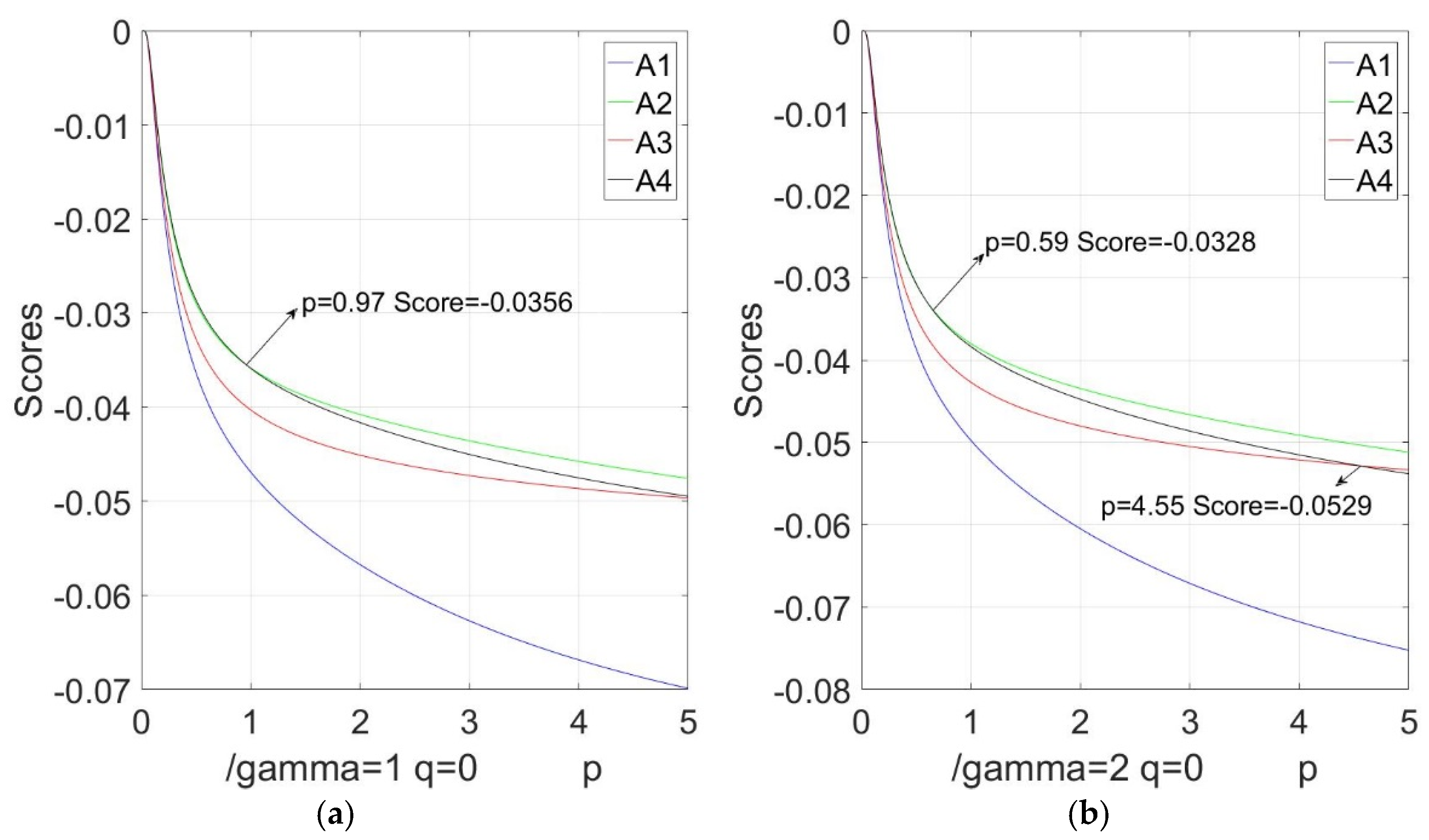
(1) From Table 11 and Figure 1 and Figure 2, the best resolution and ordering results of the alternatives are concordant when $\gamma >1.33$ and $p,q$ are given in the NIFHWHM or NIFHWGHM operators. When $\gamma \le 1.33$ and there is a zero in $p$ and $q$, the ordering results are different.

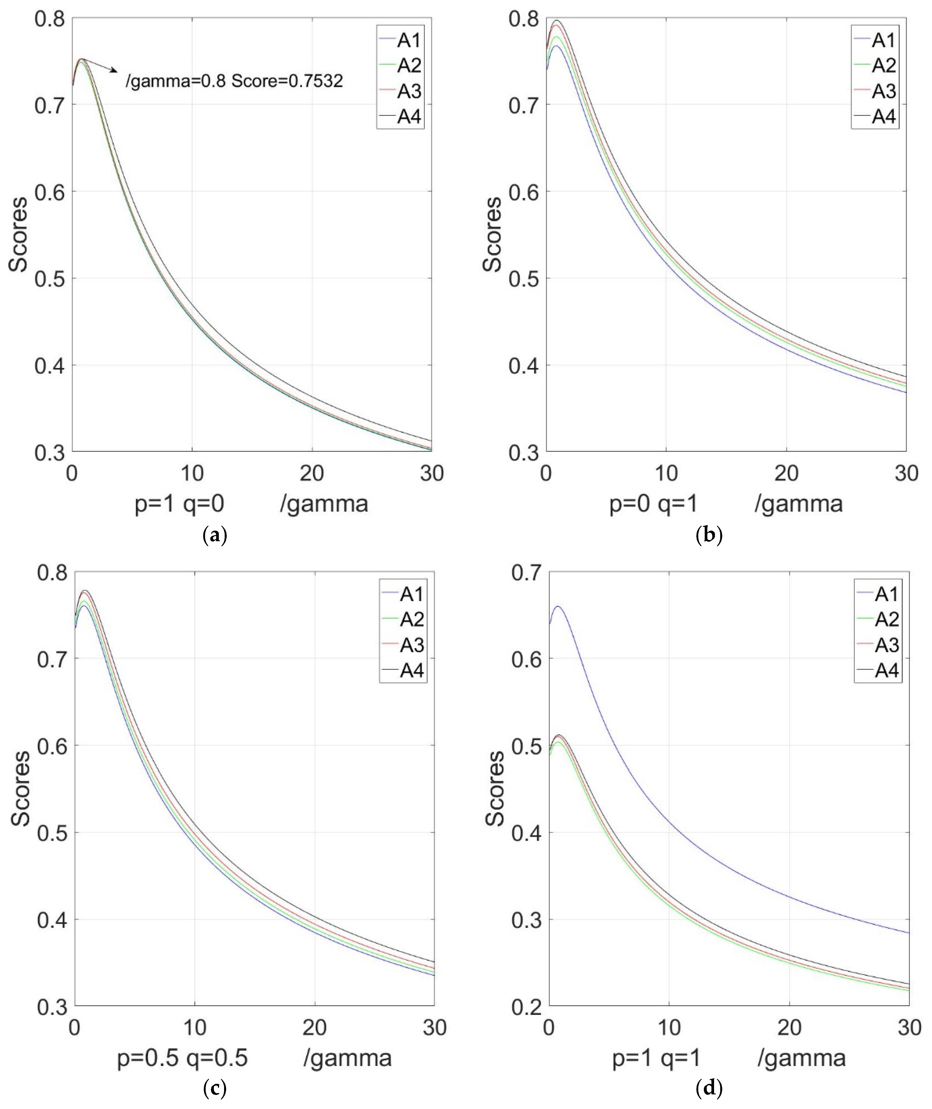
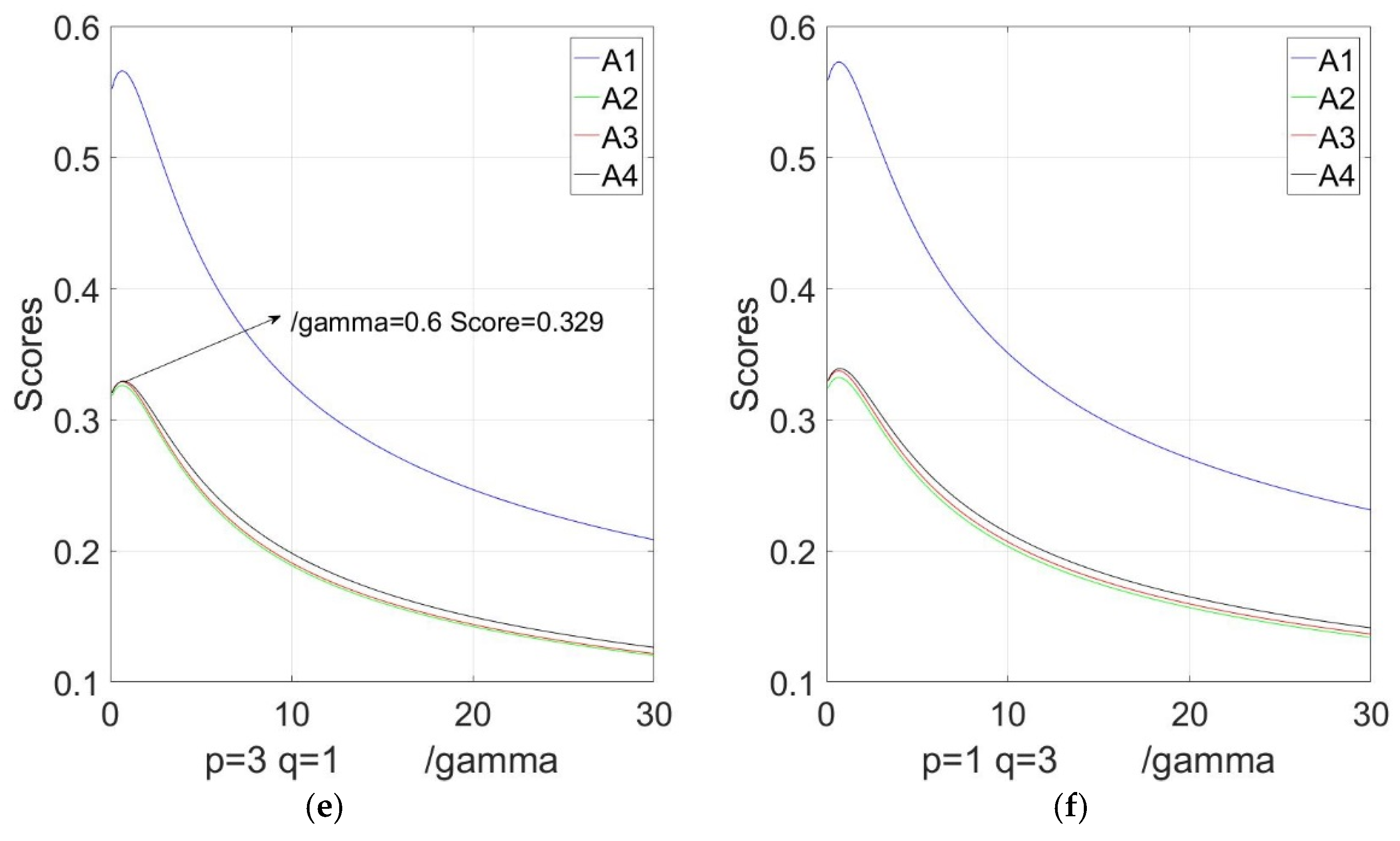
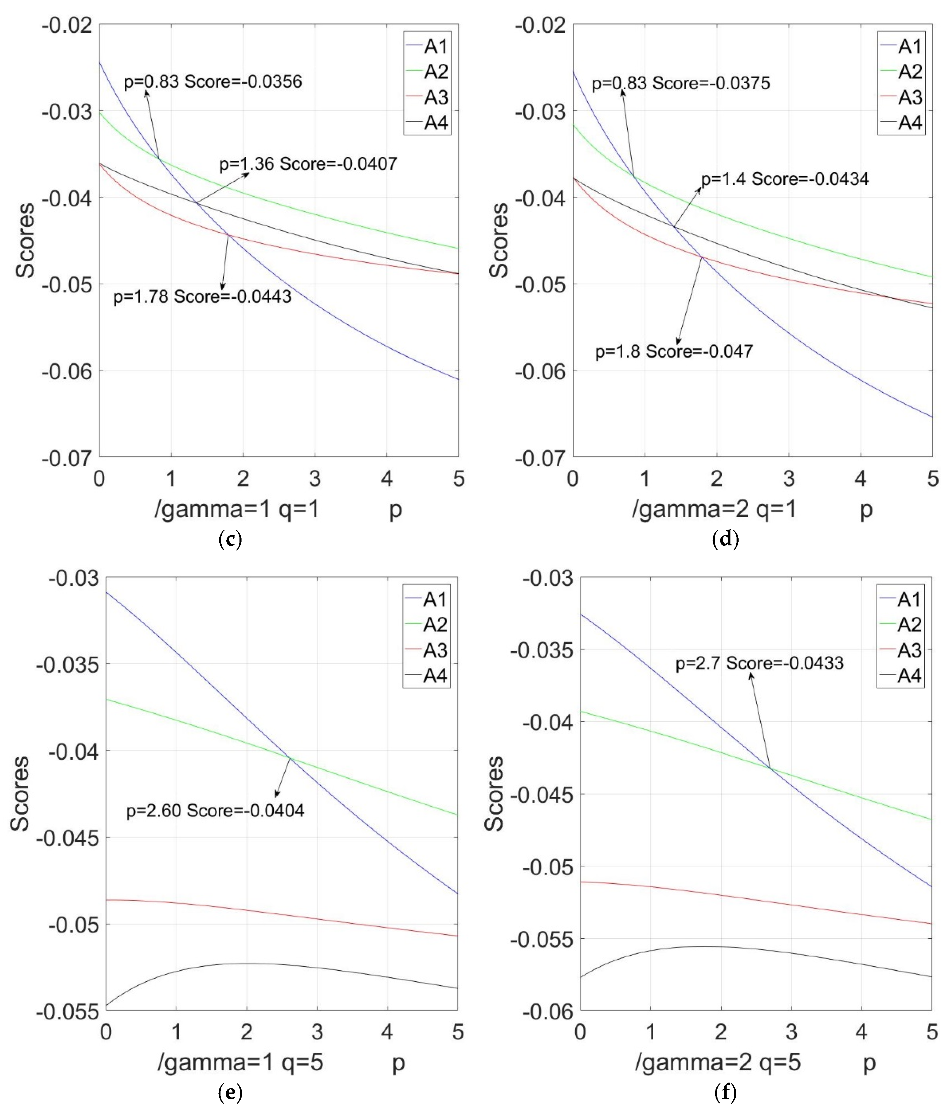
(2) From Figure 3 and Figure 4, we can see that when $\gamma ,q$ are given in the NIFHWHM or NIFHWGHM operators and $p$ takes the values of the different intervals, the best resolution and the orderings are different. For example, with the NIFHWHM operator, when $\gamma =1,q=1$, $p\in \left(0,0.83\right]$, the ranking is $A_1\succ A_2\succ A_4\succ A_3$; when $p\in \left(0.83,\mathrm{0.1.36}\right]$, the ranking is $A_2\succ A_1\succ A_4\succ A_3$; when $p\in \left(1.36,1.78\right]$, the ranking is $A_2\succ A_4\succ A_1\succ A_3$; and when $p\in \left(1.78,5\right]$, the ranking is $A_2\succ A_4\succ A_3\succ A_1$. Additionally, we notice that when $p\in \left(0.83,\mathrm{0.1.36}\right]$, the best one is $A_1$; when $p\in \left(0.83,5\right]$, the best one is $A_2$.

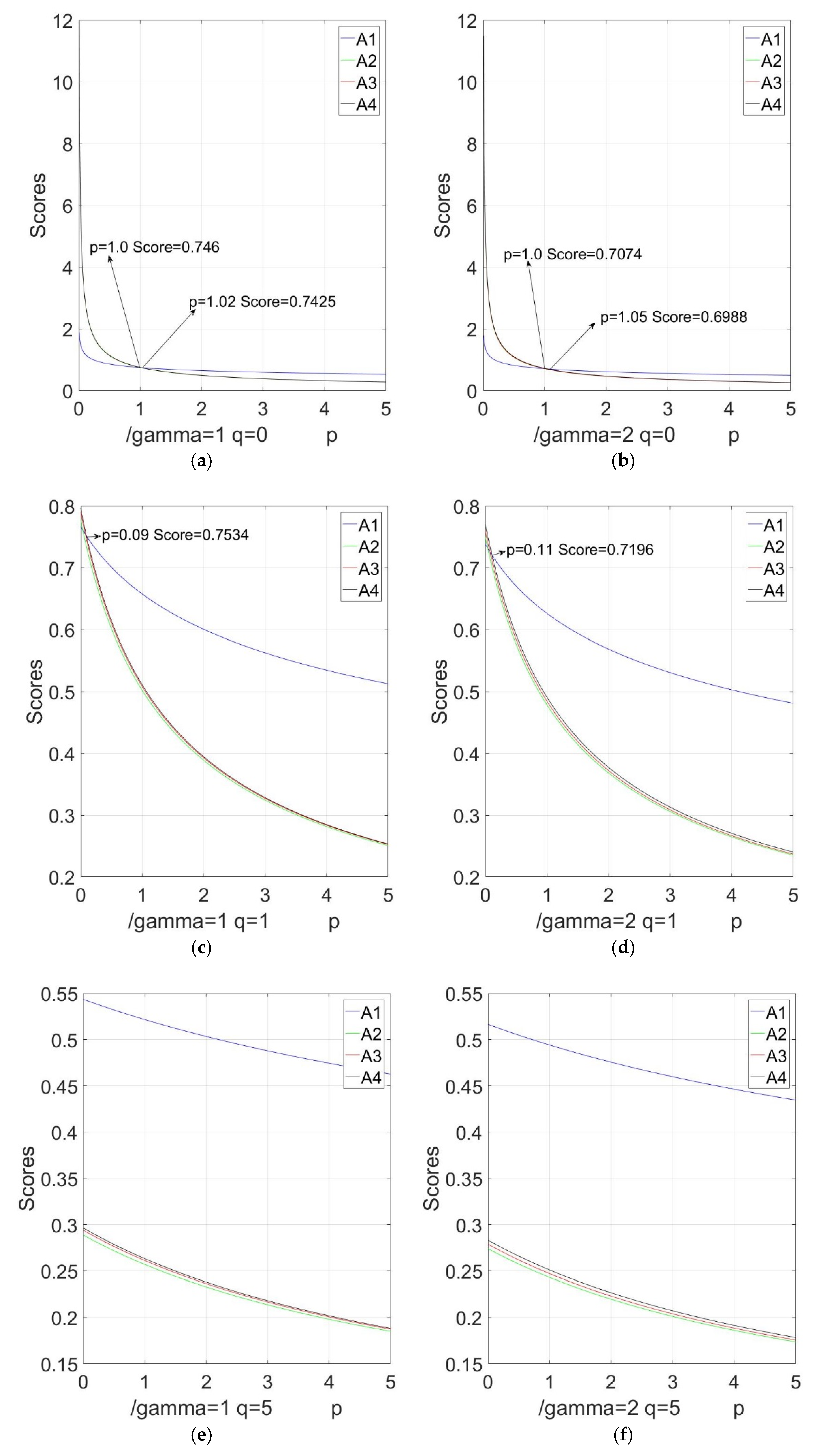
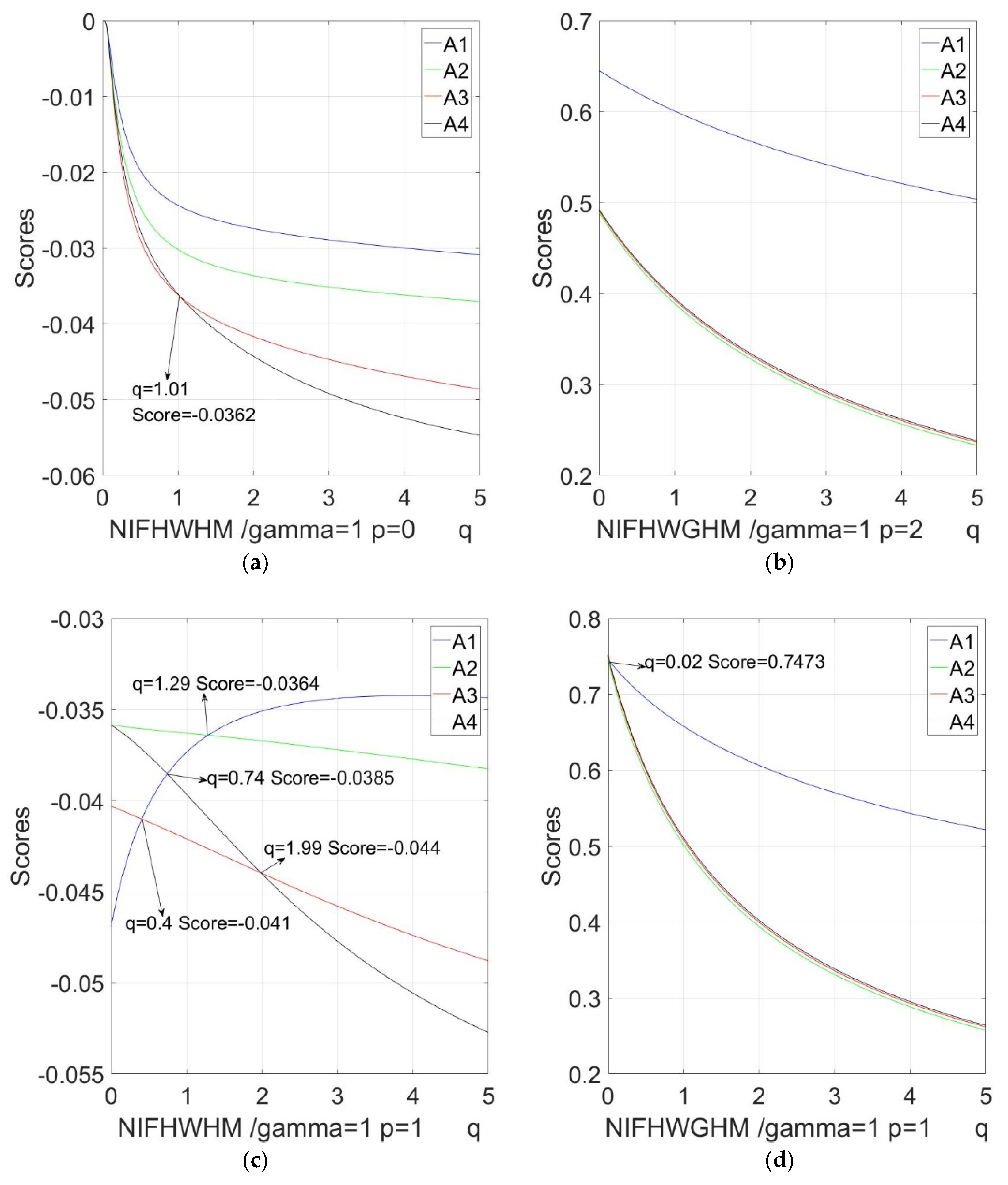
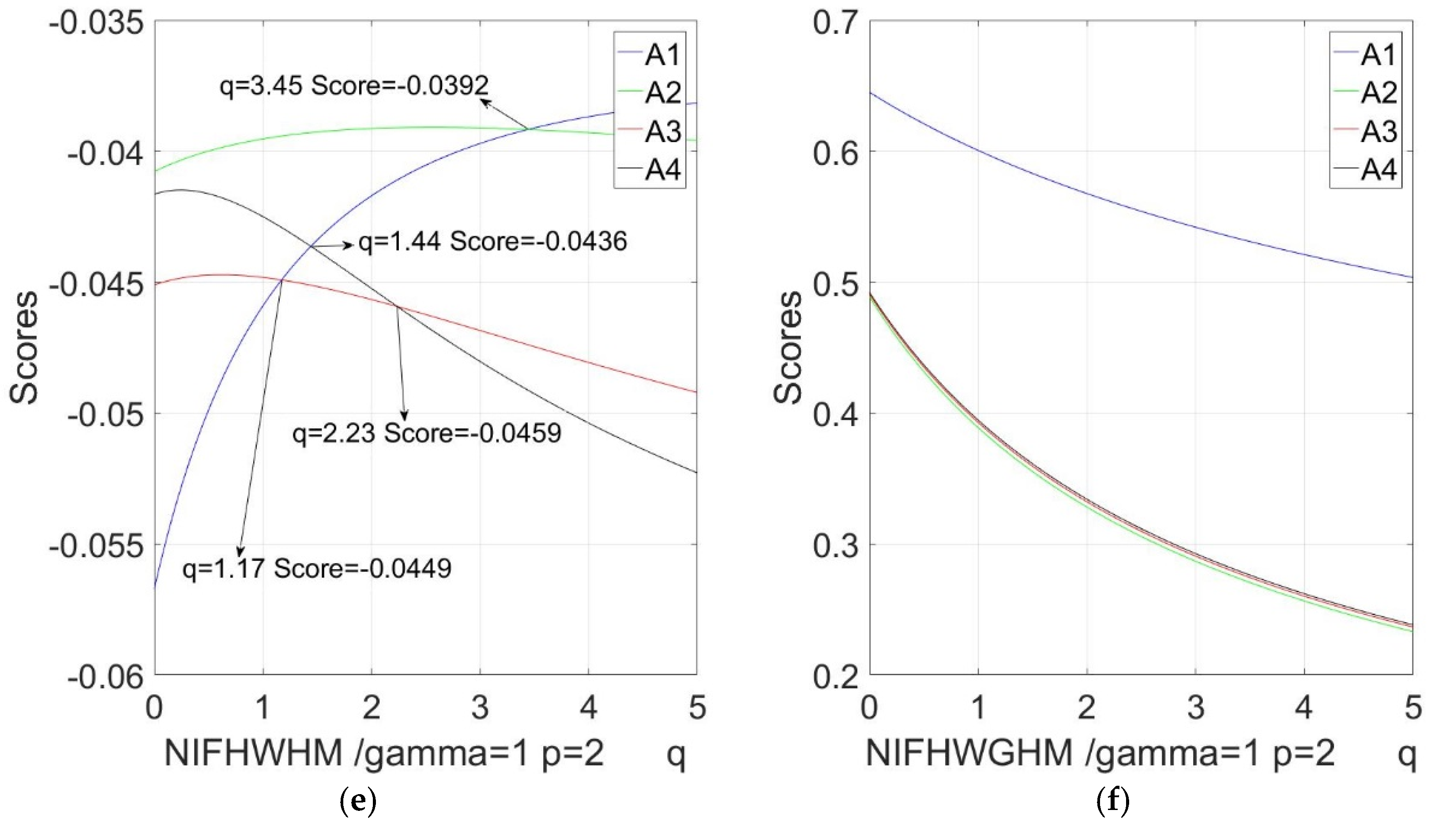
(3) Figure 5 shows that sensitivity of the parameter $q$ is similar to the parameter $p$, but the influence of the value of $q$ is less in the NIFHWGHM operator. As long as $q>0.11$, the rankings are concordant $A_1\succ A_4\succ A_3\succ A_2$.

(4) From Table 11 and Figure 1, Figure 2, Figure 3, Figure 4 and Figure 5, on the whole, the score function values of the NIFHWHM or NIFHWGHM operators become smaller when the parameters $\gamma$, $p$, and $q$ increase. Therefore, the parameters $\gamma$, $p$, and $q$ play crucial roles in the MCGDM procedure. In practical cases, the decision makers can take different values of the parameter, for example, the bigger parameter values are chosen by decision experts who are pessimistic, while smaller parameter values are adopted when decision experts take an optimistic view of the decision results. For convenience, we can assign $\gamma =p=q=1$ or $\gamma =2,p=q=1$; especially, when $\gamma =p=q=1$, the mathematical calculation can be simplified.

In a word, based on the generalized parameters $\gamma$, $p$, and $q$ in the NIFHWHM operator and NIFHWGHM operator, the new method in this paper can offer more flexible or reliable decision-making resolutions. Moreover, the reasonable and best alternative can be properly obtained on the basis of the practical MAGDM problems, namely, the new method can offer a powerful and effective mathematic tool for the MAGDM under uncertainty.

6.3. Comparison Analysis

6.3.1. A Comparison with Decision-Making Methods Using Triangular and Trapezoidal Intuitionistic Fuzzy Information

For further comparison of the rationality and comprehensiveness of the new MCGDM approach in this paper, a prospect value determination method with the TraIFNs [17] and a method with TriIFNs [25] are applied in this section to deal with the aforementioned example. Thus, we need transform the TraIFNs and TriIFNs by the transformation method in [33], which is shown in

Table 12. Transformation method of the normal intuitionistic fuzzy number (NIFN), trapezoidal IFN (TraIFN), and triangular IFN (TriIFN).

NIFN	TraIFN	TriIFN
$\langle \left(\alpha ,\sigma \right),\mu ,v\rangle$	$\begin{array}{c}\langle \left(a_1,a_2,a_3,a_4\right),\left(b_1,b_2,b_3,b_4\right);\mu ,v\rangle \\ a_1=\alpha -2.5\sigma b_1=\alpha -3\sigma \\ a_2=\alpha -1.5\sigma b_2=\alpha -2\sigma \\ a_3=\alpha +1.5\sigma b_3=\alpha +2\sigma \\ a_4=\alpha +2.5\sigma b_4=\alpha +3\sigma \end{array}$	$\begin{array}{c}\langle \left(a,b,c\right);\mu ,v\rangle \\ a=\alpha -3\sigma ,b=\alpha ,c=\alpha +3\sigma \end{array}$

. According to Table 12, the information $r_{ij}^k=\langle \left(a_{ij}^k,{\sigma }_{{}_{ij}}^k\right);{\mu }_{{}_{ij}}^k,v_{{}_{ij}}^k\rangle$ from each expert is also transformed into the TraIFNs and the TriIFNs. Moreover, the normalization method of the TraIFN and TriIFN decision matrix is presented as follows.

$$\stackrel{\sim }{r_{ij}^k}=\{\begin{array}{c}\langle (\frac{a_{ij}^k}{c_j^{k+}},\frac{b_{ij}^k}{c_j^{k+}},\frac{c_{ij}^k}{c_j^{k+}});{\mu }_{{}_{ij}}^k,v_{{}_{ij}}^k\rangle \\ \langle (\frac{{a1}_{ij}^k}{{a4}_j^{k+}},\frac{{a2}_{ij}^k}{{a4}_j^{k+}},\frac{{a3}_{ij}^k}{{a4}_j^{k+}},\frac{{a4}_{ij}^k}{{a4}_j^{k+}}),(\frac{{b1}_{ij}^k}{{b4}_j^{k+}},\frac{{b2}_{ij}^k}{{b4}_j^{k+}},\frac{{b3}_{ij}^k}{{b4}_j^{k+}},\frac{{b4}_{ij}^k}{{b4}_j^{k+}});{\mu }_{{}_{ij}}^k,v_{{}_{ij}}^k\rangle \end{array}j\in B$$

where $B$ is benefit attributes set.

From

Table 13. Comparison of the ranking results by methods in [17,25,30].

Method	Measure	A1	A2	A3	A4	Ranking
Value determination in [17]	Prospect value function	−0.291	−0.137	−0.185	−0.243	A2>A3>A4>A1
Tended TODIM in [25]	Closeness coefficient	0.786	0.279	0.491	0.431	A2>A4>A3>A1
TOPSIS in [30]	Closeness coefficient	0.489	0.282	0.798	0.427	A2>A4>A1>A3
Method in this paper	Score function	−0.035	−0.034	−0.040	−0.037	A2>A1>A4>A31
		−0.037	−0.036	−0.042	−0.038	A2>A1>A4>A32
		−0.039	−0.038	−0.044	−0.042	A2>A1>A4>A33

¹ Parameter $\gamma =0.5,p=q=1$ by NIFHWHM operator; ² Parameter $\gamma =1,p=q=1$ by NIFHWHM operator; ³ Parameter $\gamma =2,p=q=1$ by NIFHWHM operator.

, it can be seen that the best resolution of the three methods is $A_2$, but the ordering results are different for these methods. The proposed method of this paper takes into account the interrelations between input data, and it is more practical than the methods in [17,25,30]. The reason is that there are many normal random factors under the social and economic environment. Furthermore, in light of central limit theorem, the limit distribution of the sum of random variables is a normal distribution. However, the TriIFNs and TraIFNs cannot better depict the laws of normal distribution and accurately express corresponding normal random phenomena. Therefore, compared with the TriIFNs and TraIFNs, the NIFNs can better describe the decision problems with normal distribution information and can more realistically express the uncertainty information, and the MCGDM approach in this paper is more reliable and reasonable to aggregate the normal distribution information than the methods in [17,25,30].

6.3.2. A Comparison with Decision-Making Methods Using the NIFNs

In order to study the advantages of the MCGDM approach in this paper, three methods were applied to deal with the problem in the aforementioned example, and the aggregation results can be seen in

Table 14. Comparison of the ranking results by methods in [34,36,62].

Method	Measure	A1	A2	A3	A4	Ranking
MADM method by NIFI operator in [34]	Score function	0.486	0.779	0.491	0.531	A2>A4>A3>A1
MADM method by NIFBM operator in [36]	Score function	0.476	0.482	0.471	0.467	A2>A1>A3>A4
VIKOR-based dynamic method in [62]	Compromise value function	0.998	0.003	0.775	0.698	A2>A4>A3>A1
Method in this paper	Score function	−0.035	−0.034	−0.040	−0.037	A2>A1>A4>A31
		−0.037	−0.036	−0.042	−0.038	A2>A1>A4>A32
		−0.039	−0.038	−0.044	−0.042	A2>A1>A4>A33
		−0.044	−0.035	−0.041	−0.037	A2>A1>A4>A34

¹ Parameter $\gamma =0.5,p=q=1$ by NIFHWHM operator; ² Parameter $\gamma =1,p=q=1$ by NIFHWHM operator; ³ Parameter $\gamma =2,p=q=1$ by NIFHWHM operator; ⁴ Parameter $\gamma =1,p=0,q=1$ by NIFHWHM operator.

.

From Table 14, we can observe that the best alternatives are all $A_2$, but the solution ordering results are completely different for four methods, which can all tackle NIF information. We consider that there are wide interrelationships among the attributes or relationships between input argument and itself in practical MAGDM problems. Moreover, the new method in this paper considers the interrelationship factor between input arguments or between input argument and itself. Therefore, compared with two methods in [34,62], the ranking results from the new method in this paper is more effective and more reasonable.

In addition, if $q=0$ or $p=0$, then the interrelationships did not exist in the new method in this paper. In the aforementioned example, we can obtain the aggregation ordering results, namely, the relationships between arguments or among the attributes are not considered in the method proposed in this paper. The solution ordering result is the same as that using the methods in [34,62], consequently, this verifies the different ordering results.

Furthermore, for a group of attributes $c_i\left(i=1,2,\cdots ,n\right)$ and a collection of input arguments $a_i\left(i=1,2,\cdots ,n\right)$, the method in [36] also takes into account the relationships between any pair of attributes $c_i$ and $c_j$ $\left(i\ne j\right)$ or between any pair of input arguments $a_i$ and $a_j$$\left(i\ne j\right)$, but it neglects the correlation between input argument $a_i$ and itself or between the attribute $c_i$ and itself. Considering that the correlation between $a_i$ and $a_j$$\left(i\ne j\right)$ or between $c_i$ and $c_j$ $\left(i\ne j\right)$ is equal to the correlation between $a_i$ and $a_j$$\left(i\ne j\right)$ or between $c_i$ and $c_j$ $\left(i\ne j\right)$, the method in [36] deals with it separately and brings about redundancy. Therefore, compared with the method in [36], the new method in this paper not only considers relationships between the input arguments or the attributes, but also takes into account the correlation between input argument and itself. Furthermore, interrelationships between input arguments are tackled once.

7. Conclusions

In this work, enlightened by Heronian mean, we significantly investigated a family of generalized fuzzy HM operators based on Hamacher operation for NIFNs, including NIFHHM, NIFHWHM, NIFHGHM, and NIFHWGHM operators, and we discuss various properties of the proposed operators which have the desirable quality of not only dealing with the normal intuitionistic fuzzy information, but also considering the correlations of two input arguments once. Therefore, the new proposed operators do not result in redundancy, and these operators also take into account the interrelationship between input argument and itself at the same time. Furthermore, we have manifested that the operators related to Hamacher operation generalize the operators based on the algebraic or Einstein operational rules, and they are more flexible to extend the choice scope of decision makers. On the basis of the developed operators, a new MCGDM approach is introduced in order to deal with normal intuitionistic fuzzy number information. The advantages of this new method are that: (1) it is more reliable and reasonable to aggregate the normal distribution information under the normal intuitionistic fuzzy numbers environment; (2) it offers an effective and powerful mathematic tool for the MAGDM under uncertainty and can provide more reliable and flexible aggregation results in decision making; (3) it not only considers relationships between the input arguments or the attributes, but also takes into account the correlation between input argument and itself or the interrelations between the attribute and itself, furthermore, interrelationships between input arguments or the attributes are tackled once. The new methods provide some reasonable and reliable MCGDM aggregation operators, which broaden the selection scope of the decision makers and offer theory evidence for the MCGDM methods. Meanwhile, the proposed methods solve the interaction of the different criteria or input arguments and do not bring about redundancy of the mathematical calculation. Lastly, an application example revealed that the developed approach is effective and practical by the comparison with other methods. In further research, it is important to investigate how to determine the weights and how to transform other types of fuzzy numbers into the NIFNs, and it is essential to study the application of the proposed operators in wide fields, such as uncertain programming, cluster analysis, pattern recognition, and so on.