DSmT Decision-Making Algorithms for Finding Grasping Configurations of Robot Dexterous Hands

Institute of Solid Mechanics of the Romanian Academy, 010141 Bucharest S1, Romania
*
Author to whom correspondence should be addressed.
Symmetry 2018, 10(6), 198; https://doi.org/10.3390/sym10060198
Submission received: 14 May 2018
/
Revised: 27 May 2018
/
Accepted: 29 May 2018
/
Published: 1 June 2018
(This article belongs to the Special Issue Algebraic Structures of Neutrosophic Triplets, Neutrosophic Duplets, or Neutrosophic Multisets)
Abstract
:In this paper, we present a deciding technique for robotic dexterous hand configurations. This algorithm can be used to decide on how to configure a robotic hand so it can grasp objects in different scenarios. Receiving as input, several sensor signals that provide information on the object’s shape, the DSmT decision-making algorithm passes the information through several steps before deciding what hand configuration should be used for a certain object and task. The proposed decision-making method for real time control will decrease the feedback time between the command and grasped object, and can be successfully applied on robot dexterous hands. For this, we have used the Dezert–Smarandache theory which can provide information even on contradictory or uncertain systems.
1. Introduction
The purpose of autonomous robotics is to build systems that can fulfill all kinds of tasks without human intervention, in different environments which were not specially build for robot interaction. A major challenge for this autonomous robotics field comes from high uncertainty within real environments. This is because the robot designer cannot know all the details regarding the environment. Most of the environment parameters are unknown, the position of humans and objects cannot be previously anticipated and the motion path might be blocked. Beside these, the accumulated sensor information can be uncertain and error prone. The quality of this information is influenced by noise, visual field limitations, observation conditions, and the complexity of interpretation technique.
The artificial intelligence and the heuristic techniques were used by many scientists in the field of robot control [1] and motion planning. Regarding grasping and object manipulations, the main research activities were to design a mechanism for hand [2,3,4] and dexterous finger motion [5], which are a high complexity research tasks in controlling robotic hands.
Currently, in the research area of robotics, there is a desire to develop robotic systems with applications in dynamic and unknown environments, in which human lives would be at risk, like natural or nuclear disaster areas, and also in different fields of work, ranging from house chores or agriculture to military applications. In any of these research areas, the robotic system must fulfill a series of tasks which implies object manipulation and transportation, or using equipment and tools. From here arises the necessity of development grasping systems [6] to reproduce, as well as possible human hand motion [7,8,9].
To achieve an accurate grasping system, a grasp taxonomy of the human hand was analyzed by Feix et al. [10] who found 33 different grasp types, sorted by opposition type, virtual finger assignments; type in terms of power, precision, or intermediate grasp; and the position of the thumb. While Alvarez et al. [11] researched human grasp strategies within grasp types, Fermuller et al. [12] focused on manipulation action for human hand on different object types including hand pre-configuration. Tsai et al. [13] found that classifying objects into primitive shapes can provide a way to select the best grasping posture, but a general approach can also be used for hand–object geometry fitting [14]. This classification works well for grasping problems in constrained work space using visual data combined with force sensors [15] and also for under-actuated grasping which uses rotational stiffness [16]. However, for unknown objects, scientists found different approaches to solve the hand grasping problem. Choi et al. [17] used two different neural networks and data fusion to classify objects, Seredynski et al. [18] achieved fast grasp learning with probabilistic models, while Song et al. [19] used a tactile-based blind grasping along with a discrete-time controller. The same approach is used by Gu et al. [20] which proposed a blind haptic exploration of unknown objects for grasp planning of dexterous robotic hand. Using grasping methods, Yamakawa et al. [21] developed a robotic hand for knot manipulation, while Nacy et al. [22] used artificial neural network algorithms for slip prevention and Zaidi et al. [23] used a multi-fingered robot hand to grasp 3D deformable objects, applying the method on spheres and cubes.
While other scientists developed grasping strategies for different robotic hands [21,22,23], an anthropomorphic robotic hand has the potential to grasp regular objects of different shapes and sizes [24,25], but selecting the grasping method for a certain object is a difficult problem. A series of papers have approached this problem by developing algorithms for classifying the grasping by the contact points [26,27]. These algorithms are focused on finding a fix number of contact areas without taking into consideration the hand geometry. Other methods developed grasping systems for a certain robotic hand architecture, scaling down the problem to finding a grasping method with the tip of the fingers [27]. These methods are useful in certain object manipulation, but cannot be applied for a wide range of objects because it does not provide a stable grasping due to the face that it is not used, the finger’s interior surface or the palm of the hand. A method for filtering the high number of hand configurations is to use predefined grasping hand configurations. Before grasping an object, humans, unconsciously simplify the grasping action, choosing one of the few hand positions which match the object’s shape and the task to accomplish. In the scientific literature there are papers which have tried to log in the positioning for grasping and taxonomy, and one of the most known papers is [28]. Cutkosky and Weight [29] have extended Napier’s [28] classification by adding the required taxonomy in the production environment, by studying the way in which the weight and geometry of the object affects choosing the grasping positioning. Iberall [30] has analyzed different grasping taxonomies and generalized them by using the virtual finger concept. Stransfield [31] has chosen a simpler classification and built a system based on rules which provided a grasping positioning set, starting from a simplified description of the object gained from a video system.
The developed algorithm presented in this paper has the purpose to determine the grasping position according to the object’s shape. To prove the algorithm’s efficiency we have chosen three types of objects for grasping: cylindrical, spherical, and prismatic. For this, we start from the hypothesis that the environment data are captured through a stereovision system [32] and a Kinect sensor [33]. On this data, which the two system observers provide, we apply a template matching algorithm [34]. This algorithm will provide a matching percentage of the object that needs to be grasped with a template object. Thus, each of the two sources will provide three matching values, for each of the three grasping types. These values represent the input for our detection algorithm, based of Dezert–Smarandache Theory (DSmT) [35] for data fusion. This algorithm has as input data from two or multiple observers and in the first phase they are processed through a process of neutrosofication which is similar with the fuzzification process. Then, the neutrosophic observers’ data are passed through an algorithm which applies the classic DSm theory [35] in order to obtain a single data set on the system’s states, by combining the observers’ neutrosophic values. On this obtained data set, we apply the developed DSmT decision-making algorithm that decides on the category from which the target object is part of. This decision facilitates the detection–recognition–grasping process which a robotic hand must follow, obtaining in the end a real-time decision that does not stop or delay the robot’s task.
In recent years, using more sensors for a certain applications and then using data fusion is becoming more common in the military and nonmilitary research fields. The data fusion techniques combine the information received from different sensors with the purpose of eliminating disturbances and to improve precision compared to the situations when a single sensor is used [36,37]. This technique works on the same principle used by humans to feel the environment. For example, a human being cannot see over the corner or through vegetation, but with his hearing he can detect certain surrounding dangers. Beside the statistical advantage build from combining the details for a certain object (through redundant observations), using more types of sensors increases the precision with which an object can be observed and characterized. For example, an ultrasonic sensor can detect the distance to an object, but a video sensor can estimate its shape, and combining these two information sources will provide two distinct data on the same object.
The evolution on the new sensors, the hardware’s processing techniques and capacity improvements facilitate more and more the real time data fusion. The latest progress were made in the area of computational and detection systems, and provide the ability to reproduce, in hardware and software, the data fusion capacity of humans and animals. The data fusion systems are used for target tracking [38], automatic target identification [39], and automated reasoning applications [40]. The data fusion applications are widespread, ranging from the military [41] applications (target recognition, autonomous moving vehicles, distance detection, battlefield surveillance, automatic danger detection) to civilian application (monitoring the production processes, complex tools maintenance based on certain conditions, robotics [42], and medical applications [43]). The data fusion techniques undertake classic elements like digital signal processing, statistical estimation, control theory, artificial intelligence, and numeric methods [44].
Combined data interpretation requires automated reasoning techniques taken from the area of artificial intelligence. The purpose of developing the recognition based systems, was to analyze issues like the data gathering context, the relationship between observed entities, hierarchical grouping of targets or objects and to predict future actions of these targets or entities. This kind of reasoning is encountered in humans, but the automated reasoning techniques can only closely reproduce it. Regardless of the used technique, for a knowledge based system, three elements are required: one or more reasoning diagrams, an automated evaluation process and a control diagram. The reasoning diagrams are techniques of facts representation, logical relations, procedural knowledge, and uncertainty. For these techniques, uncertainty from the observed data and from the logical relations can be represented using probabilities, fuzzy theory [45,46], Dempster–Shafer [47] evidence intervals or other methods. Dezert–Smarandache theory [35] comes to extend these methods, providing advanced techniques of uncertainty manipulation. The automated reasoning system’s developing purpose is to reproduce the human capability of reasoning and decision making, by specifying rules and frames that define the studied situation. Having at hand an information database, an evaluation process is required so this information can be used. For this, there are formal diagrams developed on the formal logic, fuzzy logic, probabilistic reasoning, template based methods, case based reasoning, and many others. Each of these reasoning diagrams has a consistent internal formalism which describes how to use the knowledge database for obtaining the final conclusion. An automated reasoning system needs a control diagram to fulfill the thinking process. The used techniques include searching methods, systems for maintaining the truth based on assumptions and justifications, hierarchical decomposition, control theory, etc. Each of these methods has the purpose of controlling the reasoning evolution process.
The results presented in this paper, were obtained using the classic Dezert–Smarandache theory (DSmT) to combine inputs from two different observers that want to classify objects into three categories: sphere, parallelepiped, and cylinder. These categories were chosen to include most of the objects that a manipulator can grasp. The algorithm’s inputs were transformed into belief values of certainty, falsity, uncertainty, and contradiction values. Using these four values and their combinations according to DSmT, we applied Petri net diagram logic for taking decisions on the shape type of the analyzed objects. This type of algorithm has never been used before for real time decision on hand grasping taxonomy. Compared to other algorithms [13,14,15] and methods [16,17,18], ours has the advantage to detect high uncertainties and contradictions which in practice has a very low encounter rate but can have drastic effects on the decision type or robot, because if the object’s shape is not detected properly, then the robot might not be able to grasp it, which can lead to serious consequences. In deciding how to grasp objects, researchers have used different methods to choose the grasping taxonomy using a blind haptic exploration [20] or in different applications for tying knots [21] or grasp deformable objects [23]. Because the proposed algorithm can detect anomalies of contradicting and uncertain input values, we can say that the proposed method transforms the deciding process into a less difficult problem of grasping method [24,25].
2. Objects Grasping and Its Classification
Mechanical hands have been developed to provide the robots with the ability of grasping objects with different geometrical and physical properties [48]. To make an anthropomorphic hand seem natural, its movement and the grasping type must match the human hand.
In this regard, grasping position taxonomy for human hands has been long studied and applied for robotic hands. Seventeen different categories of human hands grasping positions were studied. However, we must consider two important things: the first thing is that these categories are derived from human hand studies, which proves that they are more flexible and able to perform a multitude of movements than any other robotic hand, so that the grasping taxonomy for robot hands can be only a simple subset of the human hand. The second is that the human behavior studies of real object grasping have shown some differences between the real observations and the classified properties [49].
In conclusion, any proposed taxonomy is only a reference point which the robot hand must attain. Below the most used grasping positions are described (extracted from [50]), which should be considered when developing an able robotic hand:
- Power grasping: The contact with the objects is made on large surfaces of the hand, including hand phalanges and the palm of the hand. For this kind of grasping, high forces can be exerted on the object.
- Spherical grasping: used to grasp spherical objects;
- Cylindrical grasping: used to grasp long objects which cannot be completely surrounded by the hand;
- Lateral grasping: the thumb exerts a force towards the lateral side of the index finger.
- Precision grasping: the contact is made only with the tip of the fingers.
- Prismatic grasping (pinch): used to grasp long objects (with small diameter) or very small. Can be achieved with two to five fingers.
- Circular grasping (tripod): used in grasping circular or round objects. Can be achieved with three, four, or five fingers.
- No grasping:
- Hook: the hand forms a hook on the object and the hand force is exerted against an external force, usually gravity.
- Button pressing or pointing
- Pushing with open hand.
3. Object Detection Using Stereo-Vision and Kinect Sensor
Object recognition in artificial sight represents the task of searching a certain object in a picture or a video sequence. This problem can be approached as a learning problem. At first, the system is trained with sample images which belong to the target group, the system being taught to spot these among other pictures. Thus, when the system receives new images, it can ‘feel’ the presence of the searched object/sample/template.
Template matching is a techniques used to sort objects in an image. A model is an image region, and the goal is to find instances of this model in a larger picture. The template matching techniques represent a classic approach for localization problems and object recognition in a picture. These methods are used in applications like object tracking, image compression, stereograms, image segmentation [52], and other specific problems of artificial vision [53].
Object recognition is very important for a robot that must fulfill a certain task. To complete its task, the robot must avoid obstacles, obtain the size of the object, manipulate it, etc. For the case of detected object manipulation, the robot must detect the object’s shape, size, and position in the environment. The main methods for achieving the depth information use stereoscopic cameras, laser scanners, and depth cameras.
To achieve the proposed decision-making algorithm, we assumed that the environment information is captured with a stereoscopic system and a Kinect sensor.
Stereovision systems [32] represents a passive technique of achieving a virtual 3D image of the environment in which the robot moves, by matching the common features of an image set of the same scene. Because this method works with images, it needs a high computational power. The depth information can be noisy in certain cases, because the method depends on the texture of the environment objects and on the ambient light.
Kinect [33] is a fairly easy to obtain platform, which makes it widespread. It uses a depth sensor based on structured light. By using an ASIC board, the Kinect sensor generates a depth map on 11 bits with a resolution of 640 × 480 pixels, at 30 Hz. Given the price of the device, the information quality is pretty good, but it has both advantages and disadvantages, meaning that the depth images contain areas where the depth reading could not be achieved. This problem appears from the fact that some materials do not reflect infrared light. When the device is moved really fast, like any other camera, it records blurry pictures, which also leads to missing information from the acquired picture.
4. Neutrosophic Logic and DSm Theory
4.1. Neutrosophic Logic
The neutrosophic triplet (truth, falsity, and uncertainty) idea appeared in 1764 when J.H. Lambert investigates a witness credibility which was affected by the testimony of another person. He generalized Hooper’s rule of sample combination (1680), which was a non-Bayesian approach for finding a probabilistic model. Koopman in 1940 introduces the low and high probability, followed by Good and Dempster (1967) who gave a combination rule of two arguments. Shafer (1976) extended this rule to Dempster–Shafer Theory for trust functions by defining the trust and plausibility functions and using the inference rules of Dempster for combining two samples from two different sources. The trust function is a connection between the fuzzy reasoning and probability. Dempster–Shafer theory for trust functions is a generalization of Bayesian probability (Bayes 1760, Laplace 1780). It uses the mathematical probability in a more general way and it is based on the probabilistic combination of artificial intelligence samples.
Lambert one said that “there is a chance p that the witness can be trustworthy and fair, a chance q that he will be deceiving and a chance 1-p-q that he will be indifferent”. This idea was taken by Shafer in 1986 and later, used by Smarandache to further develop the neutrosophic logic [54,55].
4.1.1. Neutrosophic Logic Definition
A logic in which each proposition has its percentage of truth in a subset T, its percentage of uncertainty in a subset I, and its percentage of falsity in a subset F is called neutrosophic logic [54,55].
This paper extends the general structure of the neutrophic robot control (RNC), known as the Vladareanu–Smarandache method [55,56,57] for the robot hybrid force-position control in a virtual platform [58,59], which applies neutrosophic science to robotics using the neutrosophic logic and set operators. Thus, using two observers, a stereovision system and a Kinect sensor, will provide three matching values for DSmT decision-making algorithms. A subset of truth, uncertainty and falsity is used instead of a single number because in many cases one cannot know with precision the percentage of truth or falsity, but these can be approximated. For example, a supposition can be 30% to 40% true and 60% to 70% false [60].
4.1.2. Neutrosophic Components Definition
Let be three standard or non-standard subsets of with
and
The T, I, and F sets are not always intervals, but can be subsets: discrete or continuum; with a single element; finite or infinite (the elements are countable or uncountable); subsets union or intersection. Also, these subsets can overlap, and the real subsets represent the relative errors in finding the t, i, and f values (when the T, I, and F subsets are reduced to single points).
T, I, and F are called the neutrosophic components and represent the truth, uncertainty, and falsity values, when referring to neutrosophy, neutrosophic logic, neutrosophic sets, neutrosophic probability, or neutrosophic statistics.
This representation is closer to the human reasoning and defines knowledge imprecision or linguistic inaccuracy received from different observers (this is why T, I, and F are subsets and can be more that a set of points), the uncertainty given by incomplete knowledge or data acquisition errors (for this we have the set I) and the vagueness caused by missing edges or limits.
4.2. Dezert–Smarandache Theory (DSmT)
To develop artificial cognitive systems a good management of sensor information is required. When the input data are gathered by different sensors, according to the environment certain situations may appear when one of the sensors cannot give correct information or the information is contradictory between sensors. To resolve this issue a strong mathematical model is required, especially when the information is inaccurate or uncertain.
The Dezert–Smarandache Theory (DSmT) [53,54,60] can be considered an extension of Dempster–Shafer theory (DST) [46]. DSmT allows information combining, gathered from different and independent sources as trust functions. DSmT can be used for solving information fusion on static or dynamic complex problems, especially when the information differences between the observers are very high.
DSmT starts by defining the notion of a DSm free model, denoted by and says that is a set of exhaustive elements , which cannot overlap. This model is free because there are no other suppositions over the hypothesis. As long as the DSm free model is fulfilled, we can apply the associative and commutative DSm rule of combination.
DSm theory [62] is based on defining the Dedekind lattice, known as the hyper power set of frame . In DSmT, is considered a set of n exhaustive elements, without adding other constraints.
DSmT can tackle information samples, gathered from different information sources which do not allow the same interpretation of the set elements. Let be the simple case, made of two assumption, then [54]:
- the probability theory works (assuming exclusivity and completeness assumptions) with basic probability assignments (bpa) such that
- the Dempster–Shafer theory works, (assuming exclusivity and completeness assumptions) with basic belief assignments (bba) such that
- the DSm theory works (assuming exclusivity and completeness assumptions) with basic belief assignment (bba) such that
4.2.1. The Hyperpower Set Notion
One of the base elements of DSm theory is the notion of hyper power set. Let be a finite set (called frame) with n exhaustive elements. The Dedekind lattice, called hyper power set within DSmT frame, is defined as the set of all built statements from the elements of set with the and operators such that:
- If , then and .
- No other element is included in with the exception of those mentioned at 1 and 2.
duals (obtained by changing within expressions the operator with the operator ) is . In there are elements that are dual with themselves. The cardinality of increases with 2n when the cardinality of is n. Generating the hyper power set is close connected with the Dedekind [54,55] known problem of isotone Boolean function set. Because for any finite set , we call the hyper power set of .
The , elements from form the finite set of suppositions/concepts that characterize the fusion problem. represents the free model of DSm and allows working with fuzzy concepts that describe the intrinsic and relative character. This kind of concept cannot be accurately distinguished within an absolute interpretation because of the unapproachable universal truth.
With all of this, there are certain particular fusion problems that imply discrete concepts, where the elements are exclusively true. In this case, all the exclusivity constraints of , must be included in the previous model to properly characterize the truthiness character of the fusion problem and to match reality. For this, the hyper power set is decreased to the classic power set , forming the smallest hybrid DSm model, noted with , and coincides with Shafer’s model.
Besides the problem types that correspond with the Shaffer’s model and those that correspond with the DSm free model , there is an extensive class of fusion problems that include in states, continuous fuzzy concepts and discrete hypothesis. In this case we must take into consideration certain exclusivity constraints and some non-existential constraints. Each fusion hybrid problem is described by a DSm hybrid model with and .
4.2.2. Generalized Belief Functions
Starting from a general frame , we define a transformation associated with an information source like [54]
The m(A) value is called generalized basic belief assignment of A.
The generalized trust and plausibility are defined in the same way as in Dempster–Shafer theory [47]
These definitions are compatible with the classic trust function definition from the Dempster–Shafer theory when is reduced to for fusion problems where the Shafer model can be applied. We still have . To notice that when we work with the free DSm model, we will always have , which is normal [54].
4.2.3. DSm Classic Rule of Combination
When the DSm free model can be applied, the combination rule of two independent sources and that provide information on the same frame with the belief functions and associated to gbba and correspond to the conjunctive consensus of sources. Data combinations are done by using the formula [54]
Because is closed under and operators, this new combination rule guarantees that Is a generalized trust value, meaning that . This rule of combination is commutative and associative and can be used all the time for sources fusion which implies fuzzy concepts. This rule can be extended with ease for combining k > 2 independent information sources [55,56].
Because of the high number of elements in , when the cardinality of increases, the need of computational resources also increases for processing the DSm combination rule. This observation is true only if the core (the set of generalized basic belief assignment for the needed elements) and coincide with , meaning that when and for any . For most practical applications, the and dimensions are much smaller than because the information sources provide most of the time the generalized basic belief assignment for only one subset of hyper power set. This facilitates the DSm classic rule implementation.
Figure 1 presents the DSm combination rule architecture. The first layer is formed by all the generalized basic belief assignment values of the needed elements of . The second layer is made out of all the generalized basic belief assignment values of . Each node from the first layer is connected with each node of the second layer. The output layer is created by combining the generalized basic belief assignment values of all the possible intersections and . If we would have a third source to provide generalized basic belief assignment values , this would have been combined by placing it between the output layer and the second one that provides the generalized basic belief assignment values . Due to the commutative and associative properties of DSm classic rule of combination, in developing the DSm network, a particular order of layers is not required [54].
5. Decision-Making Algorithm
As observed in this paper, according to the object shape and assigned task, grasping is divided into eight categories [63]: spherical grasping, cylindrical grasping, lateral grasp, prismatic grasp, circular grasping, hook grasping, button pressing, and pushing. From these grasping types, the most used ones are cylindrical and prismatic grasping (see Table 1). These can be used in almost any situation and we can say that spherical grasping is a particular grasping of these two. The spherical grasp is used for power grasping, when the contact with the object is achieved with all the fingers’ phalanges and the hand’s palm. This is why a requirement for classification by the shape of the object is needed. Due to the fact that these types are more often encountered, they were taken into consideration for the studied fusion problems.
The fusion problem aims to achieve a classification, by shape of objects to grasp, so that these can match with the other three types of grasping studied. The target objects are classified into three categories: sphere, parallelepiped, and cylinder. For each category, a grasping type is assigned [56].
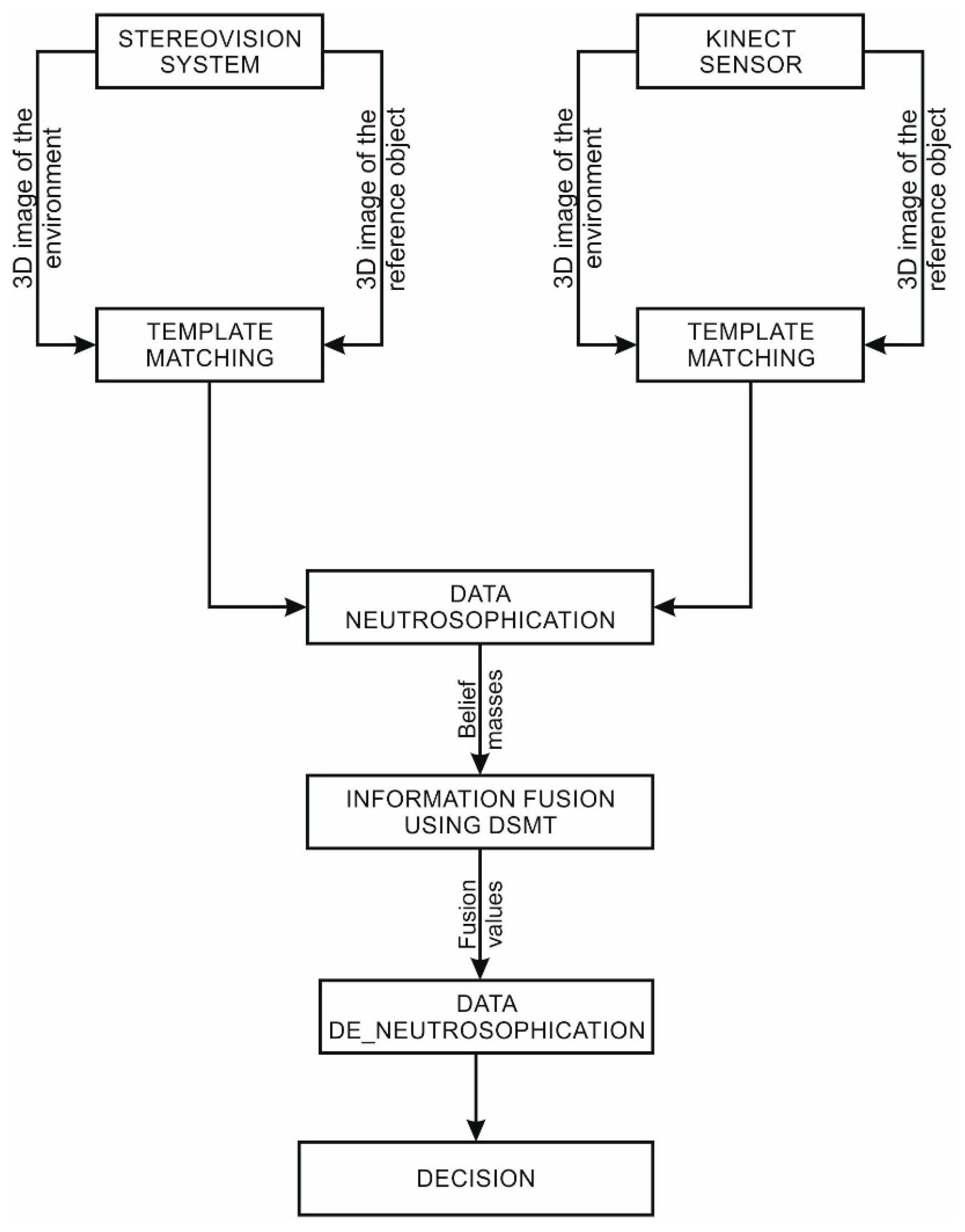
Following the presented theory in Section 4, the information is provided by two independent sources (observers): a stereovision system and a Kinect sensor. The observers are presented in Section 3, and are used to scan the robot’s work environment. By using the information provided by the two observers, a 3D virtual image of the environment is achieved, from which the human operator choses the object to be grasped, thus defining the grasping task that must be achieved by the robot. The 3D image of the object, isolated from the scene, is compared with three templates—formed by similar methods—which represent a sphere, a parallelepiped, and a cylinder. Afterwards, a template matching algorithm is applied to place the object in one of the three categories, with a certain matching percentage. This percentage can vary according to the conditions in which the images are obtained (weak light, object from which the light is reflected, etc.). The data taken from each sensor are then individual processed with a neutrosophication algorithm, with the purpose of obtaining the generalized basic belief assignment values for each hypothesis that can characterize the system. In the next step, having the basic belief assignment values, we combine the data provided by the two observers by using the classic DSm rule of combination. The next step is to apply a deneutrosophication algorithm on the obtained values, to achieve the decision on the shape of the object by placing it into the three categories mentioned above. The entire process is visually represented in Figure 2.
5.1. Data Neutrosophication
Each observer provides a truth percentage for each system’s state. The state set that characterizes the fusion problem is
where Sp = sphere, Pa = parallelepiped, and Cy = cylinder.
To compute the belief values for the hyper power set elements we developed an algorithm based on the neutrosophic logic. The hyper power set is formed by using the method presented in Section 4.2.1 and has the form
The statements of each observer are handled in ways of truth (T), uncertainty (I), and falsity (F), specific to the neutrosophic logic. Due to the fact that , the statements of falsity are not taken into consideration.
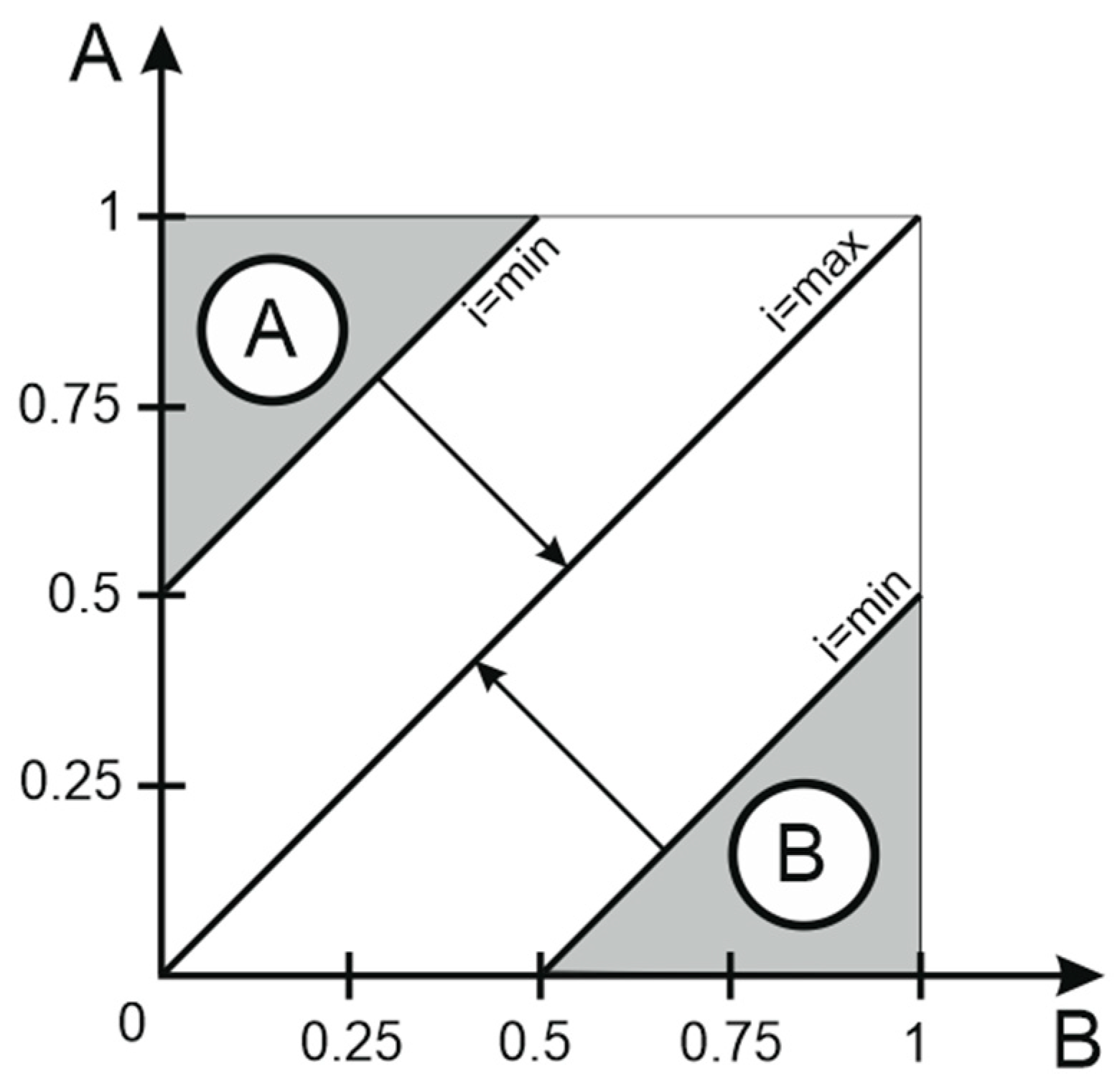
The neutrosophic algorithm has as input the certainty probabilities (truth) provided by the observers on the system’s states. These probabilities are then processed using the described rules in Figure 3. If the difference between the certainties probabilities used at a certain point by the processing algorithm is larger than a certain threshold found by trial and error, then we will consider that the uncertainty percentage between the compared states is null, and the probability that one of the states is true increases. In the case where this difference is not a set threshold, we compute the uncertainty probability by using the formula
where , and “const” depends of the chosen threshold. While the point determined by the two probabilities approaches the main diagonal, the uncertainty approaches the maximum probability value.
From the hyper power set , we can determine the belief masses only for the values (information obtained after observer’s data interpretation) presented below, because the intersection operation represents contradiction in DSm theory and we cannot compute the contradiction values for a single observer using
The neutrosophic probabilities are detailed in Table 2.
5.2. Information Fusion
Having known the trust values of the hyper power set elements , presented in Table 2, we apply the fusion algorithm, using the classic DSm combination rule, detailed in Section 4.2.3.
Appling Equation (4), we get the following formulas for the combination values:
During the fusion process, between the information provided by the two observers contradiction situations may appear. These are included in the hyper power set and are described in Table 3.
Fusion values for contradiction are determined as
5.3. Data Deneutrosophication and Decision-Making
The combination values found in the previous section are deneutrosophicated using the logic diagram presented in Figure 4. For the decision-making algorithm we opted to use Petri nets [64], for it is easier to notice the system’s states transitions. The decision-making diagram proved to have a certain difficulty level, which required adding three sub diagrams:
- sub_p1 (Figure 5)—this sub diagram deals with the contradiction between:
- the certainty that the target object is a ‘sphere’ and the uncertainty that the target object is either a ‘parallelepiped’ or a ‘cylinder’.
- the certainty that the target object is a ‘parallelepiped’ and the uncertainty that the target object is either a ‘sphere’ or a ‘cylinder’.
- the certainty that the target object is a ‘cylinder’ and the uncertainty that the target object is either a ‘parallelepiped’ or a ‘sphere’.
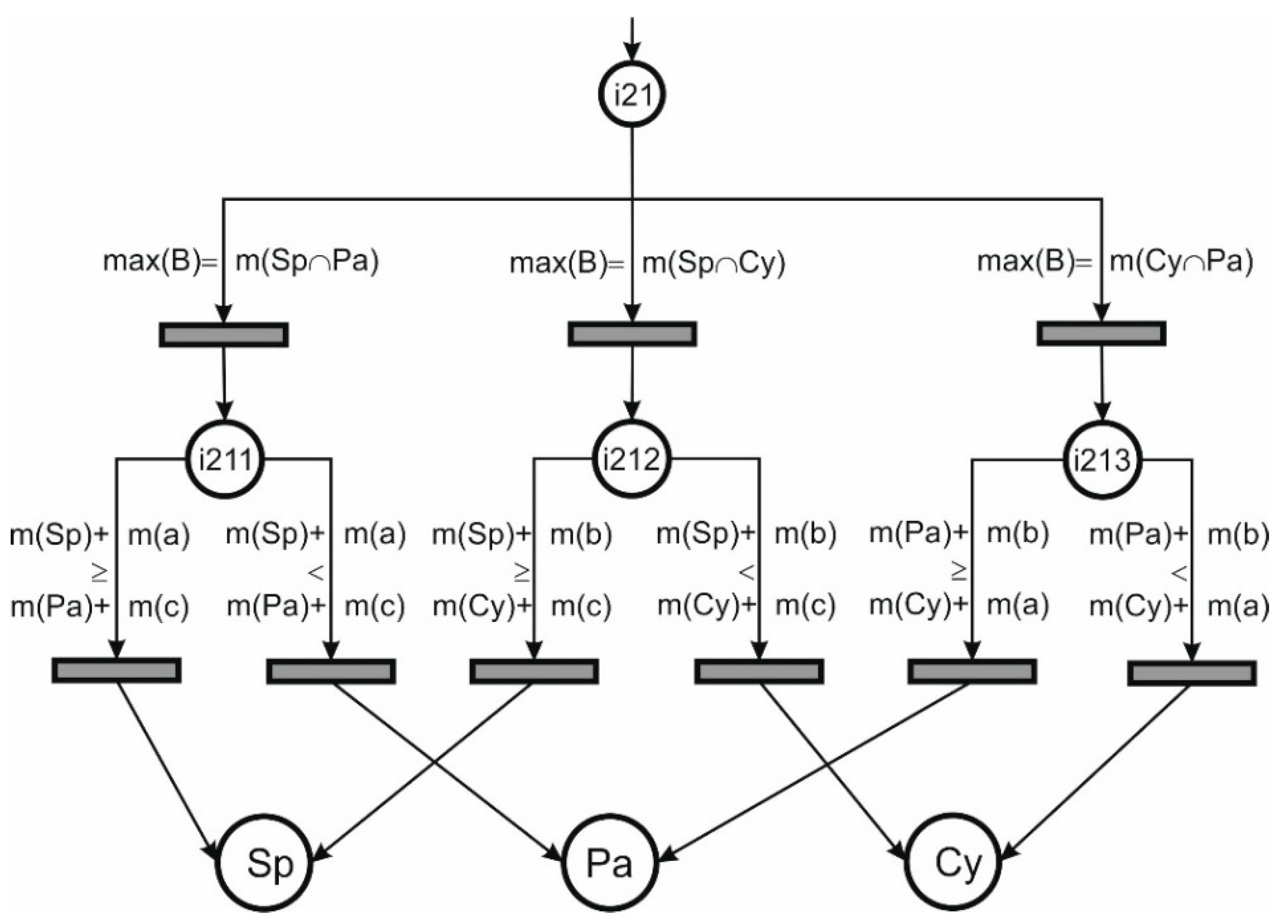
- sub_p2 (Figure 6)—this sub diagram deals with the contradiction between:
- The certainty that the target object is a ‘sphere’ and a ‘parallelepiped’.
- The certainty that the target object is a ‘sphere’ and a ‘cylinder’.
- The certainty that the target object is a ‘cylinder’ and a ‘parallelepiped’.
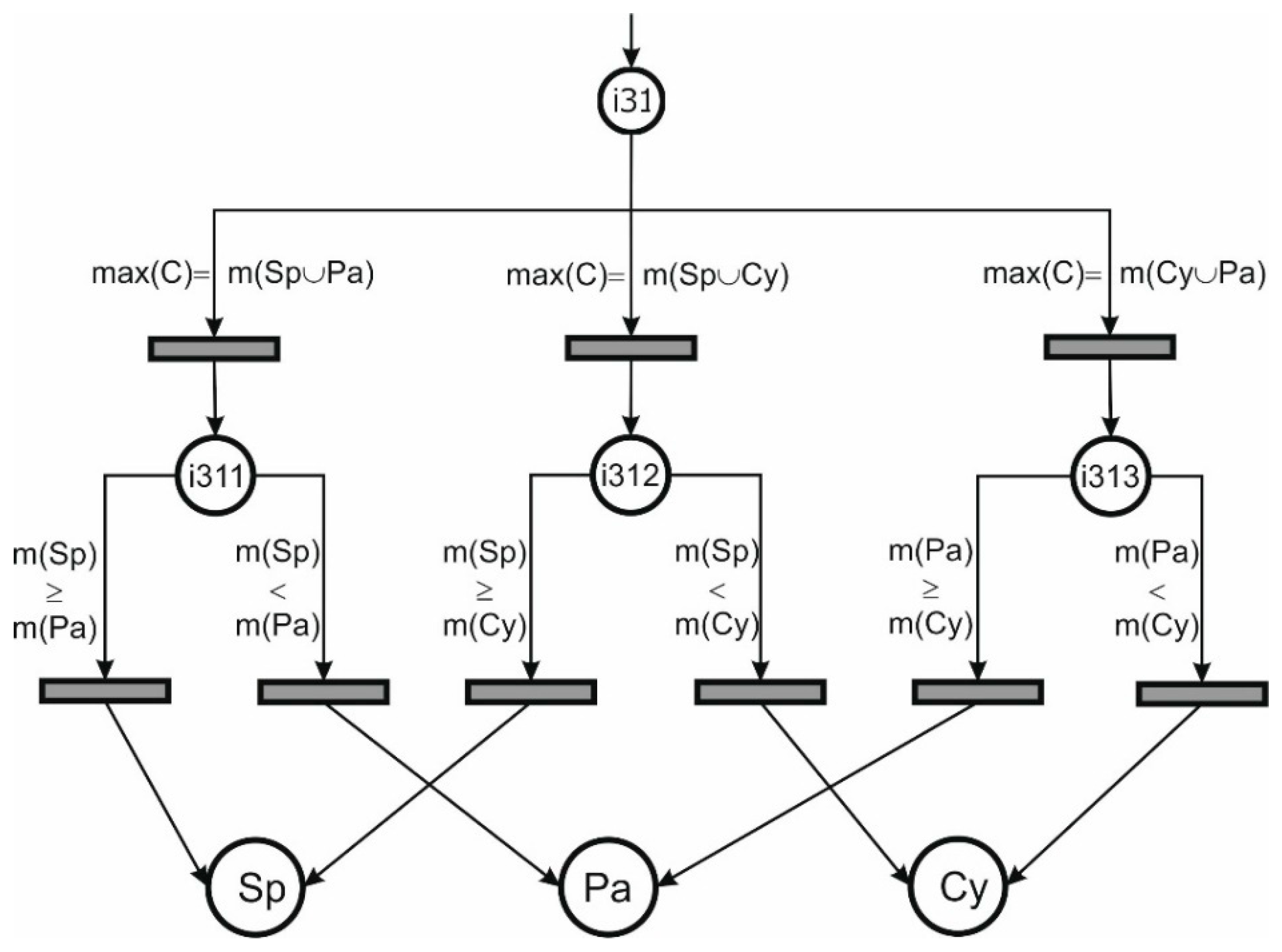
- sub_p3 (Figure 7)—this sub diagram deals with the uncertainty that the target object is:
- a ‘sphere’ or a ‘parallelepiped’
- a ‘sphere’ or a ‘cylinder’
- a ‘cylinder’ or a ‘parallelepiped’
With the help of the Petri diagram (Figure 4), we take the decision of sorting the target object in one of the three categories, as follows:
- Determine .
- If , the contradiction between the certainty value that the target object is a ‘sphere’ and the uncertainty value that the target object is a ‘cylinder’ or ‘parallelepiped’ is compared with a threshold determined through an experimental trial-error process. If this is higher than or equal to the chosen threshold, the target object is a ‘sphere’.
- If , the contradiction between the certainty value that the target object is ‘parallelepiped’ and the uncertainty value that the target object is a ‘sphere’ or ‘cylinder’ is compared with the threshold mentioned above. If this is higher than or equal to the chosen threshold, the target object is a ‘parallelepiped’.
- If , the contradiction between the certainty value that the target object is a ‘cylinder’ and the uncertainty value that the target object is a ‘parallelepiped’ or ‘sphere’ is compared with the threshold mentioned above. If this is higher than or equal to the chosen threshold, the target object is a ‘cylinder’.
If none of the three conditions are met, we proceed to the next step: - Determine
- If , the contradiction between the certainty values that the target object is a ‘sphere’ and ‘parallelepiped’ is compared with a threshold determined through an experimental trial-error process. If this is higher or equal with the chosen threshold, we check if . If this condition if fulfilled, then the target objects is a ‘sphere’. Otherwise, the target object is ‘parallelepiped’.
- If , the contradiction between the certainty values that the target object is a ‘sphere’ and ‘cylinder’ is compared with the threshold mentioned above. If this is higher or equal with the chosen threshold, we check if . If this condition if fulfilled, then the target objects is a ‘sphere’. Otherwise, the target object is a ‘cylinder’.
- If , the contradiction between the certainty values that the target object is a ‘cylinder’ and a ‘parallelepiped’ is compared with the threshold mentioned above. If this is higher or equal with the chosen threshold, we check if . If this condition if fulfilled, then the target objects is a ‘cylinder’. Otherwise, the target object is a ‘parallelepiped’.
If in none of the situations, the contradiction is not larger that the chosen threshold, we go to the next step: - Determine
- If , the uncertainty probability that the target object is a ‘sphere’ or ‘ parallelepiped’ is larger than a threshold determined through an experimental trial-error process, we check if . If the condition is fulfilled, the target object is a ‘sphere’. Otherwise, the target object is a ‘parallelepiped’.
- If , the uncertainty probability that the target object is a ‘sphere’ or ‘cylinder’ is larger than the threshold mentioned above, we check if . If the condition is fulfilled, the target object is a ‘sphere’. Otherwise, the target object is a ‘cylinder’.
- If , the uncertainty probability that the target object is a ‘cylinder’ or ‘ parallelepiped’ is larger than the threshold mentioned above, we check if . If the condition is fulfilled, the target object is a ‘cylinder’. Otherwise, the target object is a ‘parallelepiped’.
If none of the hypotheses mentioned above are not fulfilled, we go to the next step: - Determine
- If , the target object is a ‘sphere’.
- If , the target object is a ‘parallelepiped’.
- If , the target object is a ‘cylinder’.
6. Discussion
As mentioned in the introduction chapter, the main goal of this paper is to find a way to grasp objects according to their shape. This is done by classifying the target objects into three main classes: sphere, parallelepiped, and cylinder.
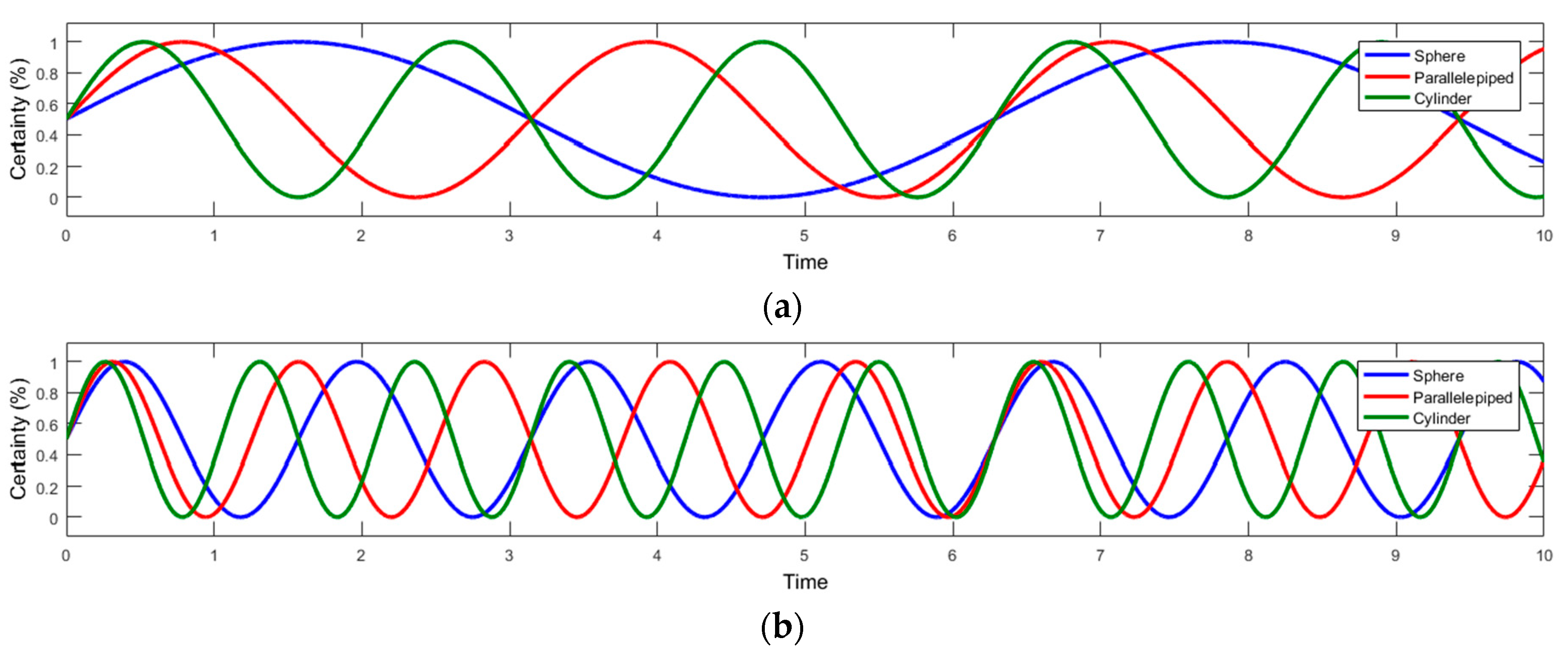
To determine the shape of the target objects, the robot work environment was scanned with a stereovision system and a Kinect sensor, with the purpose of creating a 3D image of the surrounding space in which the robot must fulfill its task. From the two created images, the target object is selected and then it is compared with three templates, which represent a sphere, a cube, and a cylinder. With a template matching algorithm the matching percentage is determined for each of the templates. These percentages (Figure 8), represents the data gathered from the observers, for the fusion problem. Because we wanted to test and verify the decision-making algorithm for as many cases as possible, the observers’ values were simulated using sine signals with different frequency and amplitude of 1 (Figure 8). This amplitude represents the maximum probability percentage that a certain type of object is found by the template matching algorithm.
On these input data, we then apply a neutrosophication algorithm with the purpose of obtaining the generalized belief assignment values for each of the statements an observer is doing:
- The certainty probability that the object is a ‘sphere’ (Figure 9a,h)
- The certainty probability that the object is a ‘parallelepiped’ (Figure 9b,i)
- The certainty probability that the object is a ‘cylinder’ (Figure 9c,j)
- The uncertainty probability that the object is a ‘sphere’ or a ‘parallelepiped’ (Figure 9d,k)
- The uncertainty probability that the object is a ‘sphere’ or a ‘cylinder’ (Figure 9e,l)
- The uncertainty probability that the object is a ‘cylinder’ or a ‘parallelepiped’ (Figure 9f,m)
- The uncertainty probability that the object is a ‘sphere’, a ‘cylinder’, or a ‘parallelepiped’ (Figure 9g,n).
After the belief values were computed for each statements of the observers, we go to the data fusion step (Figure 10).
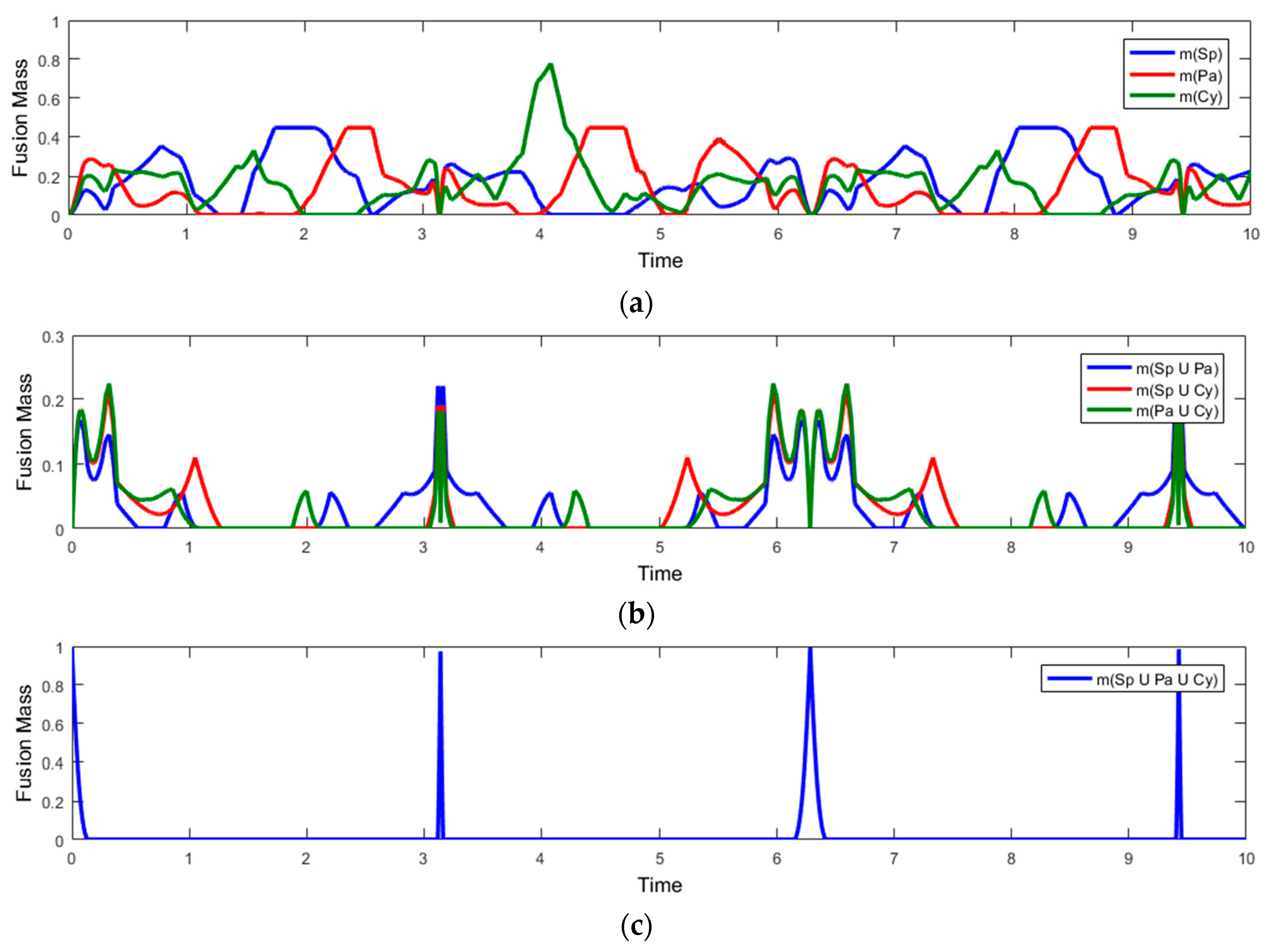
With the help of belief values presented in Figure 10 and computed using the neutrosophication method presented in Section 5.1 and Section 5.2, we find the fusion values, presented in Figure 11.
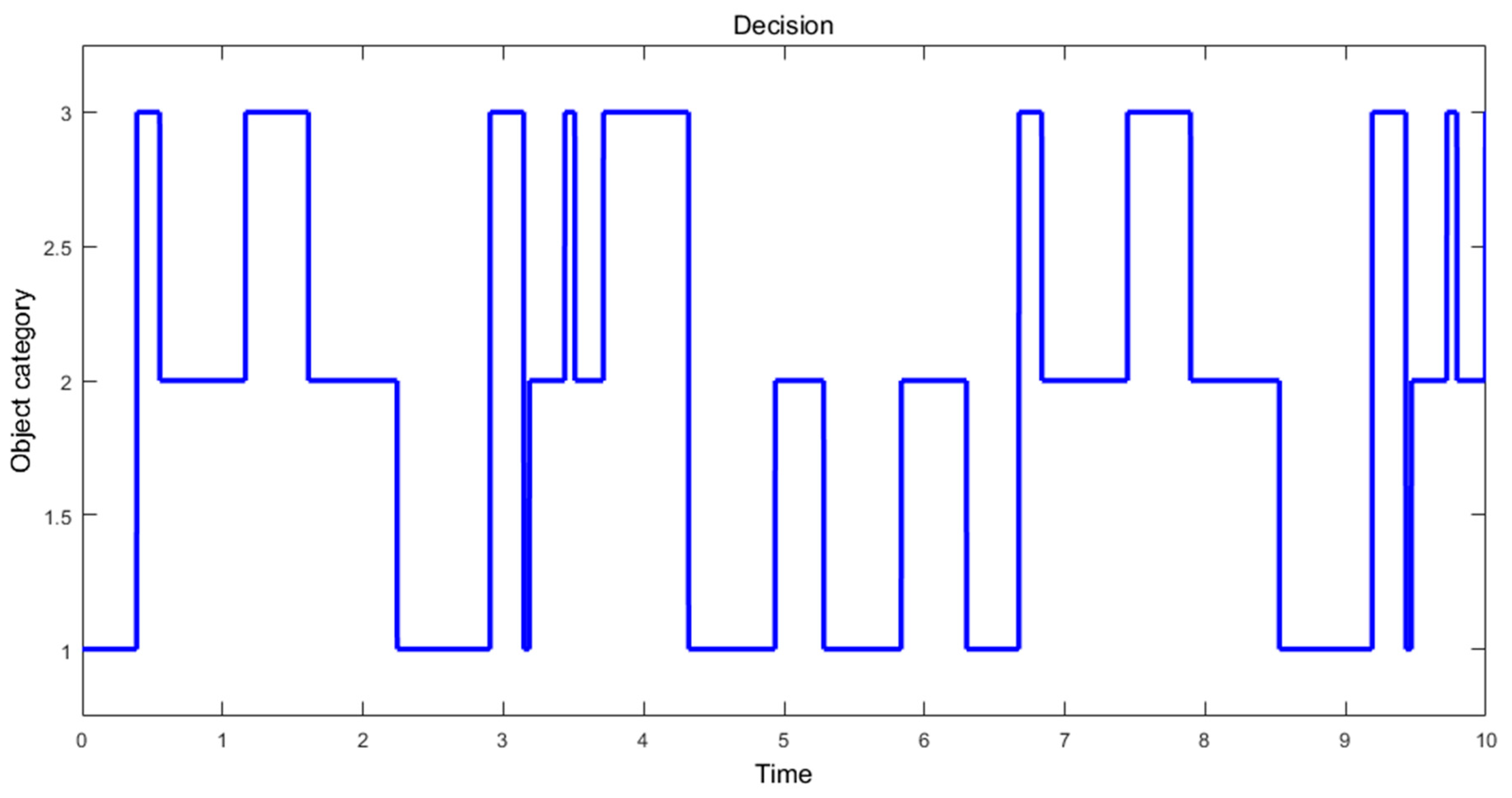
Using the fusion values and the decision-making diagram (Figure 4), from Section 5.2, we can sort the desired object into the three categories: sphere, parallelepiped, and cylinder. The obtained results are presented in Figure 12.
As one can see in Figure 11, the fusion values for certainty, uncertainty and contradiction are minimum. The only exception is the fusion value for the uncertainty that the target object is “sphere” or “parallelepiped” or “cylinder”, , when the data received from the observers are identical and not contradicting, the uncertainty is maximum. This means
Therefore, the system cannot decide on a single state. This is why the robotic hand will maintain its starting position until the system will decide the target object’s category. This indecision period of time takes about 0.07 s. When the sensor values about the target object are changed from the equal values presented above, the algorithm is able to provide a solution.
The indecision also reaches high values at the time 3.14s, 6.28s, and 9.42s of the simulation, in the conditions that the observer’s statements are close in value with the already presented case from above
for the moment s
for the moment s and
for the moment s.
In Table 4, we present the general belief assignment values, the fusion values and the decision made by the algorithm for the situations previously mentioned.
In all three cases, the uncertainty is quite large, and the algorithm ask for restarting the decision process and keeps the decision taken in previous decision process. In our case the decision was that the object is a ‘cylinder’, ‘sphere’, and ‘cylinder’ for the three analyzed points.
Analyzing Figure 11a, at the time of 4.08 s the object is decided to be a ‘cylinder’ because the probability that the target object is a cylinder is very high, .
For the time interval of 4.3–4.9 s, where in Figure 11d the contradiction between the target object being a ‘sphere’ or a ‘parallelepiped’ is larger than that the target object is a ‘sphere’ or a ‘cylinder’ respectively a ‘cylinder’ or a ‘parallelepiped’, the object is decided to be a ‘parallelepiped’ at first because the probability for it being a ‘parallelepiped’ is larger than the probability of it being a ‘sphere’ or a ‘cylinder’. This situation is changed starting with second 5 of the simulation, when the probability that the target object is a ‘sphere’ increase, the probability that the same object is a ‘cylinder’ remains low and the probability that the target object is a ‘parallelepiped’ decrease below the value of the ‘sphere’ probability.
7. Conclusions
Any robot, no mater of its purpose, has a task to fulfill. That task can be either of grasping and manipulation or just a transport task. To successfully complete its task, the robot must be equipped with a number of sensors that will provide enough information about the work environment in which the work is being done.
In this paper, we studied the situation in which the robot is equipped with a stereovision system and a Kinect sensor to detect the environment. The robot’s job was to grab and manipulate certain objects. With the help of two different systems, two 3D images of the environment can be created, each one for the two sensor type. In these images, we isolated the target object and it is compared with three template images, obtained through similar methods as the environment images. The three template images represent the 3D virtual model of a sphere, a parallelepiped, and a cylinder. The comparison is achieved with a template matching method, and following that we obtain a matching percentage for each template tested against the desired image.
Because we wanted to develop the decision-making algorithm based on information received from certain template matching methods, we considered as known the information that these algorithms can provide. Moreover, to test different cases, we selected several sine signals that can provide all the different cases that can occur in practice as input for our decision-making algorithm and output for the template matching methods.
The goal of this paper is in part a data fusion problem with the purpose of classifying the objects in visual range of a humanoid robot, so it can fulfill his grasping and manipulation task. We also wanted to label the target object in one of three categories mentioned above, so that during the approach phase on the target object, the robotic hand can prepare for grasping the object, lowering the time needed to complete the task.
The stereovision system and the Kinect sensor presented in Section 3, represent the information sources, called in this paper, the observers, name taken from the neutrosophic logic. These observers specify the state in which the system is. One observer can specify seven states for the searched object.
With the help of neutrosophic logic, we determine the generalized belief values for each of the seven states. The neutrosophic algorithm is applied to information gathered from both of the sensors. We have chosen the neutrosophic logic, because it extends fuzzy logic, providing instruments for also approaching the uncertain situations besides the true and false ones.
Using these belief values, we compute the fusion values on which we apply the classic DSm combination rule, and build the decision-making algorithm presented in Section 5. To help develop this decision-making algorithm we used a Petri net which provided us a clear method of switching through system states under certain conditions.
The decision-making algorithm analyzes the probability of completing all the possible tasks that may appear in sensor data fusion and tackles these possibilities so that for every input the system will have an output.
The presented method can be used successfully in real time applications, because it provides a decision in all the cases in a very short time (Table 5). The algorithm can be extended so that it can use information received from multiple sources or provide a decision starting from a high number of system states. The number of observer/data sources is not limited nor is the system’s states. However, while increasing the number of observers and system’s states, the data to be processed is increased and the decision-making algorithm design is becoming a highly difficult task to achieve.
In the case of autonomous robots, these must be taught what to do and how to complete their tasks. From this, the necessity of developing new intelligent and reasoning system arises. The developed algorithm in this paper can be used successfully for target identification applications, object sorting, image labeling, motion tracking, obstacle avoidance, edge detection, etc.
Author Contributions
Conceptualization, I.-A.G., D.B., and L.V.; Data curation, I.-A.G.; Formal analysis, I.-A.G.; Funding acquisition, L.V.; Investigation, I.-A.G., D.B., and L.V.; Methodology, L.V.; Resources, I.-A.G.; Software, I.-A.G.; Supervision, L.V.; Validation, I.-A.G., D.B., and L.V.; Visualization, I.-A.G., D.B., and L.V.; Writing—original draft, I.-A.G.; Writing—review and editing, L.V.
Funding
The paper was funded by the European Commission Marie Skłodowska-Curie SMOOTH project, Smart Robots for Fire-Fighting, H2020-MSCA-RISE-2016-734875, Yanshan University: “Joint Laboratory of Intelligent Rehabilitation Robot” project, KY201501009, Collaborative research agreement between Yanshan University, China and Romanian Academy by IMSAR, RO, and the UEFISCDI Multi-MonD2 Project, Multi-Agent Intelligent Systems Platform for Water Quality Monitoring on the Romanian Danube and Danube Delta, PCCDI 33/2018, PN-III-P1-1.2-PCCDI2017-2017-0637.
Acknowledgments
This work was developed with the support of the Institute of Solid Mechanics of the Romanian Academy, the European Commission Marie Skłodowska-Curie SMOOTH project, Smart Robots for Fire-Fighting, H2020-MSCA-RISE-2016-734875, Yanshan University: “Joint Laboratory of Intelligent Rehabilitation Robot” project, KY201501009, Collaborative research agreement between Yanshan University, China and Romanian Academy by IMSAR, RO, and the UEFISCDI Multi-MonD2 Project, Multi-Agent Intelligent Systems Platform for Water Quality Monitoring on the Romanian Danube and Danube Delta, PCCDI 33/2018, PN-III-P1-1.2-PCCDI2017-2017-0637.
Conflicts of Interest
The authors declare no conflict of interest.
References
- Vladareanu, V.; Sandru, O.I.; Vladareanu, L.; Yu, H. Extension dynamical stability control strategy for the walking Robots. Int. J. Technol. Manag. 2013, 12, 1741–5276. [Google Scholar]
- Xu, Z.; Kumar, V.; Todorov, E. A low-cost and modular, 20-DOF anthropomorphic robotic hand: Design, actuation and modeling. In Proceedings of the IEEE-RAS International Conference on Humanoid Robots (Humanoids), Atlanta, GA, USA, 15–17 October 2013. [Google Scholar]
- Jaffar, A.; Bahari, M.S.; Low, C.Y.; Jaafar, R. Design and control of a Multifingered anthropomorphic Robotic hand international. Int. J. Mech. Mechatron. Eng. 2011, 11, 26–33. [Google Scholar]
- Roa, M.A.; Argus, M.J.; Leidner, D.; Borst, C.; Hirzinger, G. Power grasp planning for anthropomorphic robot hands. In Proceedings of the 2012 IEEE International Conference on Robotics and Automation (ICRA), Saint Paul, MN, USA, 14–18 May 2012; pp. 563–569. [Google Scholar] [CrossRef]
- Lippiello, V.; Siciliano, B.; Villani, L. Multi-fingered grasp synthesis based on the object Dynamic properties. Robot. Auton. Syst. 2013, 61, 626–636. [Google Scholar] [CrossRef]
- Bullock, I.M.; Ma, R.R.; Dollar, A.M. A hand-centric classification of Human and Robot dexterous manipulation. IEEE Trans. Haptics 2013, 6, 129–144. [Google Scholar] [CrossRef] [PubMed]
- Ormaechea, R.C. Robotic Hands. Adv. Mech. Robot. Syst. 2011, 1, 19–39. [Google Scholar] [CrossRef]
- Enabling the Future. Available online: http://enablingthefuture.org (accessed on 26 March 2018).
- Prattichizzo, D.; Trinkle, J.C. Grasping. In Springer Handbook of Robotics; Siciliano, B., Khatib, O., Eds.; Springer: Berlin, Germany, 2016; pp. 955–988. ISBN 978-3-319-32552-1. [Google Scholar]
- Feix, T.; Romero, J.; Schmiedmayer, H.B.; Dollar, A.M.; Kragic, D. The GRASP taxonomy of human grasp types. IEEE Trans. Hum.-Mach. Syst. 2016, 46, 66–77. [Google Scholar] [CrossRef]
- Alvarez, A.G.; Roby-Brami, A.; Robertson, J.; Roche, N. Functional classification of grasp strategies used by hemiplegic patients. PLoS ONE 2017, 12, e0187608. [Google Scholar] [CrossRef]
- Fermuller, C.; Wang, F.; Yang, Y.Z.; Zampogiannis, K.; Zhang, Y.; Barranco, F.; Pfeiffer, M. Prediction of manipulation actions. Int. J. Comput. Vis. 2018, 126, 358–374. [Google Scholar] [CrossRef]
- Tsai, J.R.; Lin, PC. A low-computation object grasping method by using primitive shapes and in-hand proximity sensing. In Proceedings of the IEEE ASME International Conference on Advanced Intelligent Mechatronics, Munich, Germany, 3–7 July 2017; pp. 497–502. [Google Scholar]
- Song, P.; Fu, Z.Q.; Liu, LG. Grasp planning via hand-object geometric fitting. Vis. Comput. 2018, 34, 257–270. [Google Scholar] [CrossRef]
- Ma, C.; Qiao, H.; Li, R.; Li, X.Q. Flexible robotic grasping strategy with constrained region in environment. Int. J. Autom. Comput. 2017, 14, 552–563. [Google Scholar] [CrossRef] [Green Version]
- Stavenuiter, R.A.J.; Birglen, L.; Herder, J.L. A planar underactuated grasper with adjustable compliance. Mech. Mach. Theory 2017, 112, 295–306. [Google Scholar] [CrossRef]
- Choi, C.; Yoon, S.H.; Chen, C.N.; Ramani, K. Robust hand pose estimation during the interaction with an unknown object. In Proceedings of the IEEE International Conference on Computer Vision, Venice, Italy, 22–29 October 2017; pp. 3142–3151. [Google Scholar]
- Seredynski, D.; Szynkiewicz, W. Fast grasp learning for novel objects. In Challenges in Automation, Robotics and Measurement Techniques, Proceedings of AUTOMATION-2016, Warsaw, Poland, 2–4 March 2016; Advances in Intelligent Systems and Computing Book Series; Springer: Warsaw, Poland, 2016; Volume 440, pp. 681–692. ISBN 978-3-319-29357-8; 978-3-319-29356-1. [Google Scholar]
- Shaw-Cortez, W.; Oetomo, D.; Manzie, C.; Choong, P. Tactile-based blind grasping: A discrete-time object manipulation controller for robotic hands. IEEE Robot. Autom. Lett. 2018, 3, 1064–1071. [Google Scholar] [CrossRef]
- Gu, H.W.; Zhang, Y.F.; Fan, S.W.; Jin, M.H.; Liu, H. Grasp configurations optimization of dexterous robotic hand based on haptic exploration information. Int. J. Hum. Robot. 2017, 14. [Google Scholar] [CrossRef]
- Yamakawa, Y.; Namiki, A.; Ishikawa, M.; Shimojo, M. Planning of knotting based on manipulation skills with consideration of robot mechanism/motion and its realization by a robot hand system. Symmetry 2017, 9, 194. [Google Scholar] [CrossRef]
- Nacy, S.M.; Tawfik, M.A.; Baqer, I.A. A novel approach to control the robotic hand grasping process by using an artificial neural network algorithm. J. Intell. Syst. 2017, 26, 215–231. [Google Scholar] [CrossRef]
- Zaidi, L.; Corrales, J.A.; Bouzgarrou, B.C.; Mezouar, Y.; Sabourin, L. Model-based strategy for grasping 3D deformable objects using a multi-fingered robotic hand. Robot. Auton. Syst. 2017, 95, 196–206. [Google Scholar] [CrossRef]
- Liu, H.; Meusel, P.; Hirzinger, G.; Jin, M.; Liu, Y.; Xie, Z. The modular multisensory DLR-HIT-Hand: Hardware and software architecture. IEEE/ASME Trans. Mechatron. 2008, 13, 461–469. [Google Scholar] [CrossRef]
- Zollo, L.; Roccella, S.; Guglielmelli, E.; Carrozza, M.C.; Dario, P. Biomechatronic design and control of an anthropomorphic artificial hand for prosthetic and robotic applications. IEEE/ASME Trans. Mechatron. 2007, 12, 418–429. [Google Scholar] [CrossRef]
- Lopez-Damian, E.; Sidobre, D.; Alami, R. Grasp planning for non-convex objects. Int. Symp. Robot. 2009, 36. [Google Scholar] [CrossRef]
- Miller, A.T.; Knoop, S.; Christensen, H.I.; Allen, P.K. Automatic grasp planning using shape primitives. In Proceedings of the 2003 IEEE International Conference on Robotics and Automation (Cat. No.03CH37422), Taipei, Taiwan, 14–19 September 2003. [Google Scholar]
- Napier, J. The prehensile movements of the human hand. J. Bone Jt. Surg. 1956, 38, 902–913. [Google Scholar] [CrossRef]
- Cutkosky, M.R.; Wright, P.K. Modeling manufacturing grips and correlation with the design of robotic hands. In Proceedings of the 1986 IEEE International Conference on Robotics and Automation, San Francisco, CA, USA, 7–10 April 1986; pp. 1533–1539. [Google Scholar]
- Iberall, T. Human prehension and dexterous robot hands. Int. J. Robot. Res. 1997, 16, 285–299. [Google Scholar] [CrossRef]
- Stansfield, S.A. Robotic grasping of unknown objects: A knowledge-based approach. Int. J. Robot. Res. 1991, 10, 314–326. [Google Scholar] [CrossRef]
- Lai, X.; Wang, H.; Xu, Y. A real-time range finding system with binocular stereo vision. Int. J. Adv. Robot. Syst. 2012, 9, 26. [Google Scholar] [CrossRef]
- Oliver, A.; Wünsche, B.C.; Kang, S.; MacDonald, B. Using the Kinect as a navigation sensor for mobile robotics. In Proceedings of the 27th Conference on Image and Vision Computing New Zealand, Dunedin, New Zealand, 26–28 November 2012; pp. 509–514, ISBN 978-1-4503-1473-2. [Google Scholar]
- Aljarrah, I.A.; Ghorab, A.S.; Khater, I.M. Object recognition system using template matching based on signature and principal component analysis. Int. J. Digit. Inf. Wirel. Commun. 2012, 2, 156–163. [Google Scholar]
- Smarandache, F.; Dezert, J. Applications and Advances of DSmT for Information Fusion; American Research Press: Rehoboth, DE, USA, 2009; Volume 3. [Google Scholar]
- Khaleghi, B.; Khamis, A.; Karray, F.; Razavi, S.N. Multisensor data fusion: A review of the state-of-the-art. Inf. Fusion 2013, 14, 28–44. [Google Scholar] [CrossRef]
- Jian, Z.; Hongbing, C.; Jie, S.; Haitao, L. Data fusion for magnetic sensor based on fuzzy logic theory. In Proceedings of the IEEE International Conference on Intelligent Computation Technology and Automation, Shenzhen, China, 28–29 March 2011. [Google Scholar]
- Munz, M.; Dietmayer, K.; Mahlisch, M. Generalized fusion of heterogeneous sensor measurements for multi target tracking. In Proceedings of the 13th Conference on Information Fusion (FUSION), Edinburgh, UK, 26–29 July 2010; pp. 1–8. [Google Scholar]
- Jiang, Y.; Wang, H.G.; Xi, N. Target object identification and location based on multi-sensor fusion. Int. J. Autom. Smart Technol. 2013, 3, 57–67. [Google Scholar] [CrossRef]
- Hall, D.L.; Hellar, B.; McNeese, M.D. Rethinking the data overload problem: Closing the gap between situation assessment and decision-making. In Proceedings of the National Symposium on Sensor Data Fusion, McLean, VA, USA, 11–15 June 2007. [Google Scholar]
- Esteban, J.; Starr, A.; Willetts, R.; Hannah, P.; Bryanston-Cross, P. A review of data fusion models and architectures: Towards engineering guidelines. Neural Comput. Appl. 2005, 14, 273–281. [Google Scholar] [CrossRef] [Green Version]
- Chilian, A.; Hirschmuller, H.; Gorner, M. Multisensor data fusion for robust pose estimation of a six-legged walking robot. In Proceedings of the 2011 IEEE/RSJ International Conference on Intelligent Robots and Systems (IROS), San Francisco, CA, USA, 25–30 September 2011. [Google Scholar]
- Dasarathy, B.V. Editorial: Information fusion in the realm of medical applications—A bibliographic glimpse at its growing appeal. Inf. Fusion 2012, 13, 1–9. [Google Scholar] [CrossRef]
- Hall, D.L.; Linn, R.J. Survey of commercial software for multisensor data fusion. Proc. SPIE 1993. [Google Scholar] [CrossRef]
- Vladareanu, L.; Vladareanu, V.; Schiopu, P. Hybrid force-position dynamic control of the robots using fuzzy applications. Appl. Mech. Mater. 2013, 245, 15–23. [Google Scholar] [CrossRef]
- Gaines, B.R. Fuzzy and probability uncertainty logics. Inf. Control 1978, 38, 154–169. [Google Scholar] [CrossRef]
- Shafer, G. A Mathematical Theory of Evidence; Princeton University Press: Princeton, NJ, USA, 1976; Volume 73. [Google Scholar]
- Sahbani, A.; El-Khoury, S.; Bidaud, P. An overview of 3D object grasp synthesis algorithms. Robot. Auton. Syst. 2012, 60, 326–336. [Google Scholar] [CrossRef] [Green Version]
- De Souza, R.; El Khoury, S.; Billard, A. Towards comprehensive capture of human grasping and manipulation skills. In Proceedings of the Thirteenth International Symposium on the 3-D Analysis of Human Movement, Lausanne, Switzerland, 14–17 July 2014. [Google Scholar]
- Bullock, I.M.; Dollar, A.M. Classifying human manipulation behavior. In Proceedings of the 2011 IEEE International Conference on Rehabilitation Robotics, Zurich, Switzerland, 29 June–1 July 2011; pp. 1–6. [Google Scholar]
- Morales, A.; Azad, P.; Asfour, T.; Kraft, D.; Knoop, S.; Dillmann, R.; Kargov, A.; Pylatiuk, C.H.; Schulz, S. An anthropomorphic grasping approach for an assistant humanoid robot. Int. Symp. Robot. 2006, 1956, 149. [Google Scholar]
- Etienne–Cwnmings, R.; Pouliquen, P.; Lewis, M. A Single chip for imaging, color segmentation, histogramming and template matching. Electron. Lett. 2002, 2, 172–174. [Google Scholar] [CrossRef]
- Guskov, I. Kernel—based template alignment. In Proceedings of the 2006 IEEE Computer Society Conference on Computer Vision and Pattern Recognition (CVPR’06), New York, NY, USA, 17–22 June 2006; pp. 610–617. [Google Scholar]
- Smarandache, F.; Dezert, J. Applications and Advances of DSmT for Information Fusion; American Research Press: Rehoboth, DE, USA, 2004. [Google Scholar]
- Smarandache, F.; Vladareanu, L. Applications of neutrosophic logic to robotics: An introduction. In Proceedings of the 2011 IEEE International Conference on Granular Computing, Kaohsiung, Taiwan, 8–10 November 2011; pp. 607–612. [Google Scholar]
- Gal, I.A.; Vladareanu, L.; Yu, H. Applications of neutrosophic logic approaches in ‘RABOT’ real time control. In Proceedings of the SISOM 2012 and Session of the Commission of Acoustics, Bucharest, Romania, 30–31 May 2013. [Google Scholar]
- Gal, I.A.; Vladareanu, L.; Munteanu, R.I. Sliding motion control with bond graph modeling applied on a robot leg. Rev. Roum. Sci. Tech. 2010, 60, 215–224. [Google Scholar]
- Vladareanu, V.; Dumitrache, I.; Vladareanu, L.; Sacala, I.S.; Tont, G.; Moisescu, M.A. Versatile intelligent portable robot control platform based on cyber physical systems principles. Stud. Inform. Control 2015, 24, 409–418. [Google Scholar] [CrossRef]
- Melinte, D.O.; Vladareanu, L.; Munteanu, R.A.; Wang, H.; Smarandache, F.; Ali, M. Nao robot in virtual environment applied on VIPRO platform. In Proceedings of the Annual Symposium of the Institute of Solid Mechanics and Session of the Commission of Acoustics, Bucharest, Romania, 21–22 May 2016; Volume 57. [Google Scholar]
- Smarandache, F. A unifying field in logics: Neutrosophic field. Multiple-valued logic. Int. J. 2002, 8, 385–438. [Google Scholar]
- Wang, H.; Smarandache, F.; Zhang, Y.Q.; Sunderraman, R. Interval Neutrosophic Sets and Logic: Theory and Application in Computing; HEXIS Neutrosophic Book Series No.5; Georgia State University: Atlanta, GA, USA, 2005; ISBN 1-931233-94-2. [Google Scholar]
- Smarandache, F. Neutrosophy: Neutrosophic Probability, Set, and Logic: Analytic Synthesis & Synthetic Analysis; American Research Press: Gallup, NM, USA, 1998; 105p, ISBN 1-87958-563-4. [Google Scholar]
- Rosell, J.; Sierra, X.; Palomo, F.L. Finding grasping configurations of a dexterous hand and an industrial robot. In Proceedings of the 2005 IEEE International Conference on Robotics and Automation, Barcelona, Spain, 18–22 April 2005; pp. 1178–1183. [Google Scholar] [CrossRef]
- Emadi, S.; Shams, F. Modeling of component diagrams using Petri Nets. Indian J. Sci. Technol. 2010, 3, 1151–1161. [Google Scholar] [CrossRef]
Figure 1.
Graphical representation of DSm classic rule of combination for [35].
Figure 1.
Graphical representation of DSm classic rule of combination for [35].
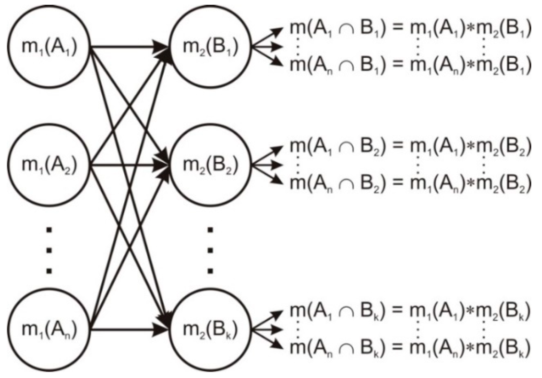
Figure 2.
Diagram of the proposed algorithm.

Figure 3.
Data neutrosophication rule for the observer’s data.

Figure 4.
Petri diagram for decision-making algorithm.

Figure 5.
Petri net for sub_p1.
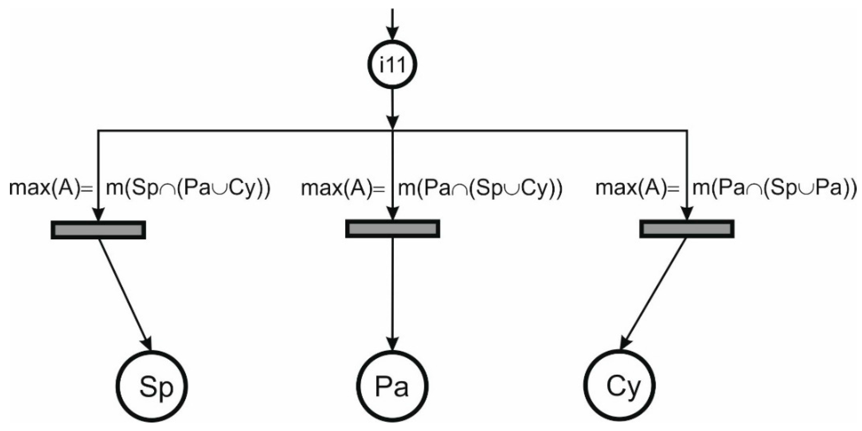
Figure 6.
Petri net for sub_p2.

Figure 7.
Petri net for sub_p3.

Figure 8.
Simulation of the information provided by the two sensors/observers: (a) first observer detection; (b) second observer detection.
Figure 8.
Simulation of the information provided by the two sensors/observers: (a) first observer detection; (b) second observer detection.

Figure 9.
Generalized trust values. From a to g correspond to Observer 1 and from h to n for Observer 2 as follows: (a) ; (b) ; (c) ; (d) ; (e) ; (f) ; (g) ; (h) ; (i) ; (j) ; (k) ; (l) ; (m) ; (n) .
Figure 9.
Generalized trust values. From a to g correspond to Observer 1 and from h to n for Observer 2 as follows: (a) ; (b) ; (c) ; (d) ; (e) ; (f) ; (g) ; (h) ; (i) ; (j) ; (k) ; (l) ; (m) ; (n) .
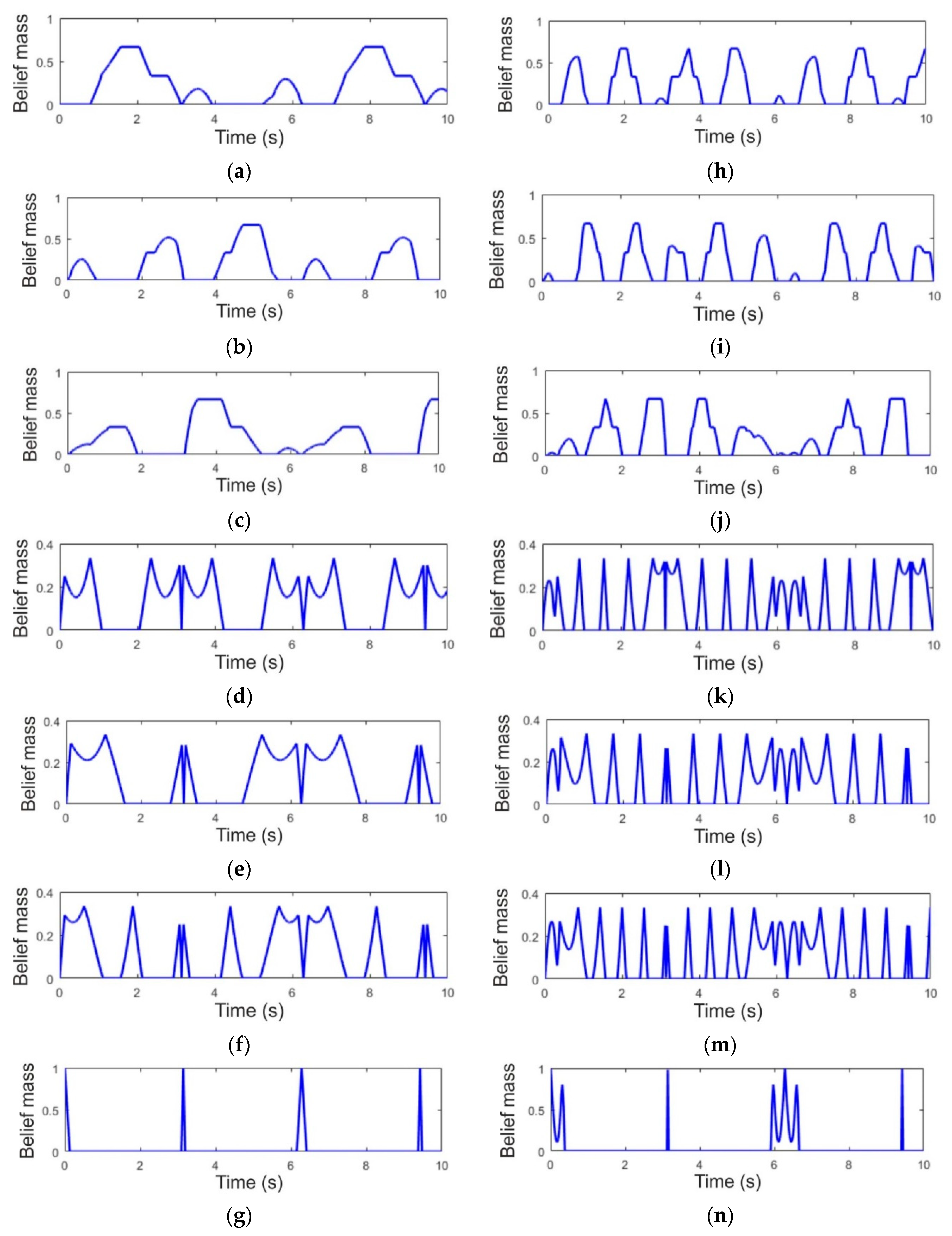
Figure 10.
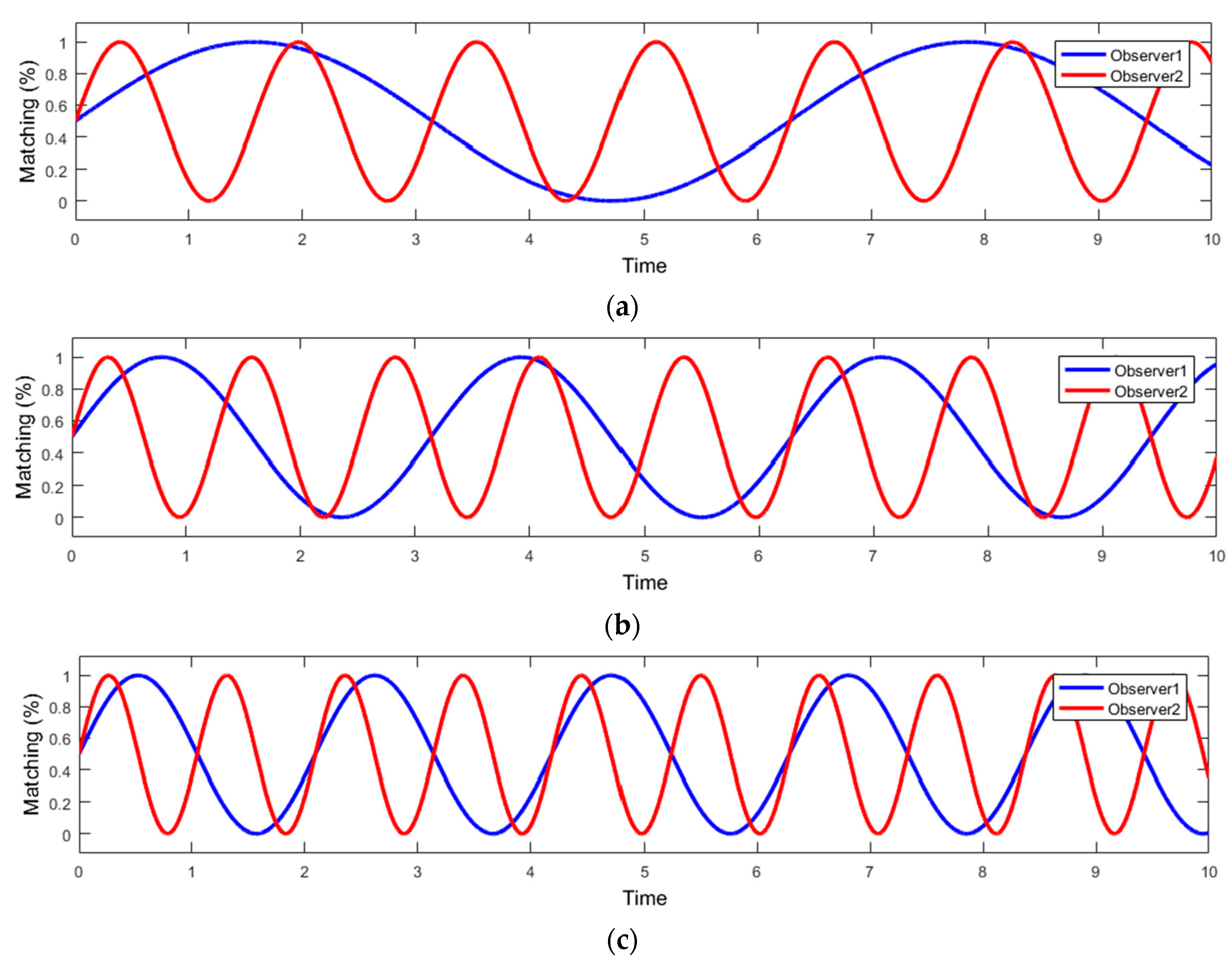
Data fusion: (a) Observer 1 vs. Observer 2 for sphere objects; (b) Observer 1 vs. Observer 2 for parallelepiped objects; (c) Observer 1 vs. Observer 2 for cylinder objects.
Figure 10.
Data fusion: (a) Observer 1 vs. Observer 2 for sphere objects; (b) Observer 1 vs. Observer 2 for parallelepiped objects; (c) Observer 1 vs. Observer 2 for cylinder objects.

Figure 11.
Fusion values: (a) Fusion values of , and ; (b) Fusion values of , , ; (c) Fusion value of ; (d) Fusion values of , , ; (e) Fusion values of , , .
Figure 11.
Fusion values: (a) Fusion values of , and ; (b) Fusion values of , , ; (c) Fusion value of ; (d) Fusion values of , , ; (e) Fusion values of , , .

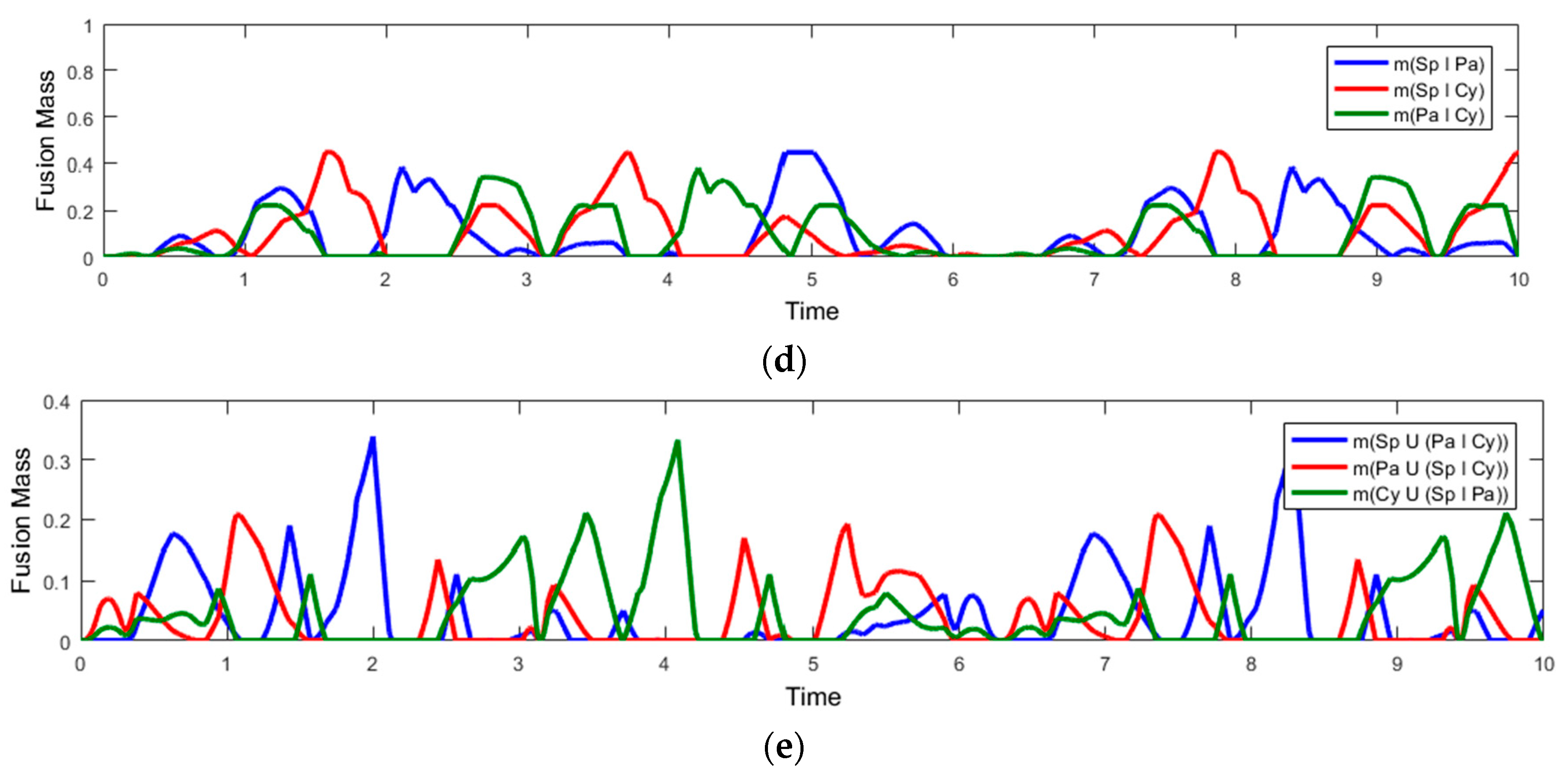
Figure 12.
Object category decision, obtained from the proposed algorithm. Value 1 represents decision for sphere, Value 2 represents decision for parallelepiped, and Value 3 represents decision for cylinder.
Figure 12.
Object category decision, obtained from the proposed algorithm. Value 1 represents decision for sphere, Value 2 represents decision for parallelepiped, and Value 3 represents decision for cylinder.


Table 1.
Grasping position for certain tasks.
| Object | Activity | Grasping Position |
|---|---|---|
| Bottles, cups, and mugs | Transport, pouring/filling | Force: Cylindrical grasping (from the side or the top) |
| Cups (using handles) | Pouring/filling | Force: Lateral grasping Precision: Prismatic grasping |
| Plates/trays | Transport Receiving from humans | Power: Lateral grasping Precision: Prismatic grasping No grasp: pushing (open hand) |
| Pens, cutlery | Transport | Precision: Prismatic grasping |
| Door handle | Open/Close | Force: Cylindrical grasping No grasp: Hook |
| Small objects | Transport | Power: Spherical grasping Precision: Circular grasping (tripod) |
| Switches, buttons | Pushing | No grasp: Button pressing |
| Round switches, bottle caps | Rotation | Force: Lateral grasping Precision: Circular grasping (tripod) |
Table 2.
Grasping position for certain tasks.
| Mathematical Representation | Description |
|---|---|
| Certainty that the target object is a ‘sphere’ | |
| Certainty that the target object is a ‘parallelepiped’ | |
| Certainty that the target object is a ‘cylinder’ | |
| Uncertainty that the target object is a ‘sphere’ or ‘parallelepiped’ | |
| Uncertainty that the target object is a ‘sphere’ or ‘cylinder’ | |
| Uncertainty that the target object is a ‘cylinder’ or ‘parallelepiped’ | |
| Uncertainty that the target object is a ‘sphere’, ‘cylinder’, or ‘parallelepiped’ |
Table 3.
Contradictions that may appear between the neutrosophic probabilities.
| Mathematical Representation | Description |
|---|---|
| Contradiction between the certainties that the target object is a ‘sphere’ and ‘parallelepiped’ | |
| Contradiction between the certainties that the target object is a ‘sphere’ and ‘cylinder’ | |
| Contradiction between the certainties that the target object is a ‘cylinder’ and ‘parallelepiped’ | |
| Contradiction between the certainty that the target object is a ‘sphere’ and the uncertainty that the target object is a ‘cylinder’ or ‘parallelepiped’ | |
| Contradiction between the certainty that the target object is a ‘parallelepiped’ and the uncertainty that the target object is a ‘sphere’ or ‘cylinder’ | |
| Contradiction between the certainty that the target object is ‘cylinder’ and the uncertainty that the target object is a ‘parallelepiped’ or ‘sphere’ | |
| Contradiction between the certainties that the target object is a ‘sphere’, ‘cylinder’, and ‘parallelepiped’ |
Table 4.
Generalized trust values, fusion values, and decisions for the analyzed situations.
| Time | 3.14 s | 6.28 s | 9.42 s | |||||
|---|---|---|---|---|---|---|---|---|
| Source | State | Obs. 1 | Obs. 2 | Obs. 1 | Obs. 2 | Obs. 1 | Obs. 2 | |
| Hypothesis | ||||||||
| Generalized belief assignment values | ||||||||
| 0.0001 | 0.0001 | 0.0001 | 0.0001 | 0.0005 | 0.0007 | |||
| 0.0001 | 0 | 0 | 0 | 0.0011 | 0.0067 | |||
| 0 | 0.0008 | 0 | 0 | 0 | 0 | |||
| 0.0106 | 0.0234 | 0.0085 | 0.0085 | 0.0317 | 0.0692 | |||
| 0.0106 | 0.0231 | 0.0085 | 0.0085 | 0.0315 | 0.0669 | |||
| 0.0106 | 0.0231 | 0.0085 | 0.0085 | 0.0312 | 0.0662 | |||
| 0.9680 | 0.9296 | 0.9744 | 0.9744 | 0.9040 | 0.7904 | |||
| Fusion values | ||||||||
| 0.0006 | 0.0001 | 0.0054 | ||||||
| 0.0006 | 0.0003 | 0.0053 | ||||||
| 0.0012 | 0.0002 | 0.0106 | ||||||
| 0.0328 | 0.0166 | 0.0898 | ||||||
| 0.0325 | 0.0166 | 0.0875 | ||||||
| 0.0324 | 0.0166 | 0.0866 | ||||||
| 0.8999 | 0.9495 | 0.7145 | ||||||
| 0 | 0 | 0 | ||||||
| 0 | 0 | 0 | ||||||
| 0 | 0 | 0 | ||||||
| 0 | 0 | 0.0001 | ||||||
| 0 | 0 | 0.0001 | ||||||
| 0 | 0 | 0.0002 | ||||||
| Decision | Cylinder | Sphere | Cylinder | |||||
Table 5.
Average execution time of the presented algorithm.
| Method | Execution Time (s) |
|---|---|
| Data neutrosophication for Obs. 1 | 0.0026 |
| Data neutrosophication for Obs. 2 | 0.0026 |
| Data fusion using DSmT | 0.0002 |
| Data deneutrosophication/decision-making | 0.0092 |
| Total time | 0.0146 |
© 2018 by the authors. Licensee MDPI, Basel, Switzerland. This article is an open access article distributed under the terms and conditions of the Creative Commons Attribution (CC BY) license (http://creativecommons.org/licenses/by/4.0/).
Share and Cite
MDPI and ACS Style
Gal, I.-A.; Bucur, D.; Vladareanu, L. DSmT Decision-Making Algorithms for Finding Grasping Configurations of Robot Dexterous Hands. Symmetry 2018, 10, 198. https://doi.org/10.3390/sym10060198
AMA Style
Gal I-A, Bucur D, Vladareanu L. DSmT Decision-Making Algorithms for Finding Grasping Configurations of Robot Dexterous Hands. Symmetry. 2018; 10(6):198. https://doi.org/10.3390/sym10060198
Chicago/Turabian StyleGal, Ionel-Alexandru, Danut Bucur, and Luige Vladareanu. 2018. "DSmT Decision-Making Algorithms for Finding Grasping Configurations of Robot Dexterous Hands" Symmetry 10, no. 6: 198. https://doi.org/10.3390/sym10060198
Note that from the first issue of 2016, this journal uses article numbers instead of page numbers. See further details here.