
Integration of ALOS PALSAR and Landsat Data for Land Cover and Forest Mapping in Northern Tanzania


Department of Geospatial Sciences and Technology, School of Earth Sciences, Real Estate, Business Studies and Informatics (SERBI), Ardhi University, P.O. Box 35176, Dar es Salaam, Tanzania
Land 2016, 5(4), 43; https://doi.org/10.3390/land5040043
Submission received: 31 May 2016
/
Revised: 24 October 2016
/
Accepted: 1 December 2016
/
Published: 8 December 2016
Abstract
:Land cover and forest mapping supports decision makers in the course of making informed decisions for implementation of sustainable conservation and management plans of the forest resources and environmental monitoring. This research examines the value of integrating of ALOS PALSAR and Landsat data for improved forest and land cover mapping in Northern Tanzania. A separate and joint processing of surface reflectance, backscattering and derivatives (i.e., Normalized Different Vegetation Index (NDVI), Principal Component Analysis (PCA), Radar Forest Deforestation Index (RFDI), quotient bands, polarimetric features and Grey Level Co-Occurrence Matrix (GLCM) textures) were executed using Support Vector Machine (SVM) classifier. The classification accuracy was assessed using a confusion matrix, where Overall classification Accuracy (OA), Kappa Coefficient (KC), Producer’s Accuracy (PA), User’s Accuracy (UA) and F1 score index were computed. A two sample t-statistics was utilized to evaluate the influence of different data categories on the classification accuracy. Landsat surface reflectance and derivatives show an overall classification accuracy (OA = 86%). ALOS PALSAR backscattering could not differentiate the land cover classes efficiently (OA = 59%). However, combination of backscattering, and derivatives could differentiate the land cover classes properly (OA = 71%). The attained results suggest that integration of backscattering and derivative has potential of utilization for mapping of land cover in tropical environment. Integration of backscattering, surface reflectance and their derivative increase the accuracy (OA = 97%). Therefore it can be concluded that integration of ALOS PALSAR and optical data improve the accuracies of land cover and forest mapping and hence suitable for environmental monitoring.

1. Introduction
Recurrent information regarding the status of the forest and land cover is crucial. The information is required to support decision makers in making informed decisions for implementation of sustainable conservation and management plans of forest resources and environments. Since the launch of Landsat mission in 1970s remote sensing based land cover categorization and forest mapping has been an effective theme of study. SAR and optical remote sensing data have been widely utilized for forest and land cover classification [1,2,3,4,5,6]. Optical sensors provide data which are utilized for detecting the land cover variations, forest cover mapping and forest biophysical parameters extraction [1,3,5,6,7,8]. Nevertheless, optical sensors acquire data of the top most of canopy of the vegetation and they depend strongly on atmospheric conditions (e.g., haze, smoke and clouds) [1]. On the other hand, Synthetic Aperture Radar (SAR) systems have the benefit of being able to deliver systematic and cloud-free measurements of the earth surface frequently. The SAR data delivers unique information on forests allowing the description of the canopy architecture with scattering mechanism [1]. Therefore, substantial enhancements may be attained in mapping forest and land cover categorization when using SAR data. A good example of SAR, is the Advanced Land Observing Satellite (ALOS) Phased Arrayed L-band SAR (PALSAR), launched in early 2006 [9].
Optical and SAR data have widely been applied independently in practice. However, the accuracy of the land use/cover and forest maps produced using either optical or SAR data alone may not be good enough due to misclassification among vegetation types and land cover classes [10]. One of the commonly suggested means to enhance the accuracy of forest cover mapping and land cover classification is the combination of data from multiple sensors both optical and SAR [11]. This is due to the fact that optical and SAR sensors refer to different properties of the acquired scene such that when combined, they complement each other to enhance the performance. They acquire complementary information by operating on diverse regions of the electromagnetic spectrum, such that its integration may lead to very accurate information for landscape categorization [11,12]. ALOS PALSAR combined with Landsat data have been utilized successfully for forest mapping and land cover classification [2,5,6,13]. The results of these studies indicated that the integration of multi-source data increases the classification accuracy substantially compared to independent use of the data.
The main objective of this work is to assess the potential of combining SAR and optical remote sensing data and derivatives in forest mapping and land cover categorization for environmental monitoring. Specifically; to evaluate the independent capabilities of Landsat TM surface reflectance and ALOS PALSAR L band backscattering data derivatives in forest and land cover mapping; to assess the reliability of integration of Landsat surface reflectance and ALOS PALSAR backscattering derivatives for forest mapping and land cover categorization; to compare the accuracy of land cover categorization based on a joint processing of ALOS PALSAR backscattering, Landsat TM surface reflectance and their derivatives. Generally, the current study adds on previous studies by investigating the influence of various backscattering and surface reflectance derivatives in the classification system for the purpose of improving the overall classification accuracy.
2. Study Area
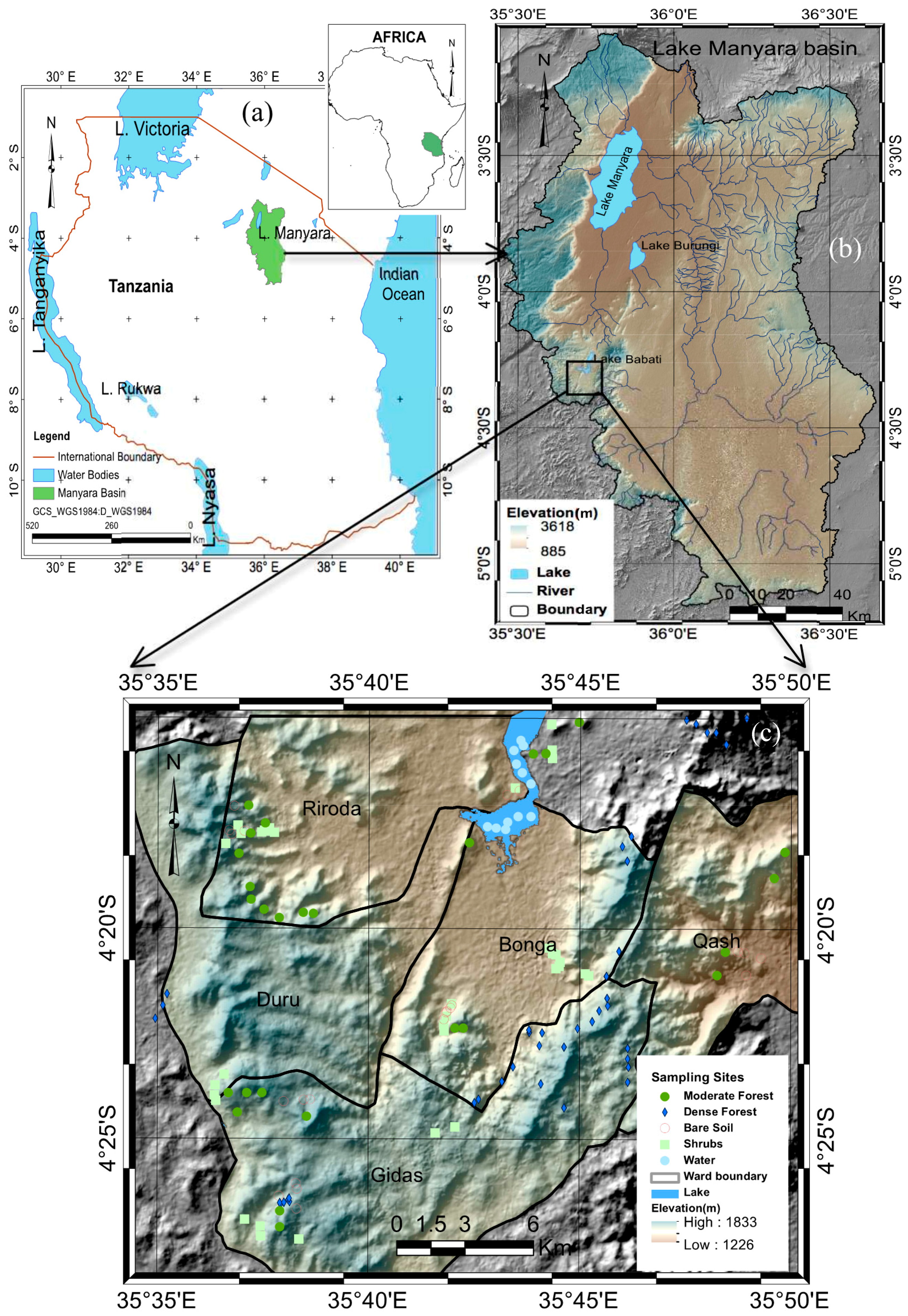
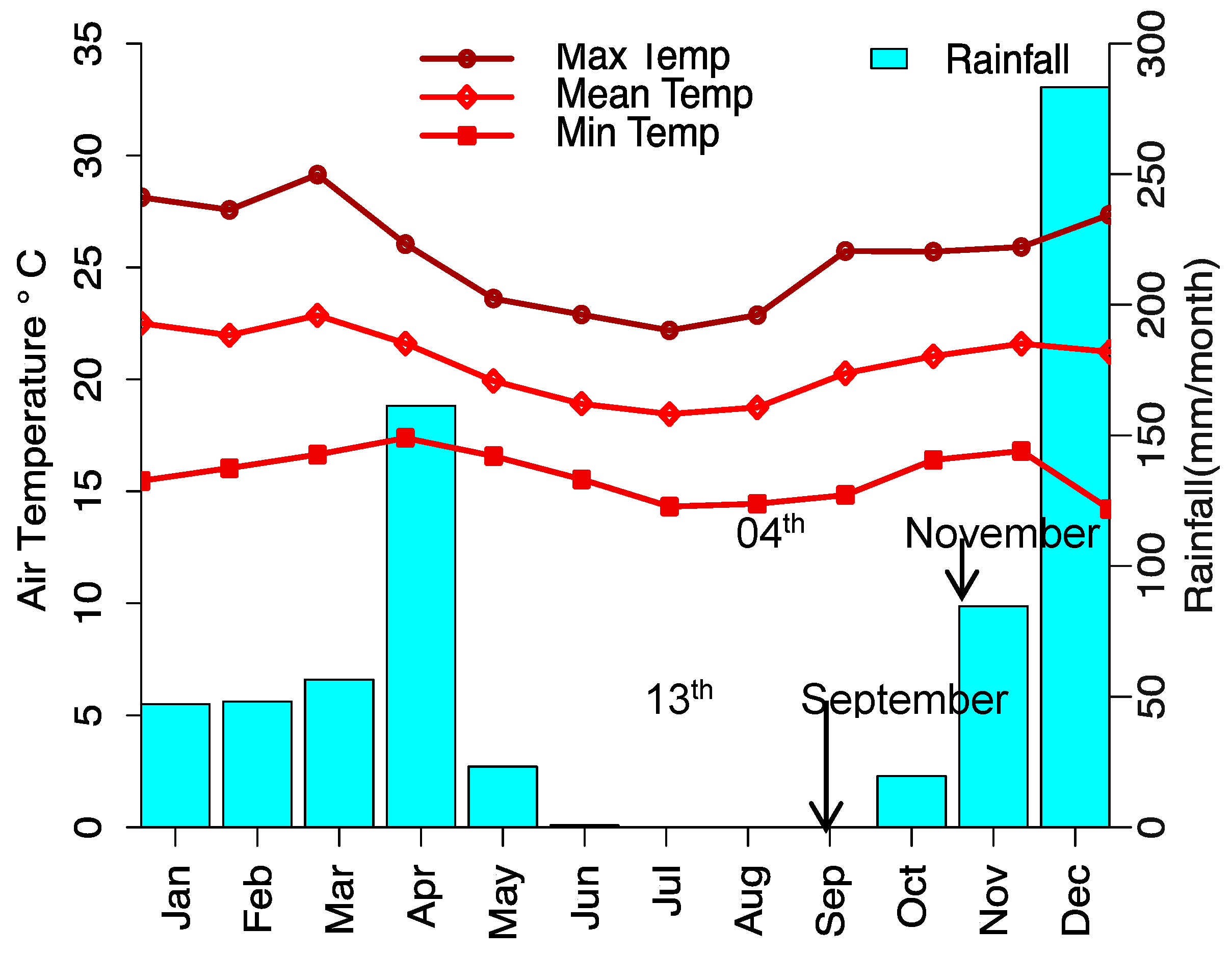
The study is based on Bereko and Duru-Haitemba forest reserves in Babati district, Manyara region, northern Tanzania. The reserves are located between latitude 4°15′ S and 4°30′ S, and between longitude 35°35′ E and 35°50′ E within lake Manyara basin (Figure 1). The mean annual rainfall is 700 mm/year and the average rainfall of about 60 mm/month (Figure 2). The mean monthly air temperature is 23 °C per day. The forest reserves can be categorized into six main land cover/use types: water (e.g., lakes and streams), shrubs, natural dense forest and moderate forests/woodlands (Table 1). The land categorized land cover types have been adopted from a 1996 land use/cover map of Singida (Sheet Index SB 36-4).
3. Datasets and Methods
3.1. Datasets
3.1.1. Remote Sensing Data
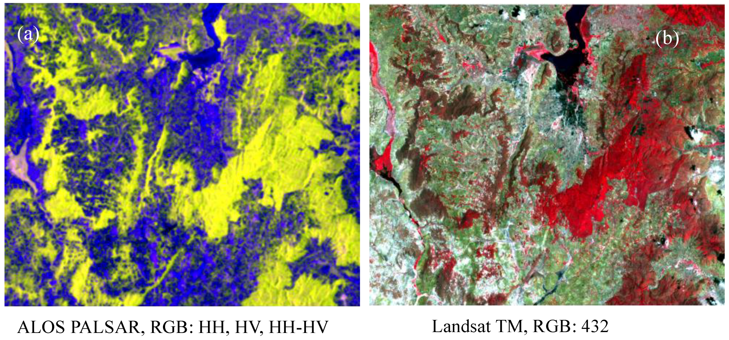
Both optical and SAR images (Table 2, Figure 3): Landsat 5 Thematic Mapper (TM) with a spatial resolution of 30 m and ALOS PALSAR L band [9] are applied, all images were acquired in 2009 dry season. Optical images acquired during the dry season are reported to be better and suitable for classification purposes in tropical environments [8,14]. The images acquired on the driest period of the year enhances spectral separability among classes. Six bands of the Landsat 5 TM image were used, these include visible and short wave infrared bands. Panchromatic and thermal infrared bands were not embraced in this research.
The ALOS/PALSAR scenes utilized were acquired in fine beam double mode (FBD). The HH and HV polarization scenes were extracted and obtained in slant range single look complex (SLC) format (level 1.1). Another dataset which has been utilized is the Shuttle Radar Topographic Mission (SRTM) Digital Elevation Model (DEM) 90m resolution [15,16] from US Geological Survey (USGS). The DEM was then resampled to 30 m spatial resolution using the nearest neighbor interpolation technique.
3.1.2. Ground Truth Data
Ground truth information was based on field data and on the inspection of spectral profiles (Figure 4). A set of Global Positioning System (GPS position) of points and knowledge-based information were captured for purposes of ground truthing in October 2009. The period is compatible with Duru Haitemba and Bereko forest reserve dry season (June to October/November) (Figure 2). Additionally, Apart from the GPS based sampling sites collection, a higher resolution image (i.e., Google Earth Image) and Normalized Difference Vegetation Index (NDVI) [17] were utilized for ground truthing purposes. A total of 143 sampling sites were selected and used during the selection of training and validation samples. This include water 12, bare land 22, moderate forest 35, dense forest 40, and shrubs 34 (Figure 1c). Among 143 sites, 96 sampling sites were selected based on Google Earth imagery especially within the lake and areas that were not accessible during the fieldwork and 47 sites were selected using a GPS device during the fieldwork. For every land cover class identified, five or more ground truthing sites were recorded on the area of interest using GPS. The points were then overlaid on the Landsat TM image for sampling of training and validation samples. Based on visual inspection of the higher resolution image and location of the collected samples in the field, training and validation samples were collected.
3.2. Methods
3.2.1. Image Pre-Processing
ALOS PALSAR dual polarization data scenes employed in this study were acquired at the slant range single look complex format. Both HH and HV polarizations of ALOS/PALSAR data from the single look slant range complex images were utilized. To improve radiometric resolution and to square the pixels in ground range geometry that is similar to the spatial resolution of Landsat data (e.g., 30 m); a multi-looking procedure of 9 × 2 (i.e., nine looks in azimuth and two looks in range) was applied to the scenes so as to transform them from slant range to ground range resolution [1,18,19]. The results were images with a 29.9 × 27.7 m2 resolution in range and azimuth respectively.
The refined Lee spatial filter [20] was adapted for speckle noise reduction. A 7 × 7 window size was selected based on minimum values of Speckle Suppression Index (SSI) [21,22] and Mean Preservation Speckle Suppression Index (MPSSI) [22].
To correct the data geometrically to allow integration of various datasets an orthorectification procedure using Shuttle Radar Topographic Mission (SRTM) Digital Elevation Model (DEM) 90 m resolution [15,16] was applied. All scenes were geo-referenced and registered in Universal Transverse Mercator (UTM) zone 36 projection system in the southern hemisphere. This is due to the fact that image fusion can only be executed for co-registered ALOS PALSAR and Landsat 5 TM scenes. All images were sampled to same pixel size, corresponding to the same location on the different images to be combined. After the geocoding process the intensity images were then transformed to their corresponding radar backscattering coefficients (sigma nought, in decibel (dB)). The digital number (DN) values were converted to normalized radar backscattering coefficients using Equation (1) [23]:
where is the radar backscattering coefficient, CF is a calibration factor (CF = −83 dB), I and Q are the real and imaginary parts of the complex SAR image DN value.
Radiometric terrain correction was also applied to all ALOS PALSAR scenes so as to account for topographic effects on the radar backscattering coefficients. The improved backscattering in gamma-nought was attained from the sigma-nought value based on Equation (2) [2,24,25].
where by is topographic normalized radar backscattering coefficient, is the radar backscattering coefficient, is PALSAR pixel size for a theoretical flat terrain, is true local PALSAR pixel size for the mountainous terrain, is local incidence angle and is radar incidence angle at the image center. The exponent n is the optical canopy depth and ranges between 0 and 1. It is a site-specific factor and difficult to obtain in practice, therefore it is set to 1 [2].
Polarimetric features like alpha angle (α), entropy (H) and anisotropy (A) were also computed based on Alpha-Entropy decomposition proposed by Cloude and Pottier [26]. The features were computed as derivatives of SAR backscattering ready for the integration of surface reflectance, backscattering and their derivatives. Cloude and Pottier have proposed a method of the extraction of mean diffusion based on eigenvalues/eigenvectors decomposition of the coherence matrix in order to characterize scattering interactions of the beams with the targets. High values of alpha stand for volume or multiple scattering mechanisms and low values associate with surface scattering. Entropy indicates the randomness or statistical disorder of the target [26].
After orthorectification of the Landsat-5 TM data, the digital numbers were then converted to sensor radiance considering both gain and bias of the sensor. The sensor radiance was then converted to surface reflectance using Atmospheric and Topographic Correction 3 (ATCOR3) [27]. The data were also topographically normalized using ATCOR3 [2]. In ATCOR3 the topographic normalization algorithm is developed by [28] and the atmospheric correction functions are based on MODTRAN4. MODTRAN4 is an atmospheric correction package accounts for path scattered radiance, absorption, and adjacency effects [29,30].
3.2.2. Indices and Textural Parameters Computation
Several indices that include vegetation indices (VI), PCA and texture variables were derived using Landsat-5 TM and SAR data to evaluate their influence on land cover classification. VI, PCA and texture measures of both optical and SAR data are extensively applied for land cover classification [2].
Three key SAR indices were extracted using the amplitude backscatter values of HH and HV polarizations from the ALOS PALSAR data. This includes SAR quotient bands HH/HV and HV/HH [31] and Radar Forest Deforestation Index (RFDI) [32] and the Grey-Level Co-Occurrence Matrix (GLCM) [33] textural feature measures (Table 3). RFDI is a ratio between the power of the HH and HV polarizations meant to measure the strength of the double bounce term and distinguish various vegetation types (i.e., HH − HV/HH + HV) [32].
The GLCM textures were retrieved for ALOS PALSAR and Landsat scenes, respectively. The GLCM texture measures have been widely applied in previous researches on land cover categorization [2]. The GLCM texture measures make use of grey-tone spatial dependence matrix to quantify texture features, which are utilized for classification purpose. The GLCM expresses texture in a user defined moving window and considers for this moving window the spatial co-occurrence of pixel grey levels [34]. The size of the kernel selected affects the role of GLCM textures in land cover classification [2,3]. Therefore, choosing a suitable kernel size for texture quantification is essential. This is due to the fact that smaller kernel size may exaggerate variations while larger kernel size cannot efficiently quantify texture because of smoothing [3,34,35]. For each band eight textural variables were computed namely mean (mea) entropy (ent), correlation (cor), variance (var), homogeneity (hom), dissimilarity (dis), contrast (con) and second moment (sec) (Table 3). A moderate kernel size of 9 × 9 was selected based on the separabilities of different land cover classes.
Additionally, for Landsat 5 TM image; the Normalized Vegetation Index (NDVI), Soil adjusted Vegetation Index (SAVI) [36], Soil leaf Area Vegetation Index (SLAVI) [37] and principal component analysis (PCA) [38] were retrieved (Table 3). NDVI provide greenness information to indicate vegetated and non-vegetated areas in the classification system. The PCA is a data compression method that reduces dimensionality of the multidimensional data sets. In PCA the axes of the origin feature space are rotated in such a way that the data set are presented unrelated in a new component space. The first PC band consists of the largest fraction of the dataset variance while the last PC band consists of the smallest fraction of the dataset variance [4,38]. PC band lacks redundancy of data given the orthogonal components and reduces complexity in image classification [39].
Generally, in this study SAR and Landsat data derivatives like GLCM textural bands, PCA, NDVI/RFDI and quotient bands are integrated in the classification system and they show a significant impact. This is due to the fact that, they contribute key information to aid image-processing tasks such as segmentation, feature extraction and object recognition.
3.2.3. Image Synthesis
Following image pre-processing various procedures were performed so as to prepare the multi-sensor input bands for the subsequent land cover categorization and forest mapping. Image synthesis is a process, which is used to combine information from multiple images of the same scene so as to acquire more information from the integration. It is a combination of different digital images to obtain a new image and obtain more information that can be separately derived from any of the origin image [4,11,12]. The resulting new image is more suitable for human and machine perception or further image-processing tasks such as segmentation, feature extraction and object recognition [41].
Image synthesis can be achieved using two different methods: image fusion or multi-sensor integration. The first method combines the data contained in two or more image bands to form a new synthetic image or group of images. The second method combines n images in n different layers algorithmically, without creating a new set of images [4,11,12]. In this study, the second image integration approach has been adapted. Image integration may improve reliability by using redundant information and improves capability by using complementary information [11].
3.2.4. Sampling and Land Cover Type Determination
Identification of the representative homogeneous areas for land cover classes (Table 1) on the study area was carried out based on sampling sites (Figure 1c). The sampling sites (both training and validation) were selected based on ground truth data for land cover type information, GPS based point locations and knowledge based information acquired on the site. Unsupervised classification and visual interpretation of the images and Google Earth images were performed to ensure collect selection of the training and validation samples. Additionally, NDVI values [17], were utilized also in order to obtain optimal classification results [42]. Additionally, unsupervised classification and visual interpretation of these scenes were performed to ensure the correctness of the identified land cover type.
About 590 pixels within the study area were selected to serve as training and testing samples during the classification process. The samples were then divided into two groups; one for classification (training/70% of the dataset, 413 pixels) and the second was for accuracy assessment (validation/30% of the dataset, 177 pixels).
Spectral separability analysis was done using the Jeffries-Matusita distance [38]. The Jeffries-Matusita distance is widely used in the field of remote sensing to determine the statistical distance between two training samples. The separability values ranges from 0 to 2.0 and indicate how well the selected training site pairs are statistically separate. Values greater than 1.9 indicate that the training pairs have good separability [38]. Low training site signature separability is generally caused by inappropriate combinations of image bands and/or training site; these have large internal variability within each class.
3.2.5. Classification Algorithm and Approach
For land cover categorization of the independent bands and combined ALOS PALSAR/Landsat data and their derivatives a Support Vector Machine (SVM) classifier [1,2,43,44] was utilized.
The SVM is basically a binary class classification method based on machine learning and using support vector in the data classification. SVM was chosen due to the fact that, it is a non-parametric statistical learning approach which is known for resolving complex (e.g., multimodal) class distribution in high dimensional feature spaces. It makes use of non-linear kernel functions and it deals with noise and class confusion via the regularization technique [1,43]. Linear, polynomial, radial basis function and sigmoid are the four common kernels available in remote sensing packages. A careful selection of parameter setting can improve the performance of the SVM [45]. The Gaussian radial basis kernel function and a penalty parameter of 100 were selected based on trial and error. However, the kernel and penalty parameter selected are recommended to be the best for land cover classification [45].
To run the classification process and assess the potential of integration of backscattering, surface reflectance and their derivatives. The datasets were categorized into three major groups A–C (Table 4), Category A, consists of surface reflectance bands from Landsat 5 TM image and its derivatives (i.e., Vegetation index, GLCM textures and PCA). Category B, comprises of individual ALOS PALSAR backscattering and derivatives. Category C, involve the fusion of surface reflectance, backscattering and their derivatives.
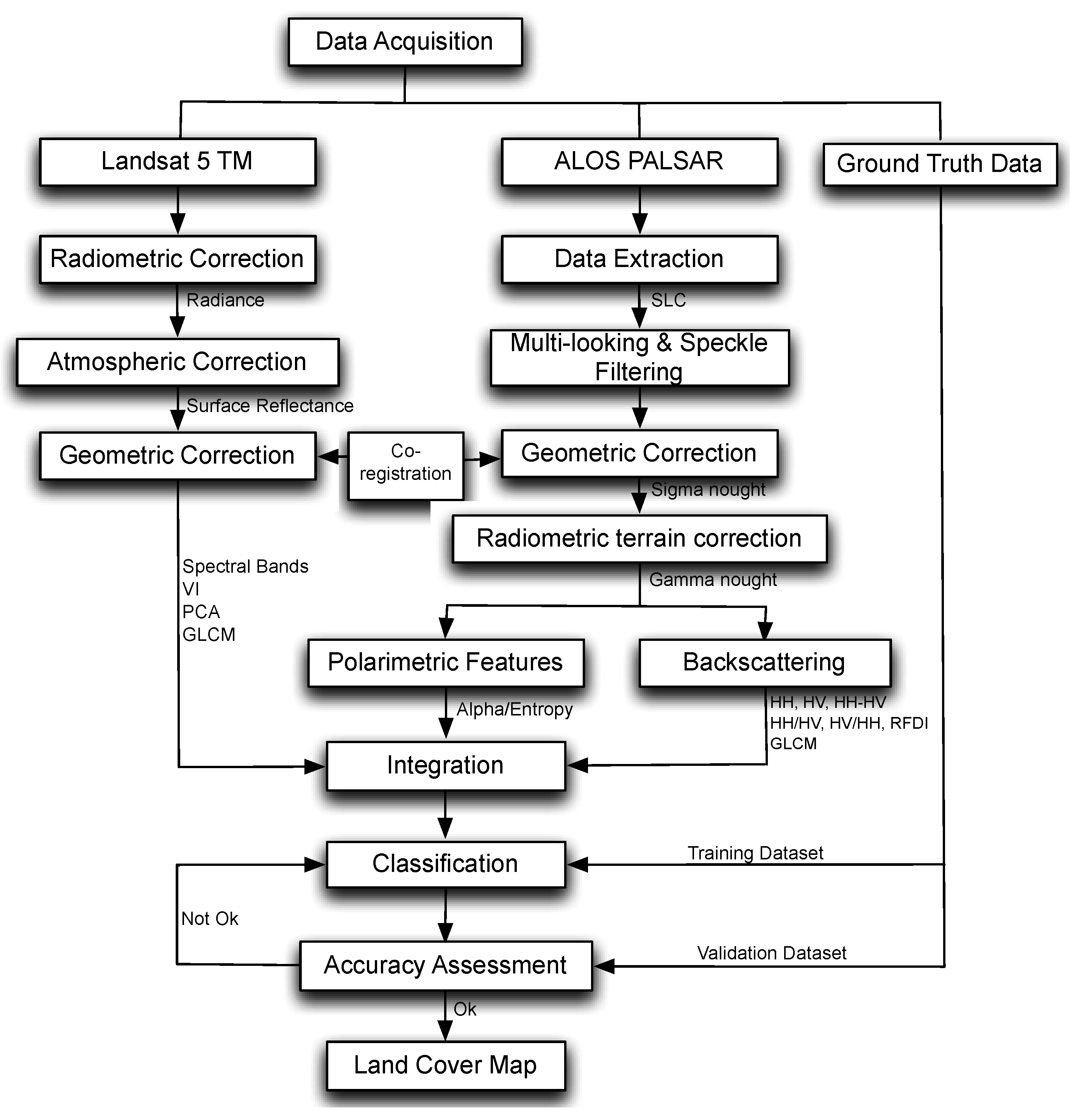
However, to maximize the classification accuracy the best blend of textures, indices and features were identified. This is due to the fact that, not all the derived features are useful for land cover classification and some of them may have similar information [2,3]. Initially textural bands, indices and polarimetric features with high separability were chosen. Then the correlation among various textural bands, indices and polarimetric features was checked to decrease data redundancy [2,3]. Finally, the selection of relevant textural bands, indices and polarimetric features was carried out based on trial and error classification. Figure 4 illustrates the overall simplified flowchart of the proposed methodology.
3.2.6. Classification Accuracy Assessment
To test the capability of non-parametric classifiers compared to the maximum likelihood classification approach a validation dataset was used for accuracy assessment. The accuracy assessment was performed in terms of individual error matrices for the classified surface reflectance bands, backscattering and their derivatives for all groups of data generated for the classification scenarios (Table 4). Four terms that describe the classification accuracy were computed (i.e., User’s Accuracy (UA), Producer’s Accuracy (PA), Overall Accuracy (OA) and Kappa Coefficient (κ)) [46]. Producer’s accuracy is used to estimate the omission error to a certain class and it is the probability that a reference site has been classified correctly. User’s accuracy is used to estimate the commission error and it is the probability that a pixel classified on the image signifies the actual class on the ground. The overall accuracy is the percentage of the pixels that have been classified correctly in the validation dataset [46].
Furthermore, for each land cover class, F1 score index [47], that merges producer’s and user’s accuracy into a fused quantity, was computed (Equation (3)). This quantity enables a better evaluation of the land cover class-wise accuracies. The score varies between 0 and 1 where by 0 signifies the worst results, and 1 is the best accuracy achieved.
To evaluate the influence of surface reflectance and backscattering derivatives on the classification accuracy the two-sample t-test [48] was applied on the F1 score indexes attained. The two-sample t-test assesses whether two samples means are similar. A difference in mean indicates that the two samples are dissimilar. The test is normally applied when the test makes use of a small sample size, the variances of two normal distributions are unknown and the experimentation involve a small sample size.
4. Results
4.1. Backscattering, Surface Reflectance and Their Derivatives Description
SAR backscattering showed the highest values on dense forest and moderate forest compared to shrubs, bare soil and water (Figure 5a). Relating the backscattering values in co-polarized band (HH) and cross-polarized band (HV) displays that dense forest, moderate forest and classes have higher backscattering in HV polarized band (Figure 5a, Table 5). In general, backscattering values are higher in the dense forest and moderate forest covers due to the predominance of surface scattering as indicated in Figure 6. Water and bare soil covers present lower backscattering values (Figure 5a, Table 5).
The Alpha-Entropy decomposition of ALOS PALSAR was generated from eigenvalues-based target decomposition. In the alpha-entropy plane, lower values of alpha are depicted with relatively higher entropy values especially for dense forest, moderate forest and shrub land cover classes (Figure 6, Table 5). Forest land cover classes (both dense and moderate forest) demonstrate higher alpha values compared to other classes under study (Figure 6b). Landsat surface reflectance values of the training samples indicates higher values on the near infrared (NIR) band for the dense forest cover with lower values in Red band (Figure 5b). Water indicates higher values for Green band and lower values in other wavelength bands (Figure 5b).
4.2. Spectral Separability Assessments
A separability analysis was conducted to assess whether the identified categories of the data could clearly differentiate various land cover types under study. Category A and C have high separability values (Table 6). This indicates a good separation between land cover classes. In category B, especially subgroup B1, the separability values between land cover classes are very low. This demonstrates that various land cover classes are hard to differentiate with dual polarimetric SAR data. Including backscattering derivatives like RFDI, GLCM textures, quotient bands and other derived features improve the land cover separability for instance from 0.34 in subgroup B1 to 1.57 in subgroup B2 for the SH-BS land cover pair (Table 6). In all data categories separability values for DF-SH, DF-WA and DF-BS land cover pair are higher (Table 6).
4.3. Evaluation of Classification Results for Different Data Categories
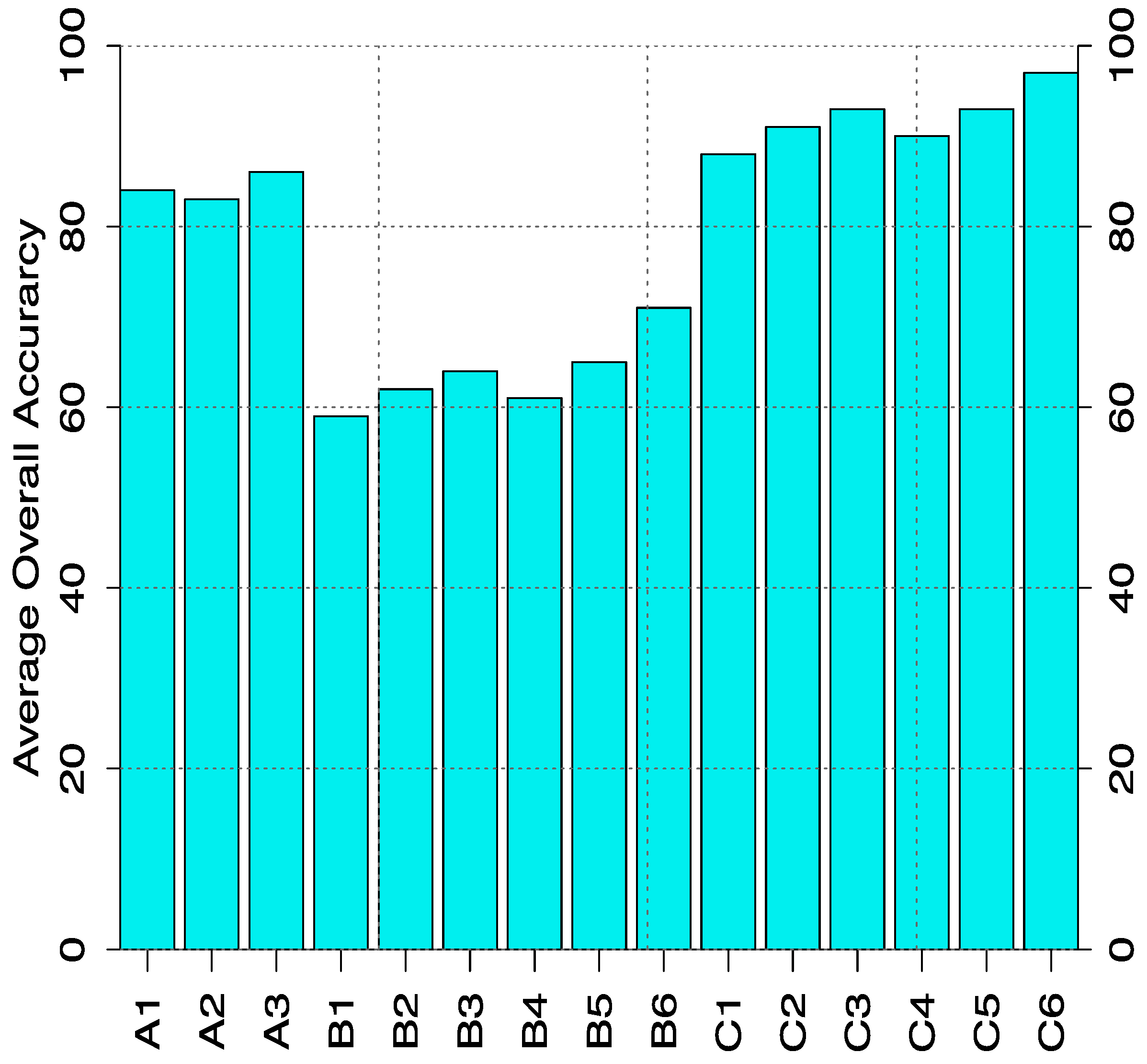
The classification results attained based on different data categories (A–C), for Landsat, ALOS PALSAR, their derivatives and integration are presented in Table 7 and Figure 7 respectively. Table 7 depicts classification results of the SVM classifiers for each data categories (A–C) in terms of the PA, UA and F1 score index. The results are for all land cover classes under study. In Table 7 both category A and C provides the best classification accuracy in terms of PA, UA and F1 score index for all land cover types. Category B indicates poor PA for dense forest and bare soil covers, with lower UA values for dense forest, moderate forest and bare soil land cover classes. Lower F1 score index values are obtained for dense forest and bare soil covers. The overall classification accuracy for all data categories are indicated in Figure 7.
4.4. Landsat TM and ALOS PALSAR Classification Accuracy
Table 7 and Figure 7 provide a summary of the classification results attained for all data categories. In category A, PA; UA and F1 score values for all land cover classes are higher (PA and UA values ≥ 92%). Categorization of Landsat surface reflectance and its derivatives, subgroup A3 provides the highest overall accuracy value for the data category A (OA = 86%) (Figure 7). This shows the influence of surface reflectance based derivatives on the classification accuracy. Landsat TM based classification results shows that medium resolution satellite data has the potential to categorize land cover efficiently (Figure 7). The results were improved substantially on combination of surface reflectance with the derivatives like PCA, VI and GLCM textures.
In-group B, subgroup B1 SAR backscattering values for HH and HV polarization bands are classified independently attaining an overall accuracy (OA = 59%) (Figure 7). For subgroup B2, RFDI, quotient bands (HH/HV, HV/HH), HH-HV, polarimetric features (alpha and entropy) as well as GLCM textures are included. The overall classification accuracy attained for B2 (OA = 62%). For subgroup B3, HH, RFDI, HH/HV, HV/HH, HH-HV bands are included yielding an overall accuracy (OA = 64%). For data category B4, HH and selected GLCM texture bands of HH and HV (cor_HH, cor_HV, mea_HH, var_HH, sec_HH, sec_HV) are included and an overall classification accuracy (OA = 56%) is achieved. In category B5, HH and polarimetric features (Alpha and entropy) are included for the classification resulting in to overall accuracy (OA = 65%). For subgroup B6, HH, HH/HV, HV/HH, alpha, entropy, and GLCM textures bands (cor_HH, cor_HV, mea_HH, var_HH, sec_HH, sec_HV) are includes for the classification producing an overall accuracy (OA = 71%). The category with SAR backscattering only, B1 depicts the lowest overall classification accuracy (OA = 59%) while B6 presents the highest overall classification accuracy in this category (OA = 71%. Assessments among individual data category classification indicates higher accuracies in subgroup B6 compared to B1, indicating the influence of the inclusion of SAR derivatives (Figure 7). Examining on the PA, UA and F1 score values, it can be observed that in data category B, all subgroups (B1–B6) cannot differentiate the forest covers (DF and MF) and bare soil classes properly.
4.5. Integration of TM and ALOS PALSAR
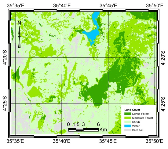
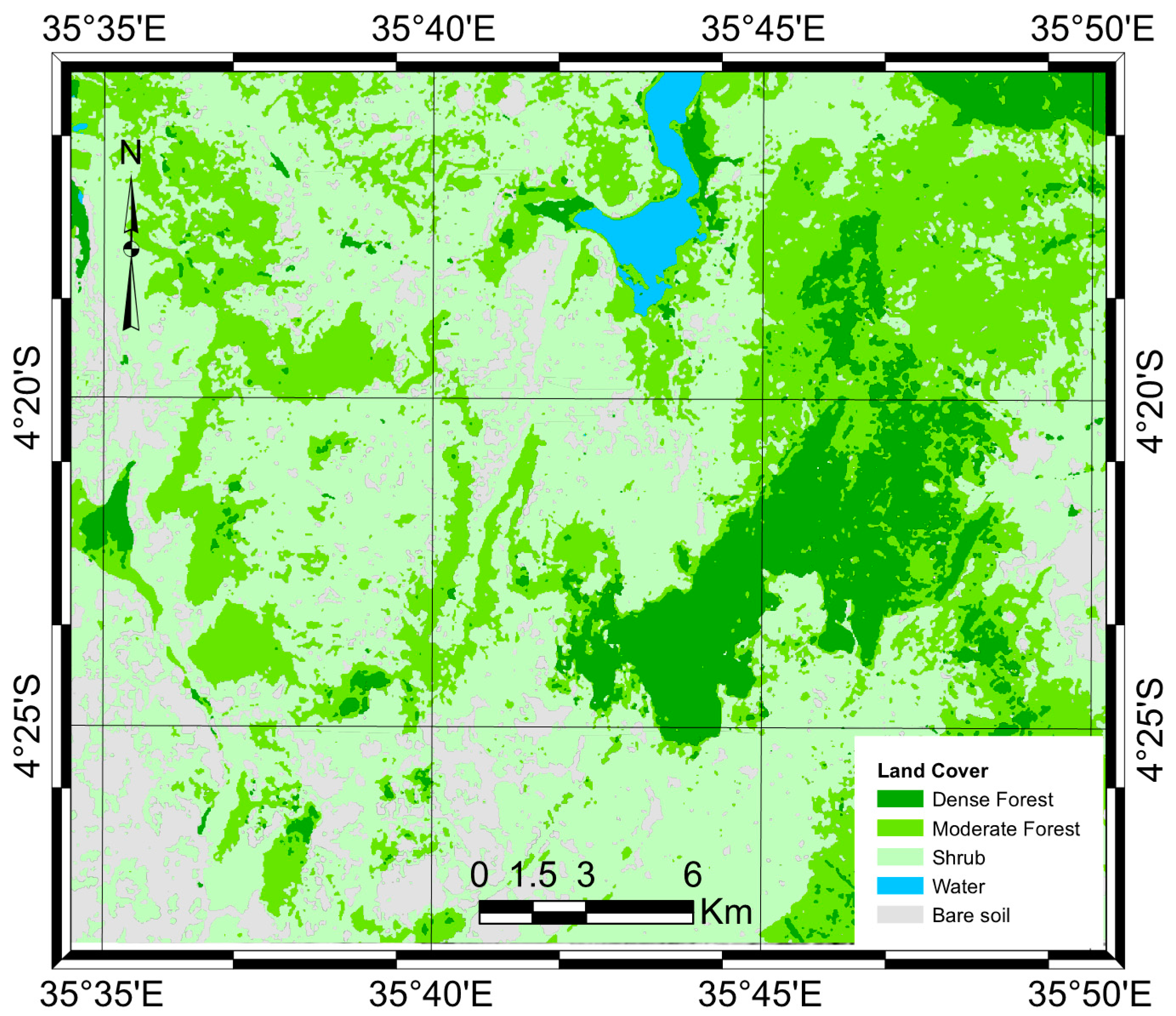
In the joint processing, ALOS PALSAR and Landsat TM data are classified together. Data category C is utilized in this case. The results obtained in this category indicated that the average overall classification accuracies of the data in subgroup C1–C6 ranges between 85% and 95%. Combination of surface reflectance, backscattering and their derivatives improves the results significantly, e.g., subgroup C1–C6) (Figure 7). However, integration of Landsat TM and ALOS PALSAR improve the overall classification accuracy slightly. The classification accuracy of the data category with a combination of surface reflectance and backscattering (C1) produces an average overall accuracy of 91%. The classification accuracy attained in this subgroup C1 is more or less same as the one obtained using surface reflectance and its derivative, subgroup A3 (Figure 7). SAR derivatives combining with Landsat surface reflectance derivatives, improve the results substantially as indicates in subgroup C2–C6 (Figure 7). The highest overall classification accuracy was attained based on a joint processing of SAR backscattering, TM surface reflectance and selected bands of their derivatives (average OA = 95%). Generally, this indicates that integration of surface reflectance, backscattering and their derivatives improves the overall classification accuracy. Figure 8 present a classified land cover map, displaying the forest cover distribution over the study area. The map was produced using subgroup C6 of the dataset.
5. Discussion
In this research, a separate and joint processing of Landsat TM and ALOS PALSAR has been executed. Separability values of various land cover classes using Landsat TM data, and the combination of TM and SAR data are higher compared to mere SAR data. Higher separability values using a blend of Landsat ETM+ and SAR were also obtained by Attarchi and Gloaguen [2]. For SAR data we observe lowest separability values especially between dense forest and moderate forest cover classes (Table 6).
Independent and joint processing of Landsat TM surface reflectance and its derivatives show satisfactory results on land cover and forest mapping (Figure 7 and Table 7). When classifying surface reflectance independently, data category A1 low value of the overall classification accuracy was attained compared to the integration of surface reflectance and derivatives, category A3 (Figure 7). The results on Land cover classification using SAR backscattering (HH and HV), category B1 are not adequate (OA = 59%). Adding SAR derivatives like quotient bands RFDI, GLCM textures and polarimetric features (Alpha and Entropy) to backscattering increase the classification accuracy significantly data category B3 (OA = 71%). SAR backscattering derivatives independently provides an overall classification accuracy of 62%. Combining backscattering, RFDI and quotient bands (HH/HV, HV/HH) increases the overall accuracy classification to 64%. The joint processing of backscattering and GLCM textures increases the overall classification accuracy to 61%, 2% higher than when classifying backscattering alone. SAR backscattering and polarimetric features increase the overall classification value to 65% (Figure 7). However, despite the attained satisfactory classification accuracy results based on SAR dataset; it does not surpass the accuracy achieved using Landsat data. This indicates that in the absence of optical data, SAR data can be utilized as an alternative for land cover classification purposes, especially in tropic environment where cloud cover is a huge problem. This suggests that SAR data could be utilized perfectly for environmental monitoring in the tropics. Some of the previous studies attained similar results regarding SAR data compared to optical dataset [1,2].
The joint processing of Landsat TM and ALOS PALSAR increases the overall classification accuracy meaningfully, category C6 (OA = 97%). Comparing to category A3, Landsat surface reflectance and its derivatives independently (OA = 86%), the increase of 11% is attained on joint processing of Landsat surface reflectance, SAR backscattering and their derivatives, However, the enhancement is not that substantial and the result attained in some of the data categories is very close to the original Landsat classification (Figure 7). For instance the combination of surface reflectance and backscattering, category C1 improves the classification accuracy to 88%, 4% higher compared to the classification of Landsat surface reflectance independently, data category A1. The joint processing of SAR backscattering and Landsat TM derivatives, category C2, increases the classification accuracy to 91% while the joint processing of polarimetric features and Landsat based derivatives, category C3, improves the overall classification accuracy to 93%. SAR GLCM texture measures and Landsat based derivatives increases the classification accuracy to 91%. The joint processing of SAR backscattering and Landsat TM surface reflectance based derivatives, data category C5, improves the overall classification accuracy to 95%. Attarchi and Gloaguen [2], also obtained similar results when classifying mountainous forest.
6. Conclusions
The potential of the integration of Landsat TM and ALOS PALSAR data has been experimented with. Based on the results attained it could be concluded that independent processing of Landsat TM surface reflectance produces satisfactory results for forest cover and land cover mapping. SAR backscattering independently results in to unsatisfactory classification results.
Landsat TM surface reflectance and its derivatives increase the classification accuracy significantly (Subgroup A3). The inclusion of SAR backscattering and derivatives especially (subgroup B3–B5) increases the overall classification accuracy at the 5% significance level when compared with backscattering alone (subgroup B1). The integration SAR backscattering and its derivatives (category B) did not surpass the classification accuracy attained when using both surface reflectance alone and the combination of surface reflectance and derivatives (category A). However, SAR backscattering and derivatives could be an alternative source of data for land cover categorization in tropical regions where cloud cover is a huge problem.
On the integration of SAR backscattering, Landsat surface reflectance and their derivatives increase classification accuracy slightly. The improvements are observed when using data category C where the average overall accuracy for all classifiers reached up to 97%. Therefore it can be concluded that integration of ALOS PALSAR and optical data improve the classification accuracies of land cover and forest mapping substantially; and the joint processing of the data indicates their great potential in environmental monitoring. In future further research using data acquired by new sensors like ALOS PALSAR-2, Landsat-8 and Sentinel-2 should be carried out to evaluate their potential in land cover categorization and mapping for environmental monitoring.
Acknowledgments
The author thanks Veraldo Liesenberg for facilitating the acquisition of ALOS PALSAR L band data. The data was acquired under Cat.1-Proposal 6242 through the European Space Agency (ESA) Third Party Mission. The Landsat TM data was downloaded from the US Geological Survey (USGS) website.
Conflicts of Interest
The author declares no conflict of interest.
Abbreviations
The following abbreviations are used in this manuscript:
| ALOS | Advanced Land Observing Satellite |
| ATCOR3 | Atmospheric and Topographic Correction 3 |
| BS | Bare soil |
| con | Contrast |
| Cor | Correlation |
| DEM | Digital Elevation Model |
| DF | Dense Forest |
| dis | Dissimilarity |
| ent | Entropy |
| ETM | Enhanced Thematic Mapper |
| GLCM | Grey Level Co-Occurrence Matrix |
| GPS | Global Positioning System |
| KC | Kappa Coefficient |
| MF | Moderate Forest |
| mea | Mean |
| MIRI | Middle Infrared Index |
| MPSSI | Mean Preservation Speckle Suppression Index |
| NDVI | Normalized Difference Vegetation Index |
| OA | Overall Accuracy |
| PA | Producer’s Accuracy |
| PALSAR | Phased Array type L-band Synthetic Aperture Radar |
| PCA | Principal Component Analysis |
| PolSAR | Polarimetric Synthetic Aperture Radar |
| RFDI | Radar Forest Deforestation Index |
| RS | Remote Sensing |
| SAR | Synthetic Aperture Radar |
| SAVI | Soil adjusted Vegetation Index |
| sec | Second Moment |
| SH | Shrub |
| SLAVI | Soil leaf Area Vegetation Index |
| SRTM | Shuttle Radar Topographic Mission |
| SSI | Speckle Suppression Index |
| SVM | Support Vector Machine |
| TM | Thematic Mapper |
| UA | User’s Accuracy |
| UTM | Universal Transverse Mercator |
| var | Variance |
| VI | Vegetation Index |
| WA | Water |
References
- Liesenberg, V.; Gloaguen, R. Evaluating SAR polarization modes at L-band for forest classification purposes in Eastern Amazon. Int. J. Appl. Earth Obs. Geoinf. 2013, 21, 122–135. [Google Scholar] [CrossRef]
- Attarchi, S.; Gloaguen, R. Classifying complex mountainous forests with L-Band SAR and Landsat data integration: A comparison among different machine learning methods in the hyrcanian forest. Remote Sens. 2014, 6, 3624–3647. [Google Scholar] [CrossRef]
- Li, G.; Lu, D.; Moran, E.; Dutra, L.; Batistella, M. A comparative analysis of ALOS PALSAR L-band and RADARSAT-2 C-band data for land-cover classification in a tropical moist region. ISPRS J. Photogramm. Remote Sens. 2012, 70, 26–38. [Google Scholar] [CrossRef]
- Amarsaikhana, D.; Blotevogelb, H.H.; van Genderenc, J.L.; Ganzoriga, M.; Gantuyaa, R.; Nerguia, B. Fusing high-resolution SAR and optical imagery for improved urban land cover study and classification. Int. J. Image Data Fusion 2010, 1, 83–97. [Google Scholar] [CrossRef]
- Vaglio Laurin, G.; Liesenberg, V.; Chen, Q.; Guerriero, L.; del Frate, F.; Bartolini, A.; Coomes, D.; Wilebore, B.; Lindsell, J.; Valentini, R. Optical and SAR sensor synergies for forest and land cover mapping in a tropical site in West Africa. Int. J. Appl. Earth Obs. Geoinf. 2013, 21, 7–16. [Google Scholar] [CrossRef]
- Wijaya, A.; ReddyMarpu, P.; Gloaguen, R. Discrimination of peatlands in tropical swamp forests using dual-polarimetric SAR and Landsat ETM data. Int. J. Image Data Fusion 2010, 1, 257–270. [Google Scholar] [CrossRef]
- Strömquist, L.; Backéu, I. Integrated landscape analyses of change of miombo woodland in Tanzania and its implication for environment and human livelihood. Geografiska Annaler: Series A. Phys. Geogr. 2009, 91, 31–45. [Google Scholar]
- Liesenberg, V.; Galvão, L.S.; Ponzoni, F.J. Variations in reflectance with seasonality and viewing geometry: Implications for classification of Brazilian savannah physiognomies with MISR/Terra data. Remote Sens. Environ. 2007, 107, 276–286. [Google Scholar] [CrossRef]
- Rosenqvist, A.; Shimada, M.; Ito, N.; Watanabe, M. ALOS/PALSAR: A pathfinder mission for global-scale monitoring of the environment. IEEE Trans. Geosci. Remote Sens. 2007, 45, 3307–3316. [Google Scholar] [CrossRef]
- Lu, D.; Li, G.; Moran, E.; Dutra, L.; Batistella, M. A comparison of multisensor integration methods for land Cover classification in the Brazilian Amazon. GISci. Remote Sens. 2011, 48, 345–370. [Google Scholar] [CrossRef]
- Pohl, C.; Van Genderen, J.L. Multisensor image fusion in remote sensing: Concepts, methods and applications. Int. J. Remote Sens. 1998, 19, 823–854. [Google Scholar] [CrossRef]
- Furtado, L.S.A.; Silva, T.S.F.; Fernandes, P.J.F.; Novo, E.M.L.M. Land cover classification of Lago Grande de Curuai floodplain (Amazon, Brazil) using multi-sensor and image fusion techniques. Octa Amazon. 2015, 45, 195–202. [Google Scholar] [CrossRef]
- Ghulam, A.; Porton, I.; Freeman, K. Detecting subcanopy invasive plant species in tropical rainforest by integrating optical and microwave (InSAR/PolInSAR) remote sensing data, and a decision tree algorithm. ISPRS J. Photogramm. Remote Sens. 2014, 88, 174–192. [Google Scholar] [CrossRef]
- Ratana, P.; Huete, A.R.; Ferreira, L. Analysis of Cerrado physiognomies and conversion in the MODIS seasonal–temporal domain. Earth Interact. 2005, 9, 1–22. [Google Scholar] [CrossRef]
- Rabus, B.; Eineder, M.; Roth, A.; Baler, R. The shuttle radar topography mission—A new class of digital elevation models acquired by spaceborne radar. ISPRS J. Photogramm. Remote Sens. 2003, 57, 241–262. [Google Scholar] [CrossRef]
- Jarvis, A.; Reuter, H.I.; Neson, A.; Guevara, E. Hole-filled SRTM for the globe Version 4. In CGIAR-SXI SRTM 90m Database 2008. Available online: http://srtm.csi.cgiar.org (accessed on 15 July 2011).
- Rousel, J.W.; Haas, R.H.; Schell, J.A.; Deering, D.W. Monitoring vegetation systems in the great plains with ERTS. In Proceedings of the 3rd ERTS Symposium, Washington, DC, USA, 10–14 December 1973.
- Lee, J.S.; Hoppel, K.W.; Mango, S.A.; Miller, A.R. Intensity and phase statistics of multilook polarimetric and interferometric SAR imagery. IEEE Trans. Geosci. Remote Sens. 1994, 32, 1017–1028. [Google Scholar]
- Cantalloube, H.; Nahum, C. How to compute a multi-look sar image? In Proceedings of the Working Group on Calibration and Validation, Toulouse, France, 26–29 October 1999.
- Lee, J.S.; Wen, J.H.; Ainsworth, T.L.; Chen, K.S.; Chen, A.J. Improved sigma filter for speckle filtering of SAR imagery. IEEE Trans. Geosci. Remote Sens. 2009, 47, 202–213. [Google Scholar]
- Shamsoddini, A.; Trinder, J.C. Image texture preservation in speckle noise suppression. In Proceedings of the ISPRS TC VII Symposium—100 Years ISPRS, Vienna, Austria, 5–7 July 2010.
- Dellepiane, S.G.; Angiati, E. Quality assessment of despeckled SAR images. In Proceedings of the 2011 IEEE International Geoscience and Remote Sensing Symposium (IGARSS), Vancouver, BC, Canada, 24–29 July 2011; pp. 3803–3806.
- Shimada, M.; Isoguchi, O.; Tadono, T.; Isono, K. PALSAR radiometric and geometric calibration. IEEE Trans. Geosci. Remote Sens. 2009, 47, 3915–3932. [Google Scholar] [CrossRef]
- Castel, T.; Beaudoin, A.; Stach, N.; Stussi, N.; leToan, T.; Durand, P. Sensitivityofspace-borne SAR data to forest parameters over sloping terrain. Theory and experiment. Int. J. Remote Sens. 2010, 11, 2351–2376. [Google Scholar]
- Ulander, L.M. Radiometric slope correction of synthetic-aperture radar images. IEEE Trans. Geosci. Remote Sens. 1996, 34, 1115–1122. [Google Scholar] [CrossRef]
- Cloude, S.R.; Pottier, E. An entropy based classification scheme for land applications of polarimetric. IEEE Trans. Geosci. Remote Sens. 1997, 35, 68–78. [Google Scholar] [CrossRef]
- Richter, R.; Schläpfer, D. Atmospheric/Topographic Correction for Satellite Imagery (ATCOR-2/3 User Guide, Version 8.2 BETA); German Aerospace Center, Remote Sensing Data Center: Wessling, Germany, 2012. [Google Scholar]
- Richter, R. Correction of atmospheric and topographic effects for high spatial resolution satellite imagery. Int. J. Remote Sens. 1997, 18, 1099–1111. [Google Scholar] [CrossRef]
- Adler-Golden, S.M.; Matthew, M.W.; Bernstein, L.S.; Levine, R.Y.; Berk, A.; Richtsmeier, S.C.; Acharya, P.K.; Anderson, G.P.; Felde, G.; et al. Atmospheric correction for shortwave spectral imagery based on MODTRAN4. Proc. SPIE 1999, 3753, 61–69. [Google Scholar]
- Felde, G.W.; Anderson, G.P.; Cooley, T.W.; Matthew, M.W.; Adler-Golden, S.M.; Berk, A.; Lee, J.S. In Analysis of hyperion data with the FLAASH atmospheric correction algorithm. In Proceedings of the 2003 IEEE International Geoscience and Remote Sensing Symposium, Toulouse, France, 21–25 July 2003; pp. 90–92.
- Wijaya, A.; Gloaguen, R. Fusion of ALOS Palsar and Landsat ETM data for land cover classification and biomass modeling using non-linear methods. In Proceedings of the 2009 IEEE International Geoscience and Remote Sensing Symposium, Cape Town, South Africa, 12–17 July 2009.
- Mitchard, E.T.A.; Saatchi, S.S.; White, L.J.T.; Abernethy, K.A.; Jeffery, K.J.; Lewis, S.L.; Collins, M.; Lefsky, M.A.; Leal, M.E.; Woodhouse, I.H.; Meir, P. Mapping tropical forest biomass with radar and spaceborne LiDAR in Lopé National Park, Gabon: overcoming problems of high biomass and persistent cloud. Biogeosciences 2012, 9, 179–191. [Google Scholar] [CrossRef]
- Haralick, R.M.; Shanmugan, K.; Dinstein, I. Textural features for image classification. IEEE Trans. Syst. Man Cybern. 1973, 3, 610–621. [Google Scholar] [CrossRef]
- Dorigo, W.; Lucieer, A.; Podobnikar, T.; Carni, A. Mapping invasive Fallopia japonica by combined spectral, spatial, and temporal analysis of digital orthophotos. Int. J. Appl. Earth Obs. Geoinf. 2012, 19, 185–195. [Google Scholar] [CrossRef]
- Lu, D.; Batistella, M. Exploring TM image texture and its relationships with biomass estimation in Rondônia, Brazilian Amazon. Acta Amazon. 2005, 35, 249–257. [Google Scholar] [CrossRef]
- Huete, A.R. A soil-adjusted vegetation index (SAVI). Remote Sens. Environ. 1988, 25, 295–309. [Google Scholar] [CrossRef]
- Lymburner, L.; Beggs, P.J.; Jacobson, C.R. Estimation of canopy-average surface-specific leaf area using Landsat TM data. Photogramm. Eng. Remote Sens. 2000, 66, 183–192. [Google Scholar]
- Richards, J.A.; Jia, X. Remote Sening Digital Image Analysis: An Introduction, 3rd ed.; Springer Verlag: Berlin, Germany, 1999. [Google Scholar]
- Karamizadeh, S.; Abdullah, S.M.; Manaf, A.A.; Zamani, M.; Hooman, A. An overview of principal component analysis. J. Signal Inf. Process. 2013, 4, 173–175. [Google Scholar] [CrossRef]
- Lu, D.; Mausel, P.; Brondizio, E.; Moran, E. Relationships between forest stand parameters and Landsat TM spectral responses in the Brazilian Amazon Basin. For. Ecol. Manag. 2004, 198, 149–167. [Google Scholar] [CrossRef]
- Pajares, G.; Cruz, J.M. A wavelet-based image fusion. Pattern Recognit. 2004, 37, 1855–1872. [Google Scholar] [CrossRef]
- Knight, J.F.; Lunetta, R.L.; Ediriwickrema, J.; Khorram, S. Regional scale land-cover characterization using MODIS-NDVI 250 m multi-temporal imagery: A phenology based approach. GISci. Remote Sens. 2006, 43, 1–23. [Google Scholar] [CrossRef]
- Smola, A.J.; Schölkopf, B. A tutorial on support vector regression. Stat. Comput. 2004, 14, 199–222. [Google Scholar] [CrossRef]
- Mountrakis, G.; Im, J.; Ogole, C. Support vector machines in remote sensing: A reiew. ISPRS J. Photogramm. Remote Sens. 2011, 66, 247–259. [Google Scholar] [CrossRef]
- Yang, X. Parameterizing support vector machines for land cover classification. Photogramm. Eng. Remote Sens. 2011, 77, 27–37. [Google Scholar] [CrossRef]
- Congalton, R.G.; Green, K. Assessing the Accuracy of Remotely Sensed Data: Principles and Practices; Lewis Publishers: Boca Raton, FL, USA, 1999. [Google Scholar]
- Schuster, C.; Foerster, M.; Kleinschmit, B. Testing the red edge channel for improving land-use classifications based on high resolution multi-spectral satellite data. Int. J. Remote Sens. 2012, 33, 5583–5599. [Google Scholar] [CrossRef]
- Snedecor, G.W.; Cochran, W.G. Statistical Methods, 8th ed.; Iowa State University Press: Iowa City, IA, USA, 1989. [Google Scholar]
Figure 1.
Study area: (a) Lake Manyara basin in northern Tanzania; (b) Lake Manyara basin; (c) Duru-Haitemba and Bereko forest reserve, with the distribution of sampling sites used for selection of training and validation datasets in five wards of Babati district in Manyara region.
Figure 1.
Study area: (a) Lake Manyara basin in northern Tanzania; (b) Lake Manyara basin; (c) Duru-Haitemba and Bereko forest reserve, with the distribution of sampling sites used for selection of training and validation datasets in five wards of Babati district in Manyara region.

Figure 2.
Annual average monthly rainfall and temperature variation in Duru-Haitemba and Bereko forest reserve for 2009 (Source: Arusha Meteorological Station).
Figure 2.
Annual average monthly rainfall and temperature variation in Duru-Haitemba and Bereko forest reserve for 2009 (Source: Arusha Meteorological Station).

Figure 3.
Utilized images (a) ALOS PALSAR, RGB: HH, HV, HH-HV; (b) Landsat 5-TM, RGB: 432.

Figure 4.
Flow chart of the utilized methodology.

Figure 5.
(a) ALOS PALSAR (HH, HV), Alpha and Entropy responses; (b) Landsat 5 TM surface reflectance profile patterns. The backscattering coefficients, alpha, entropy and surface reflectance values are extracted based on the training samples of various land cover classes under study (Figure 3).
Figure 5.
(a) ALOS PALSAR (HH, HV), Alpha and Entropy responses; (b) Landsat 5 TM surface reflectance profile patterns. The backscattering coefficients, alpha, entropy and surface reflectance values are extracted based on the training samples of various land cover classes under study (Figure 3).
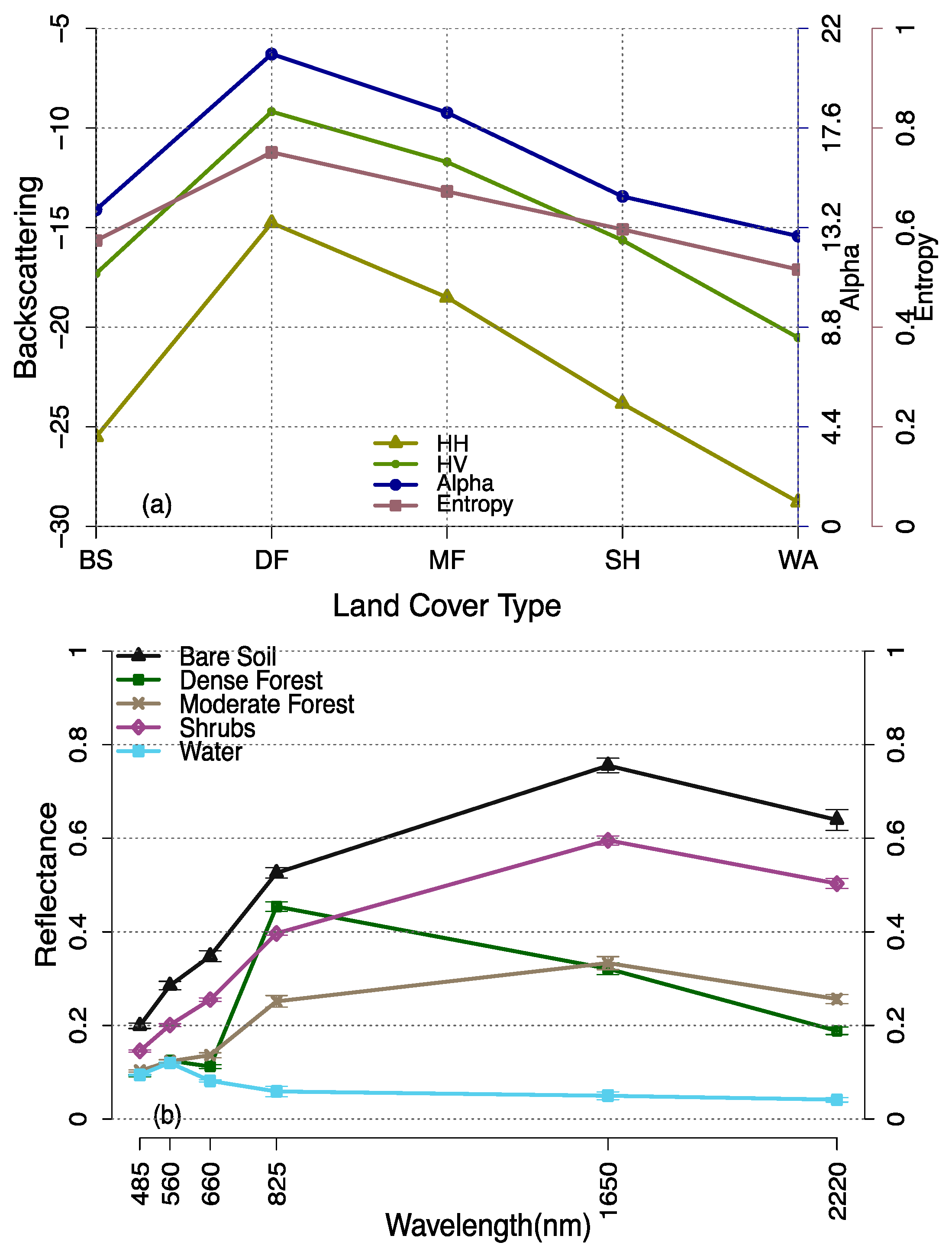
Figure 6.
(a,b) Cloude-Pottier decomposition of the training samples of the selected land cover classes (Table 1). Z1, Z4 and Z7 are characterized by double bounce scattering, Z3, Z6 and Z9 by surface scattering, and Z2, Z5 and Z8 by volume scattering. The black dashed polygon indicates the extent of Figure 5b; a zoomed view of the training samples distribution on the Alpha-Entropy plane.
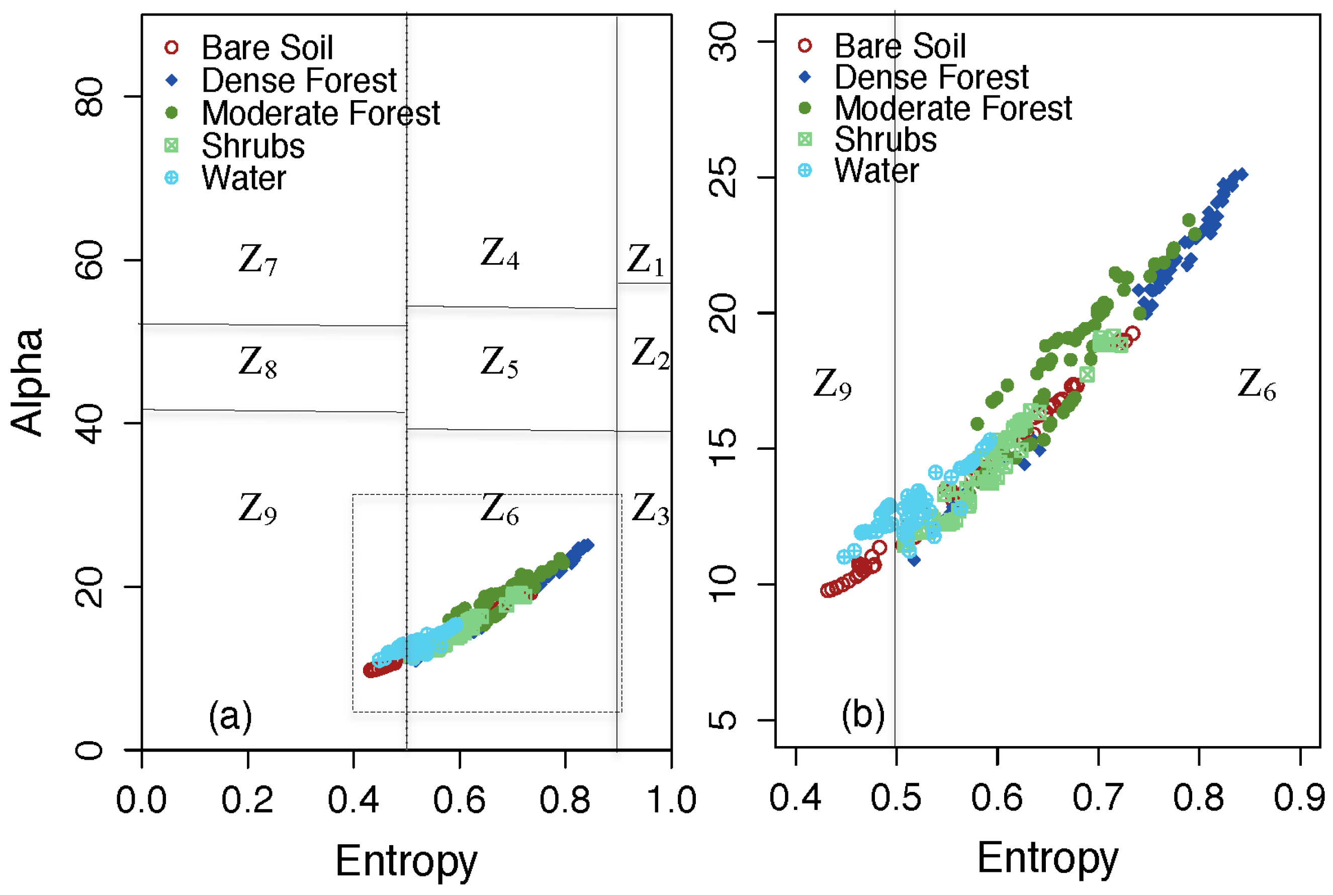
Figure 7.
Comparison of the overall classification accuracy achieved on different data categories based on the validation samples.
Figure 7.
Comparison of the overall classification accuracy achieved on different data categories based on the validation samples.

Figure 8.
Land cover map produces based on integration of Landsat TM and ALOS PALSAR data.


| Land Cover Type | Description |
|---|---|
| Water (WA) | This consist of Lake Babati and wetland areas |
| Shrubs (SH) | This is composed of bushed grasslands, bushed grasslands, which are seasonally inundated, and bush land with scattered cropland and trees |
| Moderate forest (MF) | This is a low density forest, composed of open woodland, closed woodland, wooded grasslands and woodland with scattered cropland |
| Dense forest (DF) | This is a dense forest comprised of forest that reproduce naturally, originating from the original forest cover |
| Bare soil (BS) | This is composed of bare land without grasses, shrubs or forests |
| Satellite/ Sensor | Bands | Acquisition Date |
|---|---|---|
| Landsat 5/TM | 1,2,3,4,5, 7 | 4 November 2009 |
| ALOS/PALSAR | L band | 13 September 2009 |
| Vegetation Indices | Description of Symbols | Reference | |
|---|---|---|---|
| Index Under Study | Formula | ||
| NDVI | (IR − R)/(IR + R) | Normalized Difference Vegetation Index (TM: 660 nm; 830 nm) | [17] |
| SAVI | Soil Adjusted Vegetation Index (TM:660nm; 830 nm) | [36] | |
| SLAVI | Specific Leaf Area Vegetation Index. (TM: 660 nm; 2220 nm) | [37] | |
| RFDI | (HH-HV)/(HH+HV) | Radar Forest Deforestation Index (Measure of different vegetation types cover) | [32] |
| PCA | |||
| PCA1 | 0.054TM1 + 0.130TM2 +0.143TM3 + 0.595TM4 +0.709TM5 + 0.321TM7 | Principal component analysis band 1 | [38,40] |
| PCA2 | −0.079TM1 − 0.121TM2 -0.212TM3 + 0.787TM4 − 0.421TM5 − 0.372TM7 | Principal component analysis band 2 | |
| PCA3 | 0.230TM1 + 0.504TM2 + 0.616TM3 + 0.140TM4 − 0.472TM5 + 0.266TM7 | Principal component analysis band 3 | |
| PCA4 | 0.054TM1 + 0.130TM2 + 0.143TM3 + 0.595TM4 + 0.709TM5 + 0.321TM7 | Principal component analysis band 4 | |
| PCA5 | −0.079TM1 − 0.121TM2 -0.212TM3 + 0.787TM4 − 0.421TM5 − 0.372TM7 | Principal component analysis band 5 | |
| PCA6 | 0.230TM1 + 0.504TM2 + 0.616TM3 + 0.140TM4 − 0.472TM5 + 0.266TM7 | Principal component analysis band 6 | |
| GLCM Textural Measures | |||
| Mean | Measure of textural features; p(i,j) is a normalized grey–tone spatial dependence matrix such that SUM (i,j = 0, N − 1) (P(i,j)) = 1; i and j represent row and column respectively. | ||
| Variance | Measure of textural features; μ is the mean | [34] | |
| Contrast | Measure of textural features, N is the number of distinct grey levels in the quantized image | ||
| Correlation | Measure of textural features; μx, μy, σx and σy are the means and standard deviations of px and py respectively | ||
| Dissimilarity | Measure of textural features | ||
| Entropy | Measure of textural features | ||
| Homogeneity | Measure of textural features | ||
| Angular second moment (ASM) | Measure of textural features | ||
Table 4.
Dataset categorization for various classification scenarios. PCA1 stands for the first component of PCA, mea: mean, cor: correlation, var: variance, con: contrast, and sec: second moment are co-occurrence matrix texture measures.
| Category | Datasets | Selected Input Data or Combination | |
|---|---|---|---|
| A | A1 | TM surface reflectance | TM bands (1,2,3,4,5,7) |
| A2 | TM derivatives (VI, PCA and GLCM texture) | PCA1, SLAVI, mea_b1, cor_b3, var_b4, cor_b4, con_b4 | |
| A3 | TM surface reflectance and TM derivatives | TM bands(123457), PCA1, SLAVI, cor_b3, var_b4, cor_b4, con_b4 | |
| B | B1 | PALSAR bands | HH, HV |
| B2 | PALSAR derivatives (RFDI, quotient bands, polarimetric features, and GLCM textures) | RFDI, HH/HV, HV/HH, HH-HV, alpha, entropy, cor_HH, cor_HV, mea_HH, var_HH, sec_HH, sec_HV | |
| B3 | PALSAR bands, RFDI and quotient bands | HH, RFDI, HH/HV, HV/HH, HH-HV | |
| B4 | PALSAR bands, PALSAR GLCM textures | HH, cor_HH, cor_HV, mea_HH, var_HH, se_HH, sec_HV | |
| B5 | PALSAR bands and Polarimetric features | HH, HV, alpha, entropy | |
| B6 | PALSAR bands and their derivatives | HH, HH/HV, HV/HH, alpha, entropy, cor_HH, cor_HV, mea_HH, var_HH, sec_HH, sec_HV | |
| C | C1 | TM surface reflectance, PALSAR bands | TM bands (1,2,3,4,5,7), HH, HV |
| C2 | TM derivatives and PALSAR Bands | PCA1, SLAVI, mea_b1, cor_b3, var_b4, cor_b4, con_b4, HH, HV | |
| C3 | TM derivatives and Polarimetric features | PCA1, SLAVI, mea_b1, cor_b3, var_b4, cor_b4, con_b4, alpha, entropy | |
| C4 | TM derivatives and GLCM textures of PALSAR bands | PCA1, SLAVI, mea_b1, cor_b3, var_b4, cor_b4, con_b4, cor_HH, cor_HV, mea_HH, var_HH, sec_HH, sec_HV | |
| C5 | TM and PALSAR derivatives | SLAVI, cor_b3, var_b4, cor_b4, con_b4, HH/HV, HV/HH, HH-HV, alpha, entropy, cor_HH, cor_HV, mea_HH, var_HH, sec_HH, sec_HV | |
| C6 | TM surface reflectance, PALSAR backscattering and their derivatives | TM bands(1,2,3,4,5,7), HH, HV, SLAVI, cor_b3, var_b4, cor_b4, con_b4, alpha, entropy, cor_HH, cor_HV, mea_HH, var_HH, sec_HH, sec_HV | |
Table 5.
Extracted mean values of ALOS PALSAR backscattering (HH, HV), alpha and entropy based on the training samples for the selected land cover classes (Table 1).
| Class | BS | DF | MF | SH | WA |
|---|---|---|---|---|---|
| HH ( | −25.51 | −14.76 | −18.51 | −23.84 | −28.78 |
| HV ( | −17.31 | −9.18 | −11.70 | −15.63 | −20.52 |
| Alpha () | 13.99 | 20.87 | 18.28 | 14.58 | 12.83 |
| Entropy (H) | 0.57 | 0.75 | 0.67 | 0.60 | 0.52 |
Table 6.
Training samples separability values for various land cover class pair for all classification scenarios (A–C) (Table 5) based on Jeffries-Matusita (J-M) sparability index. WA: Water, DF: Dense Forest, MF: Moderate Forest, SH: Shrubs, BS: Bare Soil. J-M separability index values ≥1.8 are in bold.
| Class Pair | Category | ||||||||||||||
|---|---|---|---|---|---|---|---|---|---|---|---|---|---|---|---|
| A | B | C | |||||||||||||
| A1 | A2 | A3 | B1 | B2 | B3 | B4 | B5 | B6 | C1 | C2 | C3 | C4 | C5 | C6 | |
| DF-MF | 1.91 | 1.92 | 1.99 | 0.67 | 1.45 | 1.04 | 0.91 | 1.32 | 1.61 | 1.95 | 1.94 | 1.95 | 1.96 | 1.98 | 2.00 |
| DF-SH | 2.00 | 2.00 | 2.00 | 1.95 | 2.00 | 1.99 | 1.97 | 1.99 | 2.00 | 2.00 | 2.00 | 2.00 | 2.00 | 2.00 | 2.00 |
| DF-WA | 2.00 | 2.00 | 2.00 | 1.99 | 2.00 | 2.00 | 2.00 | 2.00 | 2.00 | 2.00 | 2.00 | 2.00 | 2.00 | 2.00 | 2.00 |
| DF-BS | 2.00 | 2.00 | 2.00 | 1.96 | 2.00 | 2.00 | 1.97 | 1.98 | 2.00 | 2.00 | 2.00 | 2.00 | 2.00 | 2.00 | 2.00 |
| MF-SH | 1.96 | 1.99 | 2.00 | 0.78 | 1.80 | 1.74 | 2.00 | 1.67 | 1.91 | 1.98 | 1.99 | 1.99 | 2.00 | 1.99 | 2.00 |
| MF-BS | 1.98 | 1.99 | 2.00 | 1.06 | 1.84 | 1.88 | 1.42 | 1.56 | 1.92 | 1.99 | 1.99 | 2.00 | 2.00 | 2.00 | 2.00 |
| MF-WA | 2.00 | 2.00 | 2.00 | 1.61 | 1.99 | 1.97 | 1.93 | 1.98 | 2.00 | 2.00 | 2.00 | 2.00 | 2.00 | 2.00 | 2.00 |
| SH-BS | 1.95 | 1.83 | 1.99 | 0.34 | 1.57 | 1.46 | 0.79 | 1.31 | 1.76 | 1.98 | 1.94 | 1.96 | 1.96 | 1.99 | 2.00 |
| SH-WA | 2.00 | 2.00 | 2.00 | 1.27 | 2.00 | 1.92 | 1.84 | 1.99 | 2.00 | 2.00 | 2.00 | 2.00 | 2.00 | 2.00 | 2.00 |
| BS-WA | 2.00 | 2.00 | 2.00 | 0.67 | 1.99 | 1.77 | 1.74 | 1.96 | 1.99 | 2.00 | 2.00 | 2.00 | 2.00 | 2.00 | 2.00 |
Table 7.
Producer’s/user’s accuracy comparison of land cover classification results for different data categories used for various classification scenarios; See Table 1 and Table 6 for the description of land cover classes. Prod. Acc. and User. Acc. stands for the producer and user accuracy respectively. Results are based on the validation dataset.
| Class | Data Category | |||||||||||||||
|---|---|---|---|---|---|---|---|---|---|---|---|---|---|---|---|---|
| A1 | A2 | A3 | B1 | B2 | B3 | B4 | B5 | B6 | C1 | C2 | C3 | C4 | C5 | C6 | ||
| Prod. Acc. | DF | 100 | 96.3 | 96.3 | 48.2 | 55.6 | 3.7 | 25.9 | 66.7 | 48.2 | 100 | 100 | 100 | 96.3 | 96.3 | 96.3 |
| MF | 98.0 | 96.0 | 98.0 | 70.0 | 46.0 | 100 | 40.0 | 54.0 | 46.0 | 98.0 | 98.0 | 98.0 | 98.0 | 98.0 | 100 | |
| SH | 100 | 97.9 | 100 | 56.3 | 70.8 | 43.8 | 70.8 | 62.5 | 77.1 | 100 | 97.9 | 97.9 | 95.8 | 100 | 100 | |
| WA | 92.0 | 92.0 | 96.0 | 72.0 | 80.0 | 76.0 | 76.0 | 72.0 | 80.0 | 96.3 | 92.0 | 96.0 | 96.0 | 96.0 | 96.0 | |
| BS | 96.3 | 96.3 | 96.3 | 44.4 | 44.4 | 44.4 | 48.2 | 55.6 | 48.2 | 88.0 | 96.3 | 96.3 | 96.3 | 96.3 | 96.3 | |
| User. Acc. | DF | 100 | 100 | 100 | 48.2 | 34.9 | 100 | 18.4 | 42.9 | 31.7 | 100 | 100 | 100 | 100 | 100 | 100 |
| MF | 96.1 | 94.1 | 96.1 | 57.4 | 46.9 | 52.1 | 35.1 | 52.9 | 44.2 | 94.2 | 96.1 | 98.0 | 96.0 | 96.1 | 96.2 | |
| SH | 96.0 | 94.0 | 96.0 | 65.9 | 81.0 | 84.0 | 82.9 | 76.9 | 80.4 | 96.0 | 95.9 | 95.9 | 95.8 | 96.0 | 98.0 | |
| WA | 100 | 100 | 100 | 94.7 | 100 | 90.5 | 100 | 100 | 100 | 100 | 100 | 100 | 100 | 100 | 100 | |
| BS | 100 | 96.3 | 100 | 41.4 | 52.2 | 35.3 | 59.1 | 55.6 | 72.2 | 100 | 96.3 | 96.3 | 92.8 | 100 | 100 | |
| F1 Score | DF | 1.00 | 0.98 | 0.98 | 0.48 | 0.43 | 0.07 | 0.22 | 0.52 | 0.38 | 1.00 | 1.00 | 1.00 | 0.98 | 0.98 | 0.98 |
| MF | 0.97 | 0.95 | 0.97 | 0.63 | 0.46 | 0.68 | 0.37 | 0.53 | 0.45 | 0.96 | 0.97 | 0.98 | 0.97 | 0.97 | 0.98 | |
| SH | 0.98 | 0.96 | 0.98 | 0.61 | 0.76 | 0.58 | 0.76 | 0.69 | 0.79 | 0.98 | 0.97 | 0.97 | 0.96 | 0.98 | 0.99 | |
| WA | 0.96 | 0.96 | 0.98 | 0.82 | 0.89 | 0.83 | 0.86 | 0.84 | 0.89 | 0.98 | 0.96 | 0.98 | 0.98 | 0.98 | 0.98 | |
| BS | 0.98 | 0.96 | 0.98 | 0.43 | 0.48 | 0.39 | 0.53 | 0.56 | 0.58 | 0.94 | 0.96 | 0.96 | 0.95 | 0.98 | 0.98 | |
© 2016 by the author; licensee MDPI, Basel, Switzerland. This article is an open access article distributed under the terms and conditions of the Creative Commons Attribution (CC-BY) license (http://creativecommons.org/licenses/by/4.0/).
Share and Cite
MDPI and ACS Style
Deus, D. Integration of ALOS PALSAR and Landsat Data for Land Cover and Forest Mapping in Northern Tanzania. Land 2016, 5, 43. https://doi.org/10.3390/land5040043
AMA Style
Deus D. Integration of ALOS PALSAR and Landsat Data for Land Cover and Forest Mapping in Northern Tanzania. Land. 2016; 5(4):43. https://doi.org/10.3390/land5040043
Chicago/Turabian StyleDeus, Dorothea. 2016. "Integration of ALOS PALSAR and Landsat Data for Land Cover and Forest Mapping in Northern Tanzania" Land 5, no. 4: 43. https://doi.org/10.3390/land5040043
Note that from the first issue of 2016, this journal uses article numbers instead of page numbers. See further details here.