The Gradient Effect on the Relationship between the Underlying Factor and Land Surface Temperature in Large Urbanized Region

 , and
, and
Abstract
:1. Introduction
2. Methodology
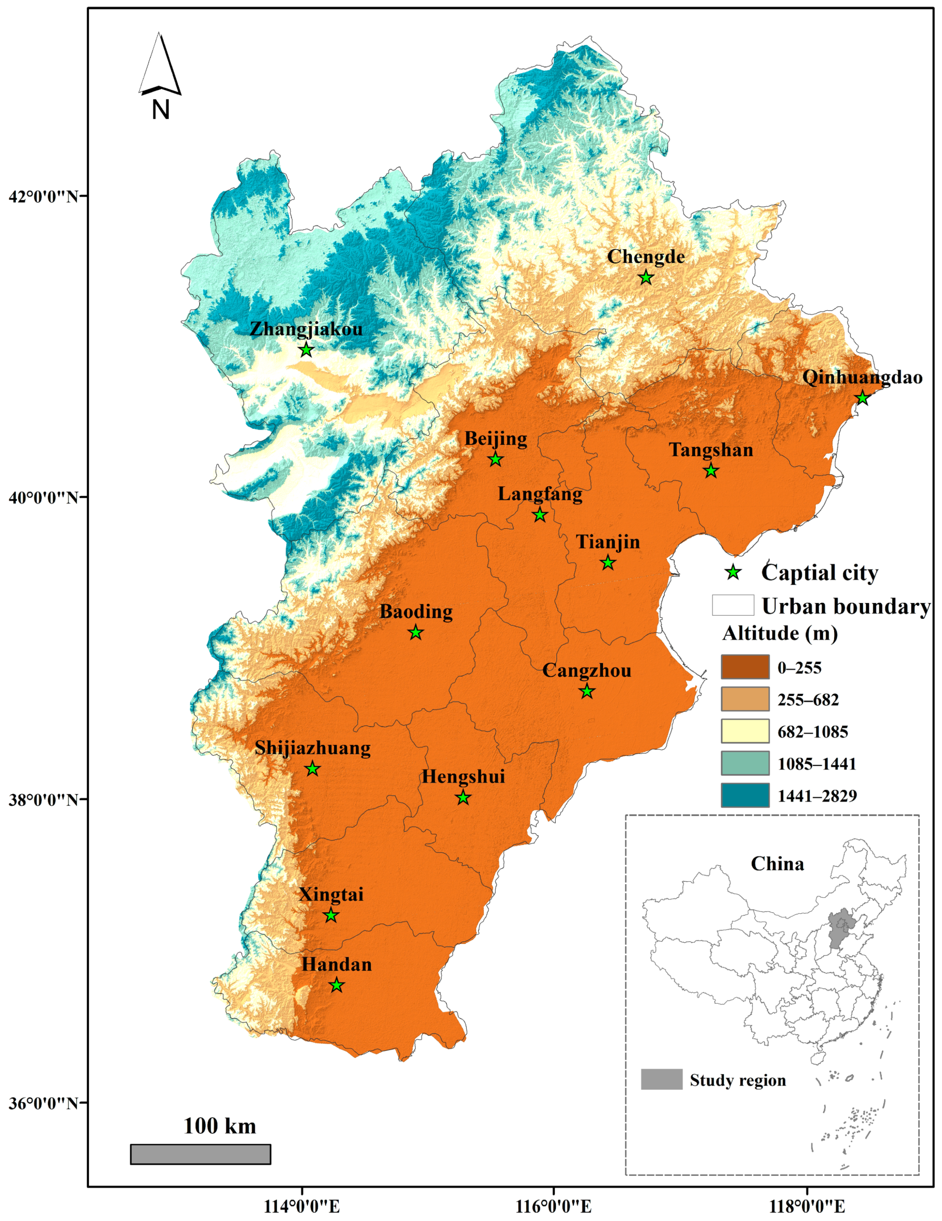
2.1. Study Area
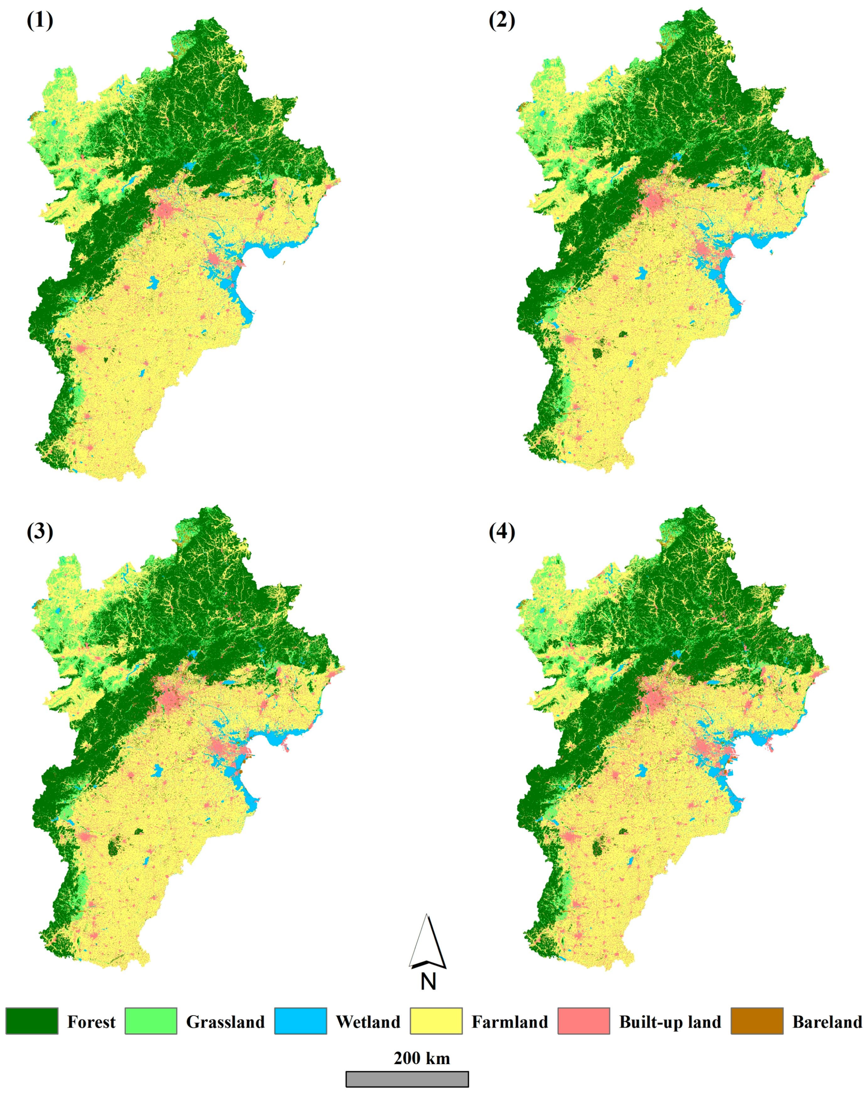
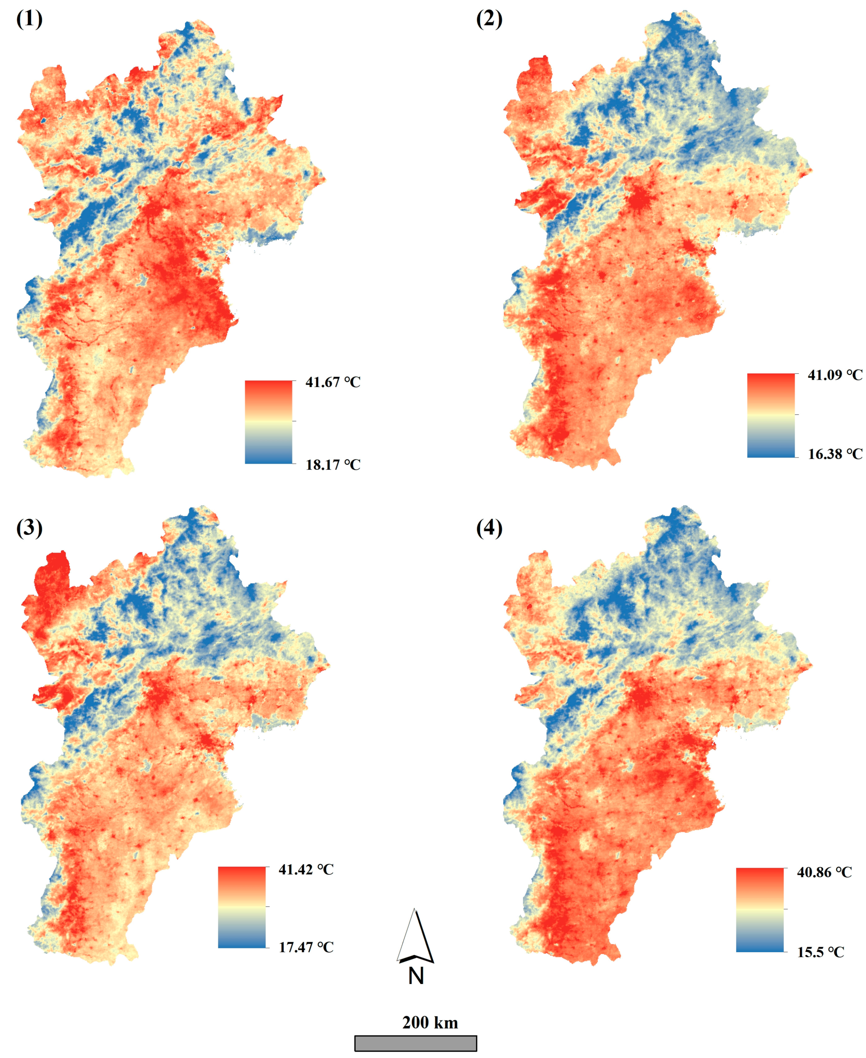
2.2. Land Cover and Land Surface Temperature Data
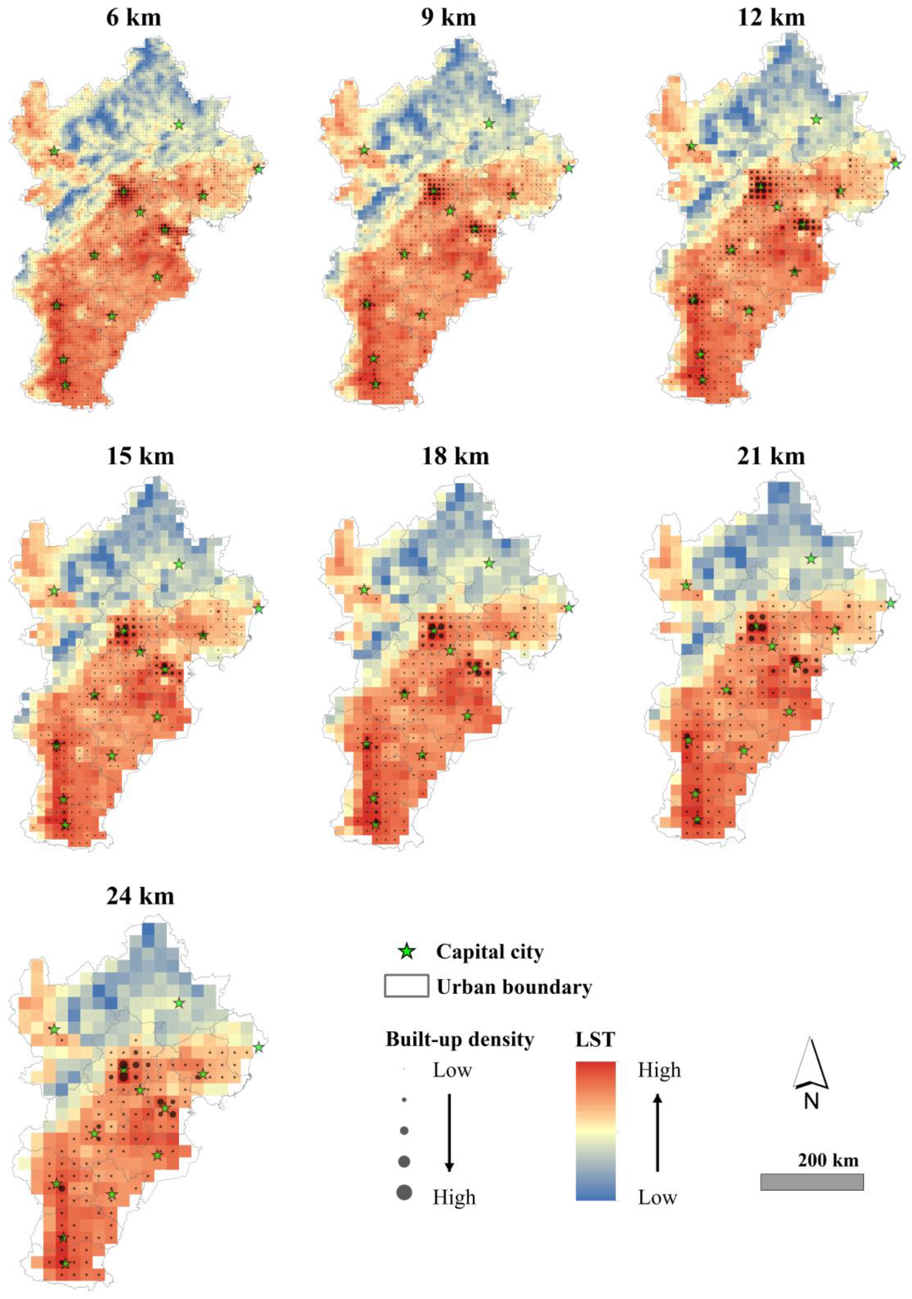
2.3. Grid Analysis Design
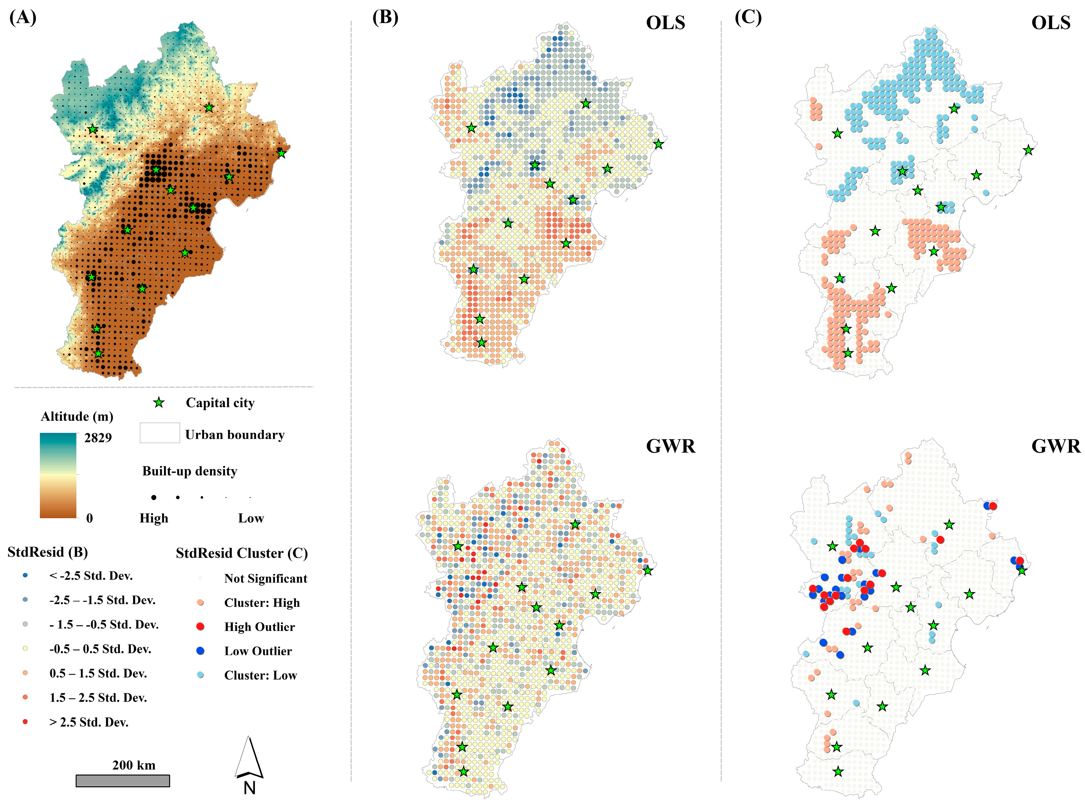
2.4. Statistical Analysis
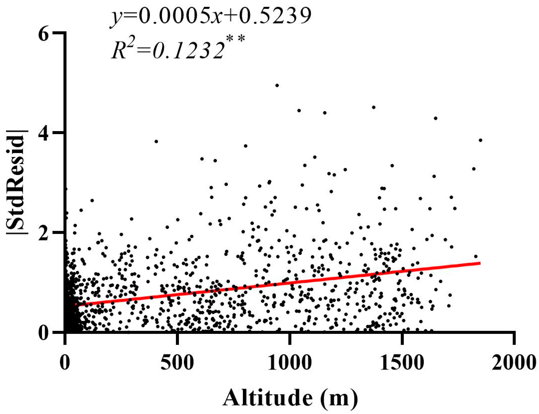
3. Results
4. Discussion
4.1. The Relationships between LST and the Built-Up Density Revealed by the OLS and GWR Models
4.2. Implications and Limitations of this Study
5. Conclusions
Author Contributions
Funding
Data Availability Statement
Acknowledgments
Conflicts of Interest
References
- Wu, Z.; Ren, Y. A bibliometric review of past trends and future prospects in urban heat island research from 1990 to 2017. Environ. Rev. 2019, 27, 241–251. [Google Scholar] [CrossRef]
- Arnfield, A.J. Two decades of urban climate research: A review of turbulence, exchanges of energy and water, and the urban heat island. Int. J. Clim. 2003, 23, 1–26. [Google Scholar] [CrossRef]
- Gago, E.J.; Roldan, J.; Pacheco-Torres, R.; Ordonez, J. The city and urban heat islands: A review of strategies to mitigate adverse effects. Renew. Sustain. Energy Rev. 2013, 25, 749–758. [Google Scholar] [CrossRef]
- Manoli, G.; Fatichi, S.; Bou-Zeid, E.; Katul, G.G. Seasonal hysteresis of surface urban heat islands. Proc. Natl. Acad. Sci. USA 2020, 117, 7082–7089. [Google Scholar] [CrossRef]
- Nastran, M.; Kobal, M.; Eler, K. Urban heat islands in relation to green land use in European cities. Urban For. Urban Green. 2019, 37, 33–41. [Google Scholar] [CrossRef] [Green Version]
- Deilami, K.; Kamruzzaman, M.; Liu, Y. Urban heat island effect: A systematic review of spatio-temporal factors, data, methods, and mitigation measures. Int. J. Appl. Earth Obs. Geoinf. 2018, 67, 30–42. [Google Scholar] [CrossRef]
- Chen, A.; Sun, R.; Chen, L. Studies on urban heat island from a landscape pattern view: A review. Acta Ecol. Sin. 2012, 32, 4553–4565. [Google Scholar] [CrossRef] [Green Version]
- Chen, A.; Yao, L.; Sun, R.; Li, J. How many metrics are required to identify the effects of the landscape pattern on land surface temperature? Ecol. Indic. 2014, 45, 424–433. [Google Scholar] [CrossRef]
- Kaufmann, R.K.; Seto, K.C.; Schneider, A.; Liu, Z.; Zhou, L.; Wang, W. Climate Response to Rapid Urban Growth: Evidence of a Human-Induced Precipitation Deficit. J. Clim. 2007, 20, 2299–2306. [Google Scholar] [CrossRef]
- Amanollahi, J.; Tzanis, C.G.; Ramli, M.; Abdullah, A.M. Urban heat evolution in a tropical area utilizing Landsat imagery. Atmos. Res. 2016, 167, 175–182. [Google Scholar] [CrossRef]
- Forman, R.; Godron, M. Landscape Ecology; John Wiley and Sons: New York, NY, USA, 1986. [Google Scholar]
- Zhao, C.; Jensen, J.L.R.; Weng, Q.; Weaver, R. A Geographically Weighted Regression Analysis of the Underlying Factors Related to the Surface Urban Heat Island Phenomenon. Remote Sens. 2018, 10, 1428. [Google Scholar] [CrossRef] [Green Version]
- Li, X.; Zhou, W. Spatial patterns and driving factors of surface urban heat island intensity: A comparative study for two agriculture-dominated regions in China and the USA. Sustain. Cities Soc. 2019, 48, 48. [Google Scholar] [CrossRef]
- Liang, Z.; Wu, S.; Wang, Y.; Wei, F.; Huang, J.; Shen, J.; Li, S. The relationship between urban form and heat island intensity along the urban development gradients. Sci. Total Environ. 2020, 708, 135011. [Google Scholar] [CrossRef] [PubMed]
- Grimm, N.B.; Foster, D.; Groffman, P.; Grove, J.M.; Hopkinson, C.S.; Nadelhoffer, K.J.; Pataki, D.E.; Peters, D.P. The changing landscape: Ecosystem responses to urbanization and pollution across climatic and societal gradients. Front. Ecol. Environ. 2008, 6, 264–272. [Google Scholar] [CrossRef] [Green Version]
- Yuan, S.; Xia, H.; Yang, L. How changing grain size affects the land surface temperature pattern in rapidly urbanizing area: A case study of the central urban districts of Hangzhou City, China. Environ. Sci. Pollut. Res. 2020, 1–15. [Google Scholar] [CrossRef] [PubMed]
- Peng, J.; Xie, P.; Liu, Y.; Ma, J. Urban thermal environment dynamics and associated landscape pattern factors: A case study in the Beijing metropolitan region. Remote Sens. Environ. 2016, 173, 145–155. [Google Scholar] [CrossRef]
- Zhou, W.; Qian, Y.; Li, X.; Li, W.; Han, L. Relationships between land cover and the surface urban heat island: Seasonal variability and effects of spatial and thematic resolution of land cover data on predicting land surface temperatures. Landsc. Ecol. 2014, 29, 153–167. [Google Scholar] [CrossRef]
- Yao, L.; Xu, Y.; Zhang, B. Effect of urban function and landscape structure on the urban heat island phenomenon in Beijing, China. Landsc. Ecol. Eng. 2019, 15, 379–390. [Google Scholar] [CrossRef]
- Deilami, K.; Kamruzzaman, M.; Hayes, J.F. Correlation or Causality between Land Cover Patterns and the Urban Heat Island Effect? Evidence from Brisbane, Australia. Remote Sens. 2016, 8, 716. [Google Scholar] [CrossRef] [Green Version]
- National Bureau of Statistics. China City Statistical Yearbook; China Statistical Press: Beijing, China, 2015.
- Li, X.; Kuang, W. Spatio-Temporal Trajectories of Urban Land Use Change during 1980–2015 and Future Scenario Simulation in Beijing-Tianjin-Hebei Urban Agglomeration. Econ. Geogr. 2019, 39, 187–194, 200. [Google Scholar] [CrossRef]
- Zhao, N.; Jiao, Y.; Ma, T.; Zhao, M.; Fan, Z.; Yin, X.; Liu, Y.; Yue, T. Estimating the effect of urbanization on extreme climate events in the Beijing-Tianjin-Hebei region, China. Sci. Total Environ. 2019, 688, 1005–1015. [Google Scholar] [CrossRef] [PubMed]
- Kang, S.; Eltahir, E.A.B. North China Plain threatened by deadly heatwaves due to climate change and irrigation. Nat. Commun. 2018, 9, 1–9. [Google Scholar] [CrossRef] [Green Version]
- Wang, D.; Sang, M.; Huang, Y.; Chen, L.; Wei, X.; Chen, W.; Wang, F.; Liu, J.; Hu, B. Trajectory analysis of agricultural lands occupation and its decoupling relationships with the growth rate of non-agricultural GDP in the Jing-Jin-Tang region, China. Environ. Dev. Sustain. 2018, 21, 799–815. [Google Scholar] [CrossRef]
- Yu, W.; Zhou, W.; Qian, Y.; Yan, J. A new approach for land cover classification and change analysis: Integrating backdating and an object-based method. Remote Sens. Environ. 2016, 177, 37–47. [Google Scholar] [CrossRef]
- Wan, Z.; Zhang, Y.; Zhang, Q.; Li, Z.-L. Validation of the land-surface temperature products retrieved from Terra Moderate Resolution Imaging Spectroradiometer data. Remote Sens. Environ. 2002, 83, 163–180. [Google Scholar] [CrossRef]
- Rigo, G.; Parlow, E.; Oesch, D. Validation of satellite observed thermal emission with in-situ measurements over an urban surface. Remote Sens. Environ. 2006, 104, 201–210. [Google Scholar] [CrossRef]
- Zhou, D.; Zhao, S.; Zhang, L.; Sun, G.; Liu, Y. The footprint of urban heat island effect in China. Sci. Rep. 2015, 5, 11160. [Google Scholar] [CrossRef]
- Liu, F.; Zhang, X.; Murayama, Y.; Morimoto, T. Impacts of Land Cover/Use on the Urban Thermal Environment: A Comparative Study of 10 Megacities in China. Remote Sens. 2020, 12, 307. [Google Scholar] [CrossRef] [Green Version]
- Zhou, D.; Zhang, L.; Li, D.; Huang, D.; Zhu, C. Climate–vegetation control on the diurnal and seasonal variations of surface urban heat islands in China. Environ. Res. Lett. 2016, 11, 074009. [Google Scholar] [CrossRef]
- Wu, J. Effects of changing scale on landscape pattern analysis: Scaling relations. Landsc. Ecol. 2004, 19, 125–138. [Google Scholar] [CrossRef]
- Zhang, Q.; Wu, Z.; Zhang, H.; Fontana, G.D.; Tarolli, P. Identifying dominant factors of waterlogging events in metropolitan coastal cities: The case study of Guangzhou, China. J. Environ. Manag. 2020, 271, 110951. [Google Scholar] [CrossRef]
- Cadenasso, M.L.; Pickett, S.T.A.; Schwarz, K. Spatial heterogeneity in urban ecosystems: Reconceptualizing land cover and a framework for classification. Front. Ecol. Environ. 2007, 5, 80–88. [Google Scholar] [CrossRef]
- Li, X.; Zhou, W. Optimizing urban greenspace spatial pattern to mitigate urban heat island effects: Extending understanding from local to the city scale. Urban For. Urban Green. 2019, 41, 255–263. [Google Scholar] [CrossRef]
- Yao, L.; Li, T.; Xu, M.; Xu, Y. How the landscape features of urban green space impact seasonal land surface temperatures at a city-block-scale: An urban heat island study in Beijing, China. Urban For. Urban Green. 2020, 52, 126704. [Google Scholar] [CrossRef]
- Zhou, W.; Huang, G.; Cadenasso, M.L. Does spatial configuration matter? Understanding the effects of land cover pattern on land surface temperature in urban landscapes. Landsc. Urban Plan. 2011, 102, 54–63. [Google Scholar] [CrossRef]
- Hou, H.; Estoque, R.C. Detecting Cooling Effect of Landscape from Composition and Configuration: An Urban Heat Island Study on Hangzhou. Urban For. Urban Green. 2020, 53, 126719. [Google Scholar] [CrossRef]
- Imhoff, M.L.; Zhang, P.; Wolfe, R.E.; Bounoua, L. Remote sensing of the urban heat island effect across biomes in the continental USA. Remote Sens. Environ. 2010, 114, 504–513. [Google Scholar] [CrossRef] [Green Version]
- Meng, Q.; Zhang, L.; Sun, Z.; Meng, F.; Wang, L.; Sun, Y. Characterizing spatial and temporal trends of surface urban heat island effect in an urban main built-up area: A 12-year case study in Beijing, China. Remote Sens. Environ. 2018, 204, 826–837. [Google Scholar] [CrossRef]
- Peng, J.; Jiansheng, W.; Liu, Y.; Li, H.; Wu, J. Seasonal contrast of the dominant factors for spatial distribution of land surface temperature in urban areas. Remote Sens. Environ. 2018, 215, 255–267. [Google Scholar] [CrossRef]
- Sun, R.; Lü, Y.; Li, J.; Yang, L.; Chen, A. Assessing the stability of annual temperatures for different urban functional zones. Build. Environ. 2013, 65, 90–98. [Google Scholar] [CrossRef]
- Buyantuyev, A.; Wu, J. Urban heat islands and landscape heterogeneity: Linking spatiotemporal variations in surface temperatures to land-cover and socioeconomic patterns. Landsc. Ecol. 2010, 25, 17–33. [Google Scholar] [CrossRef]
- Zhang, L.; Gove, J.H.; Heath, L.S. Spatial residual analysis of six modeling techniques. Ecol. Model. 2005, 186, 154–177. [Google Scholar] [CrossRef]
- Wang, X.; Zhou, T.; Tao, F.; Zang, F. Correlation Analysis between UBD and LST in Hefei, China, Using Luojia1-01 Night-Time Light Imagery. Appl. Sci. 2019, 9, 5224. [Google Scholar] [CrossRef] [Green Version]
- Mitchel, A. The ESRI Guide to GIS Analysis, Volume 2: Spatial Measurements and Statistics; Esri Press: Redlands, CA, USA, 2005. [Google Scholar]
- Sun, R.; Xie, W.; Li, J. A landscape connectivity model to quantify contributions of heat sources and sinks in urban regions. Landsc. Urban Plan. 2018, 178, 43–50. [Google Scholar] [CrossRef]
- Wu, Z.; Yao, L.; Ren, Y. Characterizing the spatial heterogeneity and controlling factors of land surface temperature clusters: A case study in Beijing. Build. Environ. 2020, 169, 106598. [Google Scholar] [CrossRef]
- Stewart Fotheringham, A.; Charlton, M.; Brunsdon, C. The geography of parameter space: An investigation of spatial non-stationarity. Int. J. Geogr. Inf. Syst. 1996, 10, 605–627. [Google Scholar] [CrossRef]
- Weng, Q.; Lu, D.; Schubring, J. Estimation of land surface temperature–vegetation abundance relationship for urban heat island studies. Remote Sens. Environ. 2004, 89, 467–483. [Google Scholar] [CrossRef]
- Zhang, X.; Zhou, J.; Liang, S.; Chai, L.; Wang, D.; Liu, J. Estimation of 1-km all-weather remotely sensed land surface temperature based on reconstructed spatial-seamless satellite passive microwave brightness temperature and thermal infrared data. ISPRS J. Photogramm. Remote Sens. 2020, 167, 321–344. [Google Scholar] [CrossRef]
- Yoo, C.; Im, J.; Cho, D.; Yokoya, N.; Xia, J.; Bechtel, B. Estimation of All-Weather 1 km MODIS Land Surface Temperature for Humid Summer Days. Remote Sens. 2020, 12, 1398. [Google Scholar] [CrossRef]
- Venter, Z.S.; Brousse, O.; Esau, I.; Meier, F. Hyperlocal mapping of urban air temperature using remote sensing and crowdsourced weather data. Remote Sens. Environ. 2020, 242, 111791. [Google Scholar] [CrossRef]
- Liu, Y.; Peng, J.; Wang, Y. Efficiency of landscape metrics characterizing urban land surface temperature. Landsc. Urban Plan. 2018, 180, 36–53. [Google Scholar] [CrossRef]
- Qiao, Z.; Wu, C.; Zhao, D.; Xu, X.; Yang, J.; Li, F.; Sun, Z.; Liu, L. Determining the Boundary and Probability of Surface Urban Heat Island Footprint Based on a Logistic Model. Remote Sens. 2019, 11, 1368. [Google Scholar] [CrossRef] [Green Version]
- Chen, A.; Yao, X.A.; Sun, R.; Chen, L. Effect of urban green patterns on surface urban cool islands and its seasonal variations. Urban For. Urban Green. 2014, 13, 646–654. [Google Scholar] [CrossRef]


| Forest | Grassland | Wetland | Farmland | Built-Up Land | Bareland | |
|---|---|---|---|---|---|---|
| 2000 | 70.27 | 18.82 | 6.35 | 101.60 | 17.86 | 0.63 |
| 2005 | 71.10 | 19.72 | 6.21 | 98.44 | 19.52 | 0.58 |
| 2010 | 71.56 | 19.94 | 6.00 | 95.98 | 21.64 | 0.70 |
| 2015 | 70.75 | 19.01 | 5.93 | 93.52 | 25.97 | 0.65 |
| 6 km | 9 km | 12 km | 15 km | 18 km | 21 km | 24 km | |
|---|---|---|---|---|---|---|---|
| Year | Forest | ||||||
| 2000 | −0.50 ** | −0.52 ** | −0.53 ** | −0.55 ** | −0.58 ** | −0.57 ** | −0.57 ** |
| 2005 | −0.65 ** | −0.66 ** | −0.66 ** | −0.66 ** | −0.68 ** | −0.67 ** | −0.68 ** |
| 2010 | −0.71 ** | −0.72 ** | −0.71 ** | −0.73 ** | −0.74 ** | −0.73 ** | −0.74 ** |
| 2015 | −0.71 ** | −0.72 ** | −0.73 ** | −0.74 ** | −0.76 | −0.76 ** | −0.77 ** |
| Grassland | |||||||
| 2000 | −0.10 ** | −0.16 ** | −0.19 ** | −0.21 ** | −0.25 ** | −0.28 ** | −0.26 ** |
| 2005 | −0.16 ** | −0.19 ** | −0.20 ** | −0.20 ** | −0.22 ** | −0.25 ** | −0.22 ** |
| 2010 | −0.06 ** | −0.09 ** | −0.09 ** | −0.10 ** | −0.11 ** | −0.15 ** | −0.13 * |
| 2015 | −0.34 ** | −0.38 ** | −0.39 ** | −0.39 ** | −0.40 ** | −0.42 ** | −0.43 ** |
| Wetland | |||||||
| 2000 | 0.38 ** | 0.39 ** | 0.40 ** | 0.42 ** | 0.44 ** | 0.42 ** | 0.37 ** |
| 2005 | 0.30 ** | 0.28 ** | 0.28 ** | 0.28 ** | 0.29 ** | 0.27 ** | 0.24 ** |
| 2010 | 0.33 ** | 0.33 ** | 0.33 ** | 0.35 ** | 0.35 ** | 0.33 ** | 0.30 ** |
| 2015 | 0.37 ** | 0.36 ** | 0.36 ** | 0.36 ** | 0.37 ** | 0.35 ** | 0.33 ** |
| Farmland | |||||||
| 2000 | 0.49 ** | 0.52 ** | 0.53 ** | 0.55 ** | 0.58 ** | 0.59 ** | 0.58 ** |
| 2005 | 0.56 ** | 0.58 ** | 0.59 ** | 0.60 ** | 0.63 ** | 0.63 ** | 0.63 ** |
| 2010 | 0.56 ** | 0.58 ** | 0.59 ** | 0.61 ** | 0.64 ** | 0.64 ** | 0.64 ** |
| 2015 | 0.61 ** | 0.63 ** | 0.65 ** | 0.66 ** | 0.68 ** | 0.68 ** | 0.70 ** |
| Built−up land | |||||||
| 2000 | 0.54 ** | 0.56 ** | 0.58 ** | 0.59 ** | 0.62 ** | 0.62 ** | 0.61 ** |
| 2005 | 0.65 ** | 0.65 ** | 0.66 ** | 0.66 ** | 0.67 ** | 0.66 ** | 0.65 ** |
| 2010 | 0.68 ** | 0.70 ** | 0.70 ** | 0.70 ** | 0.72 ** | 0.73 ** | 0.71 ** |
| 2015 | 0.79 ** | 0.80 ** | 0.81 ** | 0.82 ** | 0.83 ** | 0.82 ** | 0.83 ** |
| Bareland | |||||||
| 2000 | 0.04 ** | −0.14 ** | −0.15 ** | −0.14 ** | −0.16 ** | −0.17 ** | −0.14 * |
| 2005 | 0 | −0.21 ** | −0.22 ** | −0.22 ** | −0.22 ** | −0.23 ** | −0.16 ** |
| 2010 | 0.03 * | −0.12 ** | −0.11 ** | −0.08 * | −0.08 | −0.08 | −0.02 |
| 2015 | −0.04 * | −0.23 ** | −0.24 ** | −0.21 ** | −0.21 ** | −0.19 ** | −0.18 ** |
| 2000 | 2005 | |||||||||||
| OLS | GWR | OLS | GWR | |||||||||
| R2 | AICc | I | R2 | AICc | I | R2 | AICc | I | R2 | AICc | I | |
| 6 km | 0.17 | 24479.17 | 0.77 ** | 0.87 | 15270.01 | 0.14 ** | 0.27 | 24862.14 | 0.86 ** | 0.94 | 12315.42 | 0.09 ** |
| 9 km | 0.19 | 10476.87 | 0.76 ** | 0.88 | 7059.24 | 0.06 ** | 0.29 | 10733.62 | 0.85 ** | 0.94 | 6013.16 | 0.02 |
| 12 km | 0.21 | 5691.60 | 0.73 ** | 0.82 | 4038.76 | 0.12 ** | 0.31 | 5872.62 | 0.83 ** | 0.92 | 3462.75 | 0.00 |
| 15 km | 0.23 | 3533.23 | 0.68 ** | 0.83 | 2722.49 | 0.01 | 0.31 | 3672.54 | 0.81 ** | 0.92 | 2234.09 | 0.03 |
| 18 km | 0.25 | 2356.31 | 0.65 ** | 0.83 | 1870.14 | −0.01 | 0.33 | 2478.83 | 0.78 ** | 0.92 | 1500.88 | 0.00 |
| 21 km | 0.26 | 1685.72 | 0.61 ** | 0.79 | 1283.56 | 0.04 | 0.34 | 1767.62 | 0.75 ** | 0.92 | 1113.38 | −0.04 |
| 24 km | 0.28 | 1243.35 | 0.58 ** | 0.81 | 987.34 | −0.05 | 0.35 | 1323.79 | 0.74 ** | 0.91 | 836.45 | −0.06 |
| 2010 | 2015 | |||||||||||
| OLS | GWR | OLS | GWR | |||||||||
| R2 | AICc | I | R2 | AICc | I | R2 | AICc | I | R2 | AICc | I | |
| 6 km | 0.27 | 23948.98 | 0.81 ** | 0.93 | 12600.87 | 0.09 ** | 0.40 | 25968.57 | 0.81 ** | 0.95 | 13286.12 | 0.10 ** |
| 9 km | 0.30 | 10282.87 | 0.81 ** | 0.93 | 6399.90 | 0.00 | 0.43 | 11150.27 | 0.80 ** | 0.95 | 6485.29 | 0.04 ** |
| 12 km | 0.32 | 5596.47 | 0.76 ** | 0.90 | 3570.68 | 0.01 | 0.46 | 6078.48 | 0.78 ** | 0.94 | 3720.80 | 0.03 |
| 15 km | 0.33 | 3496.02 | 0.73 ** | 0.90 | 2355.67 | 0.01 | 0.48 | 53784.66 | 0.75 ** | 0.94 | 2616.84 | 0.02 |
| 18 km | 0.35 | 2346.47 | 0.69 ** | 0.89 | 1585.35 | 0.01 | 0.51 | 2544.73 | 0.73 ** | 0.94 | 1783.82 | 0.00 |
| 21 km | 0.38 | 1651.19 | 0.65 ** | 0.87 | 1159.82 | 0.03 | 0.52 | 1818.62 | 0.70 ** | 0.90 | 1231.49 | 0.14 ** |
| 24 km | 0.37 | 1241.42 | 0.62 ** | 0.88 | 895.61 | −0.04 | 0.54 | 1344.45 | 0.68 ** | 0.92 | 932.27 | −0.03 |
Publisher’s Note: MDPI stays neutral with regard to jurisdictional claims in published maps and institutional affiliations. |
© 2020 by the authors. Licensee MDPI, Basel, Switzerland. This article is an open access article distributed under the terms and conditions of the Creative Commons Attribution (CC BY) license (http://creativecommons.org/licenses/by/4.0/).
Share and Cite
Wang, Y.; Xu, M.; Li, J.; Jiang, N.; Wang, D.; Yao, L.; Xu, Y. The Gradient Effect on the Relationship between the Underlying Factor and Land Surface Temperature in Large Urbanized Region. Land 2021, 10, 20. https://doi.org/10.3390/land10010020
Wang Y, Xu M, Li J, Jiang N, Wang D, Yao L, Xu Y. The Gradient Effect on the Relationship between the Underlying Factor and Land Surface Temperature in Large Urbanized Region. Land. 2021; 10(1):20. https://doi.org/10.3390/land10010020
Chicago/Turabian StyleWang, Yixu, Mingxue Xu, Jun Li, Nan Jiang, Dongchuan Wang, Lei Yao, and Ying Xu. 2021. "The Gradient Effect on the Relationship between the Underlying Factor and Land Surface Temperature in Large Urbanized Region" Land 10, no. 1: 20. https://doi.org/10.3390/land10010020
APA StyleWang, Y., Xu, M., Li, J., Jiang, N., Wang, D., Yao, L., & Xu, Y. (2021). The Gradient Effect on the Relationship between the Underlying Factor and Land Surface Temperature in Large Urbanized Region. Land, 10(1), 20. https://doi.org/10.3390/land10010020