In this paper, we study the forecasting time of the invariant fuzzy time series of groundwater levels. The fuzzy C-mean algorithm is used for the fuzzification of the observed data, while the SSA is applied to make a forecasting model.
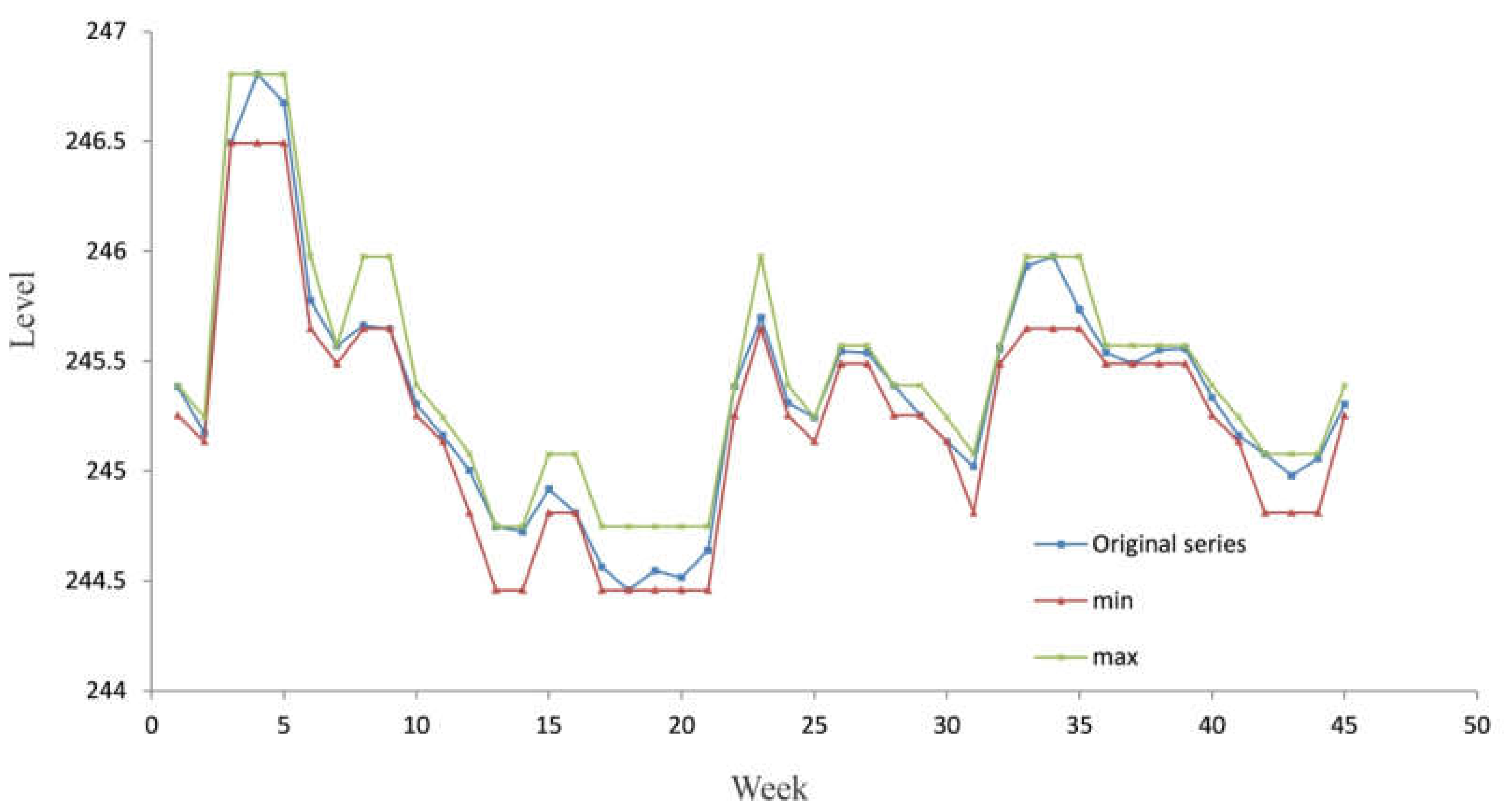
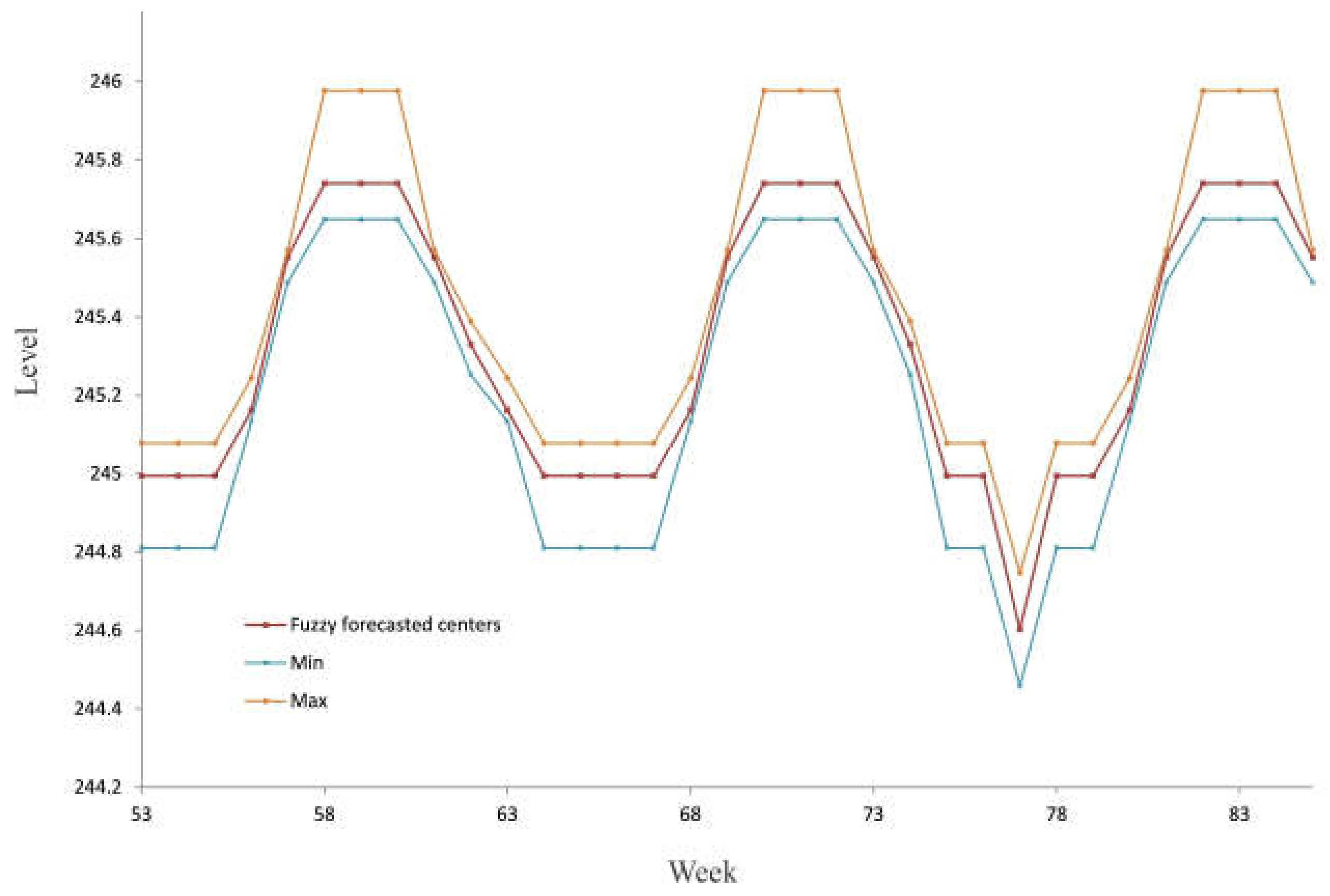
By applying linear recurrent formulae, we predict the future values of cluster centers. After that, the sequence of the forecasted cluster centers is transformed into a sequence of the actual centers obtained by fuzzy C-mean clustering. The transformation uses the equation of the fuzzy C-mean clustering algorithm, which calculates the membership degree. Finally, the developed model produces the interval time series, characterized by the minimum and maximum value of the groundwater level for every point in the future.
The developed model was tested by using the real data obtained by monitoring the groundwater source Perminac. It is located in the upstream area of Čačak city. The groundwater source contains 14 wells with a maximum total capacity of 131 l/s and an average of 90 l/s. In recent years, overexploitation caused a significant decrease in the groundwater level in the wider area of the groundwater source. Accordingly, some wells were excluded from the exploitation, and supply restrictions were introduced as a way of stabilizing consumption during the summer months.
2.1. Fuzzy Time Series
Song and Chissom [
18] first introduced the definition of fuzzy time series as follows [
19]:
“Let be the universe of observed data on which fuzzy sets are defined and let be a collection of . Then, is called a fuzzy time series on .”
Song and Chissom [
18] defined fuzzy relations among fuzzy time series, which are based on the assumption that the values of fuzzy time series
are fuzzy sets, and the observation of time
t is caused by the observations of the previous times [
19].
If for any
, there exist
and a fuzzy relation
such that
, where ”
” is the relation, then
is said to be caused by
only. It is expressed as follows:
Suppose that
is caused by
only, or by
or
or
. This relation can be expressed as follows:
Equation (2) represents the first-order model of . If is caused by
simultaneously, then their relations are represented as:
Equation (3) represents the k-th order model of , and is a relation matrix describing the fuzzy relationship between and .
To fuzzify the observed data, we apply the fuzzy C-mean algorithm.
2.2. A Brief Description of the Fuzzy C-mean Algorithm
In order to divide the observed data into an adequate number of fuzzy states, we apply the fuzzy C-mean clustering algorithm [
20,
21,
22,
23] over the set
. The reason that we clustered the time series is primarily related to the need to develop models that use the results of monitoring in a form that represents the states of the observed appearance. Decision-making models based on the interval inputs are much more flexible than deterministic models. Management models have a much higher confidence because they incorporate uncertainties expressed by intervals into management systems.
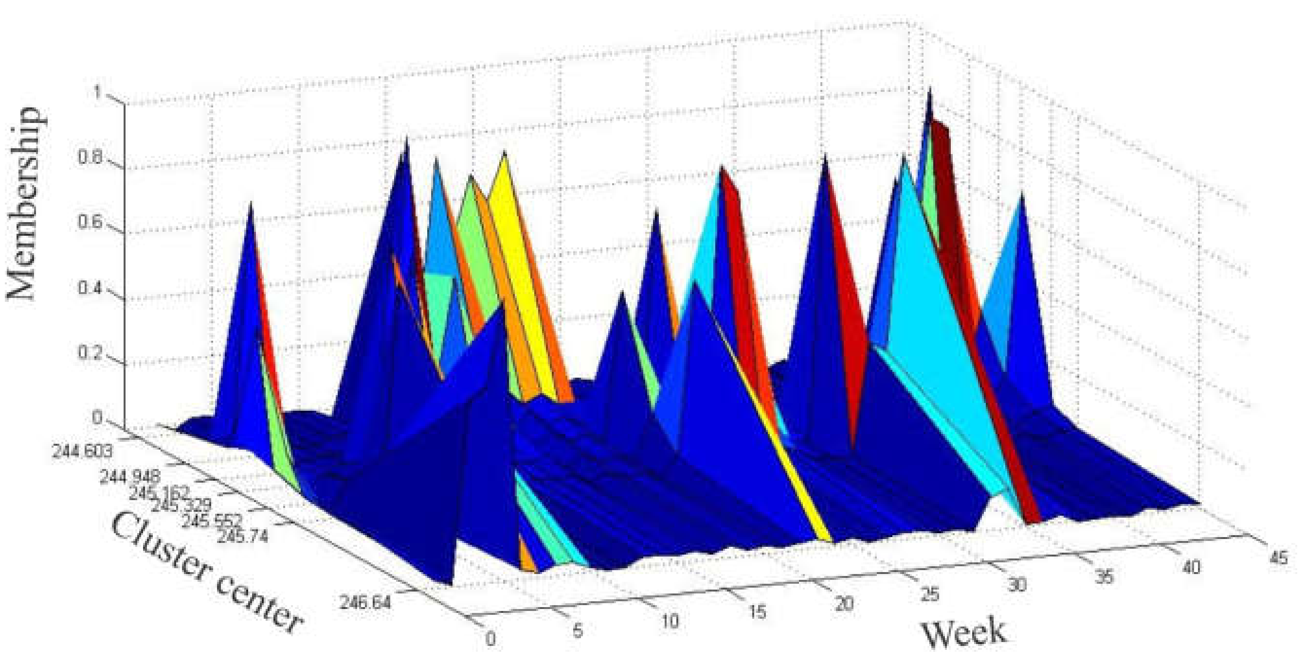
The fuzzy C-mean algorithm is a method based on the minimization of a generalized least-squared errors-function. Given a set , where N is the number of the observed data and q is the dimension of the sample . Every cluster is a fuzzy set defined by the relative closeness of space S. Suppose that there is a groundwater level vector composed of M cluster centers; . For the i-th relative closeness and m-th cluster center, there is a membership degree indicating with what degree the relative closeness SN belongs to the cluster center vector Cm, which results in a fuzzy partition matrix .
Let
uim be the membership,
cm the center of the cluster,
N the number of observed data and
M the number of clusters. This algorithm aims to determine cluster centers and the fuzzy partition matrix by minimizing the following function:
subject to
where
dim is Euclidean distance between the observation and the center of the cluster, defined as:
Finally, the objective function is:
The objective function
J represents the intra-cluster variance. If we want to have those elements that are most similar to the cluster center in a given cluster, we can do this by minimizing the variance inside the cluster. The exponent
ω is used to adjust the weighting effect of membership values. A large
ω will increase the fuzziness of the function
J. Pal and Bezdek [
24] suggested that
ω in the interval [1.5, 2.5] was generally recommended for use in FCM.
In this paper, the value of
ω is set to 2 as a midpoint of the suggested interval. The objective function is iteratively minimized. In
j-th iteration, the values of
and
are updated as follows:
The iteration process stops at , where represents the minimum amount of improvement. Sorting the sequence of obtained centers in an ascending order gives us .
The fuzzification of the data is done according to the results of the final fuzzy partition matrix.
The number of fuzzy sets corresponds to the number of clusters. Each row of the matrix
U represents the fuzzy state of that observation. Accordingly, we obtain the fuzzy state matrix of the observed data:
The state of the observed data is defined as:
Finally, the sequence Aim represents a fuzzy time series on . In this way, we obtain the transitions from one state to another over the time of observation; .
The creation of a set of certain transition rules for fuzzy relationships between states can be very difficult. To overcome this situation, we transform the fuzzy time series into an adequate time series of the center of the clusters. This approach enables us to apply a deterministic forecasting model based on the singular spectrum analysis.
2.3. Forecasting Model Based on the Singular Spectrum Analysis
The process of the transformation of the fuzzy time series into a crisp time series is based on the fact that each fuzzy state can be represented by a corresponding center of the cluster. Accordingly, the following time series, , are obtained.
The forecasting algorithm is based on SSA methodology [
25,
26,
27]. In SSA terminology, it is often assumed that the series is noisy with an arbitrary series length
N. The SSA technique consists of two main complementary stages: decomposition and reconstruction. The noisy series is decomposed in the first stage, and the noisy reduced series is reconstructed at the second stage. The reconstructed series will be used for forecasting the future values.
Consider the stochastic process and suppose that a realization of size N from this process is available: . Since we are faced with time-invariant series, and for simplicity, we can rewrite the realization as follows: .
The first stage of the algorithm, called decomposition, includes the following two steps: embedding and singular value decomposition (SVD).
Embedding is a mapping that transfers a one-dimensional time series of centers
into a multidimensional matrix
with vectors
, where
is the window length and
. The window length represents a vector of
L observations of the original series. If we remember Equation (3), we can see the window length model is similar to the
k-th order model of the fuzzy time series, but taking into account original values from
t = 1 to
t =
L. The usual value of
L is (
N + 1)/2 if
N is odd and
N/2 or (
N/2) + 1 if
N is even (for more details see [
27]). The result of this step is the trajectory matrix:
The trajectory matrix Y is the Hankel matrix where all elements along the diagonal i + j = const are equal.
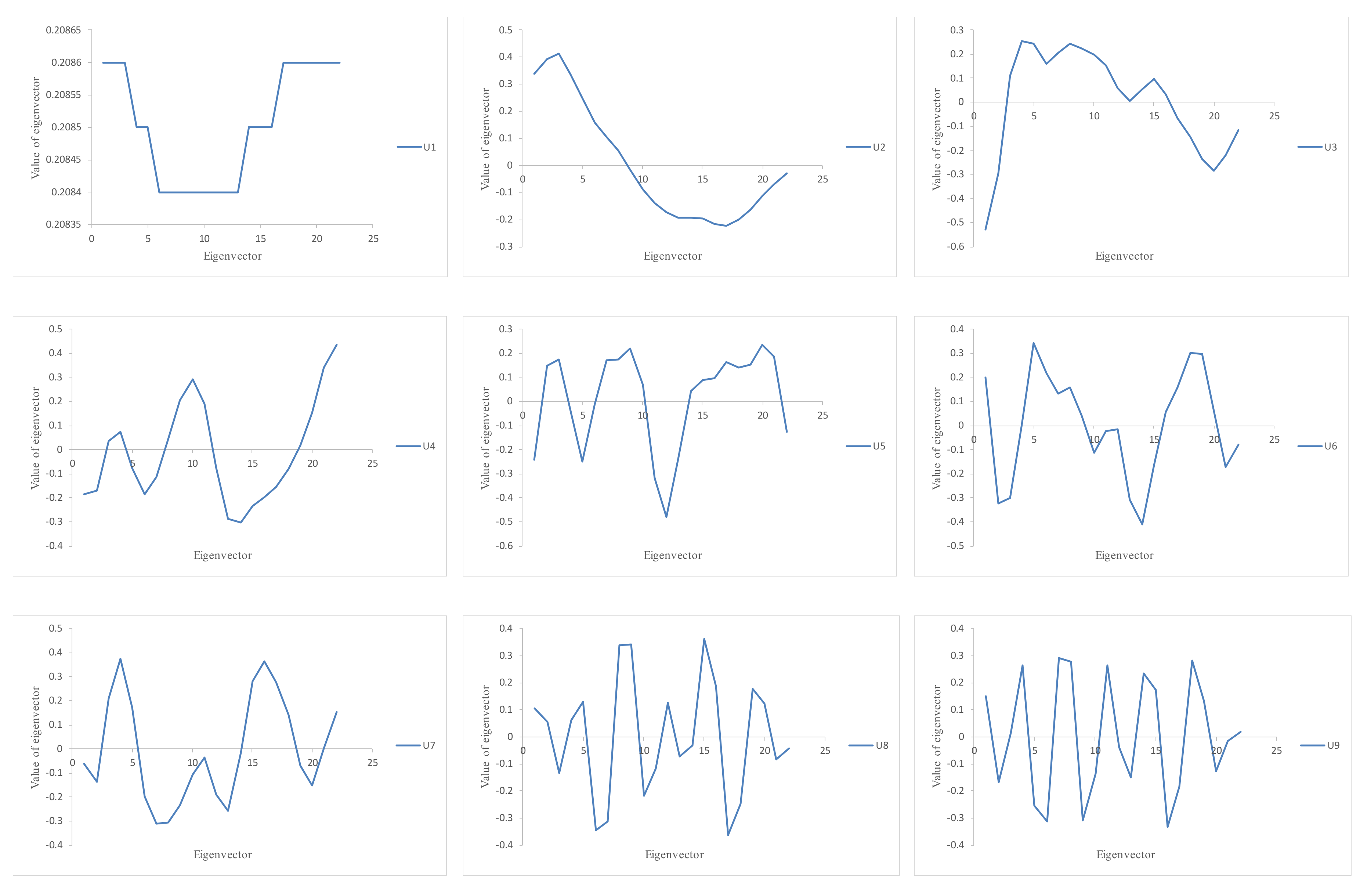
The SVD of matrix
Y is based on the spectral decomposition of the lag-covariance matrix
. Denote
as the eigenvalues of
, arranged in decreasing order
, and
the corresponding eigenvectors. The SVD of the trajectory matrix
Y can be represented as
where
d is the rank of
Y.
The second stage of the algorithm, called reconstruction, includes the following two steps: grouping and diagonal averaging or Hankelization.
The grouping step corresponds to the splitting of the set of matrices
into several disjointed subsets and the summing of the matrices within each subset. The procedure of choosing the subsets
is called grouping. As a simple case, where we have only signal and noise components (
k = 2), we use two subsets,
and
, and associate the subset
with the signal component and the subset
with noise. Selecting the appropriate number of eigenvalues (
r) to be included into the reconstruction is very important. If we take an
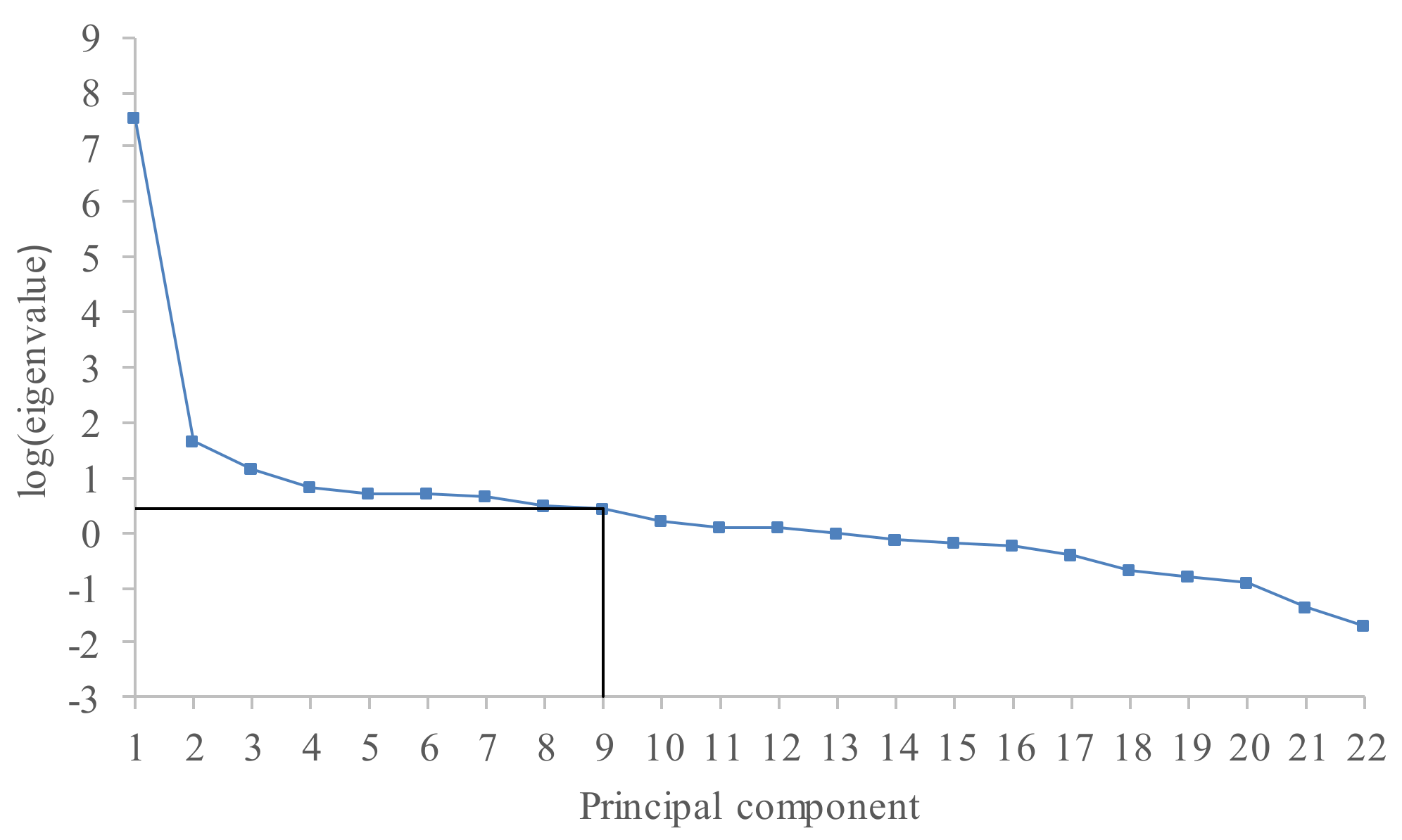
r smaller than it should really be, some parts of the signal will be lost and the accuracy of the reconstructed series will be lower. On the other hand, if the value of
r is too large, then a lot of noise will be included into the reconstructed series. After performing a singular value decomposition of the trajectory matrix, singular values ordered in a decreasing manner are obtained. The plot of the logarithms of the obtained singular values gives very useful information regarding breaks in the eigenvalue spectra. The component where a significant drop in values occurs can be interpreted as the start of the noise floor [
28].
Diagonal averaging or Hankelization represents the last step in SSA, where each reconstructed trajectory matrix (see Equation (16)) is transformed into a new one-dimensional time series of length
N. This corresponds to the averaging of the matrix elements over the anti-diagonals
i +
j=
k + 1; the selection
k = 1 gives
, for
k = 2,
,
and so on. For example, the reconstructed trajectory matrix
is transformed into a new one-dimensional time series
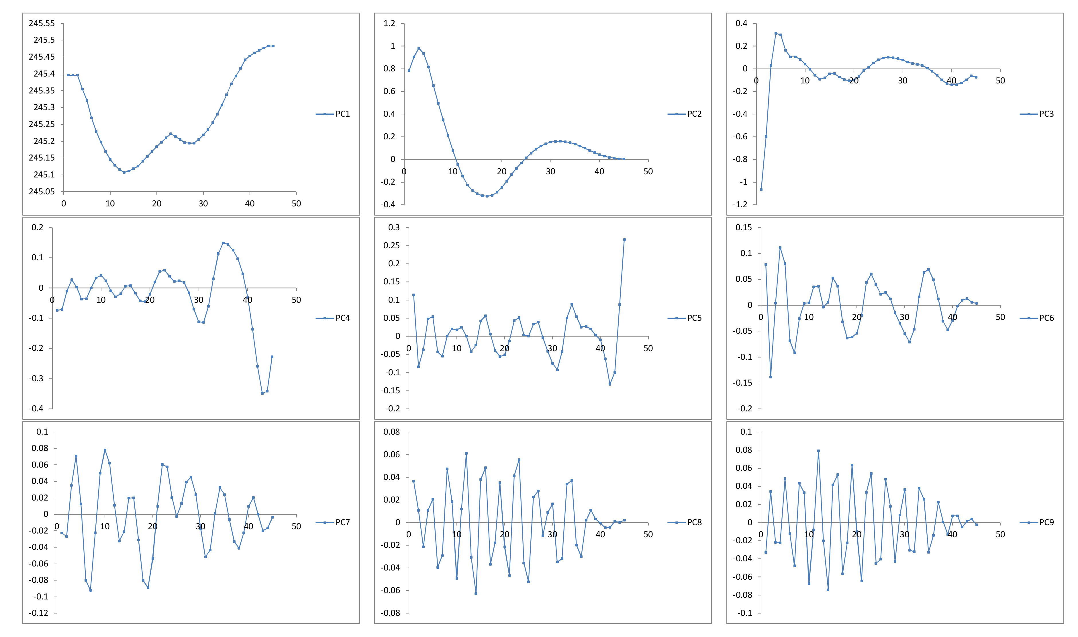
. Finally, the original time series
CN is decomposed into a sum of
r vectors or principal components:
The reconstructed (extracted) series will be used to forecast new data points.
The third stage of the algorithm concerns the future states of the groundwater level and is based on the linear recurrent formulae. Let denote the vector of the first L-1 coordinates of the eigenvectors and indicate the last coordinate of the eigenvectors . Define the verticality coefficient as
If
, then the
h-step ahead SSA forecasting exists. Obviously, the value of
r must be carefully selected to satisfy the previous inequality, as well as to separate the signal from the noise components. The main concept behind the definition of the value of
r is related to the dependence between the different reconstructed (principal) components [
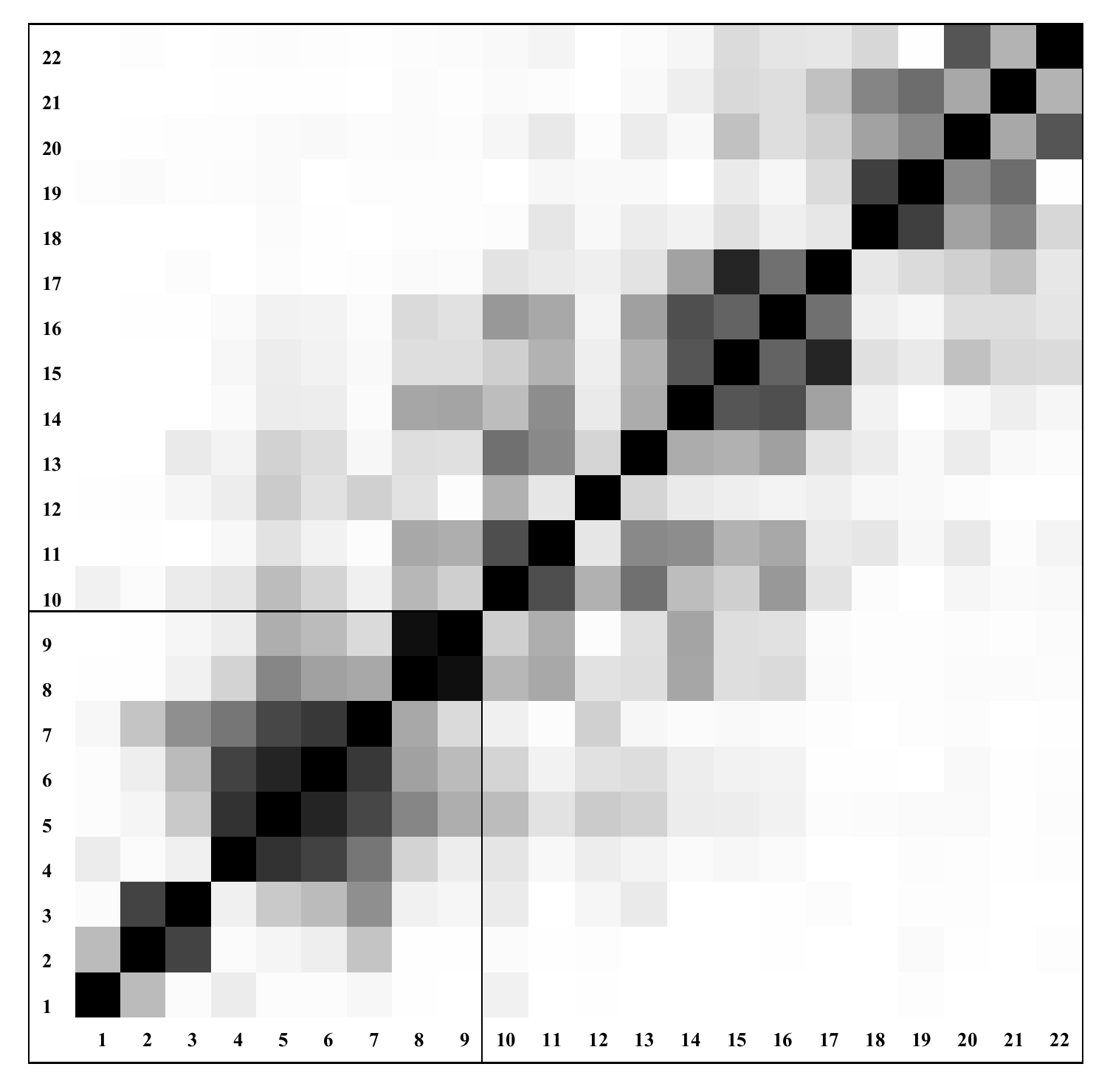
28]. The weighted correlation represents the level of dependence between the two series
and
:
where
—absolute value of the weighted Frobenius inner product,
—the weighted norm
—vector of weights.
If the two reconstructed components have zero
w-correlation, it means that these two components are well separated. Large values of
w-correlations between the reconstructed components indicate that the components should possibly be gathered into one group and correspond to the same component in SSA decomposition [
28]. The obtained correlations can be effectively represented by the
grey-scaled correlation matrix.
The linear vector of coefficients
is calculated as follows:
The
h-step ahead SSA forecasting is achieved by the following equation:
where
The accuracy of the proposed model is estimated by the mean absolute percentage error (
MAPE) and the coefficient of determination (
R2):
where
s(
t) is the actual value,
is the forecasted value of the cluster center and
is the average of the observed set.
R2 is a positive number which demonstrates how well the model fits the data. It can take values between zero and one, where zero indicates that there is a poor correlation between the model output and the actual data. Note, there is a difference between the actual
and the forecasted value
of the cluster center. The sequence of the forecasted cluster centers is now transformed into a sequence of the actual centers by Equation (11);
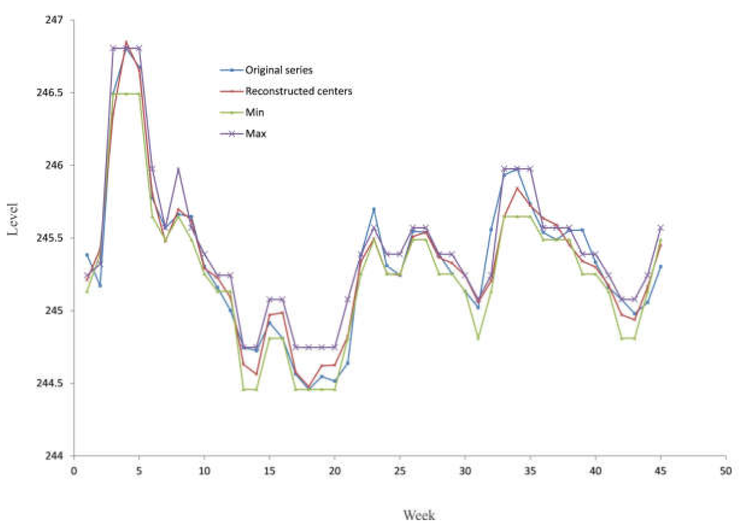
.
According to the concept of the C-mean clustering algorithm, each fuzzy state can be defined as a triplet; , where is equal to the element of the cluster with the minimum value, is equal to the element with the maximum value and has already been explained. Finally, the developed model produces the interval time series .


