Positive Surge Propagation in Sloping Channels


Abstract
:1. Introduction
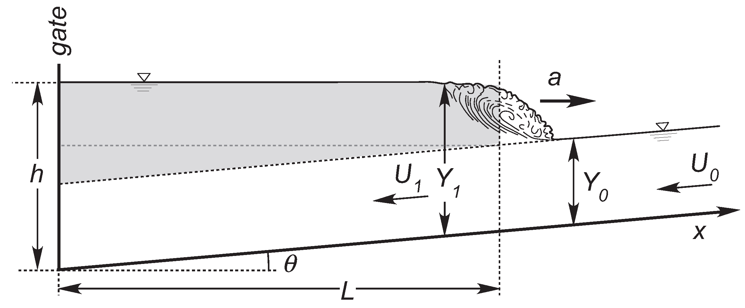
2. The Model
An Approximate Analytical Solution
3. Numerical and Laboratory Experiments
3.1. Laboratory Setup and Experimental Procedures
3.2. The Numerical Model
4. Discussion
4.1. Comparison between the 0D Model Prediction and the Laboratory Experiments
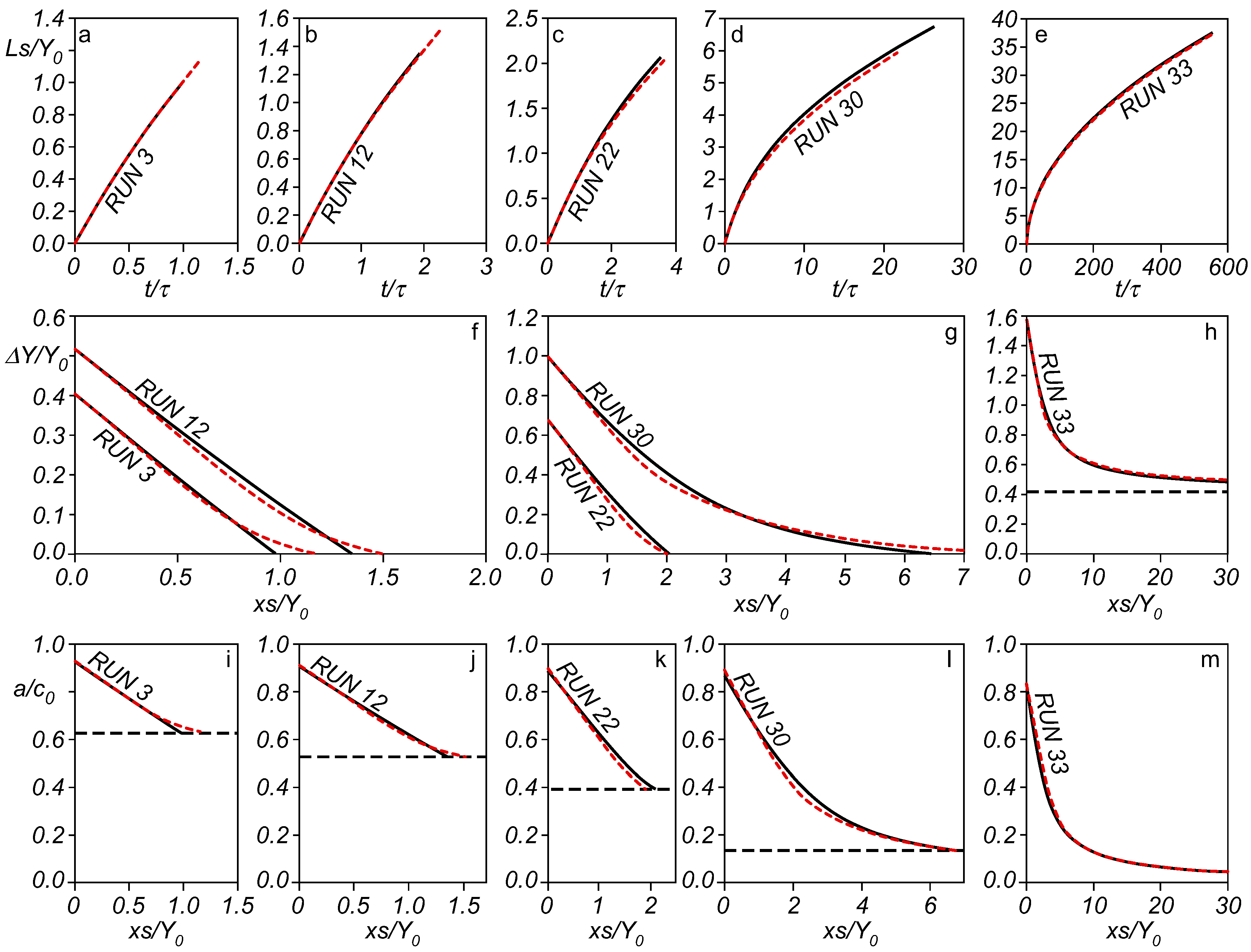
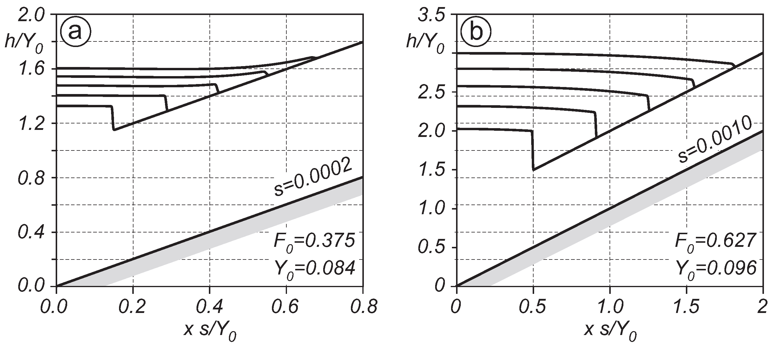
4.2. Comparison between Model Prediction and the Numerical Experiments
5. Conclusions
Acknowledgments
Author Contributions
Conflicts of Interest
Appendix A. Numerical Solution of Model Equations
References
- Castro-Orgaz, O.; Chanson, H. Ritter’s dry-bed dam-break flows: Positive and negative wave dynamics. Environ. Fluid Mech. 2017, 17, 665–694. [Google Scholar] [CrossRef]
- Triki, A. Resonance of free-surface waves provoked by floodgate maneuvers. J. Hydrol. Eng. 2014, 19, 1124–1130. [Google Scholar] [CrossRef]
- Triki, A. Further investigation on the resonance of free-surface waves provoked by floodgate maneuvers: Negative surge waves. Ocean Eng. 2017, 133, 133–141. [Google Scholar] [CrossRef]
- Valiani, A.; Caleffi, V.; Zanni, A. Case Study: Malpasset Dam-Break Simulation using a Two-Dimensional Finite Volume Method. J. Hydraul. Eng. ASCE 2002, 128, 460–472. [Google Scholar] [CrossRef]
- Viero, D.P.; D’Alpaos, A.; Carniello, L.; Defina, A. Mathematical modeling of flooding due to river bank failure. Adv. Water Resour. 2013, 59, 82–94. [Google Scholar] [CrossRef]
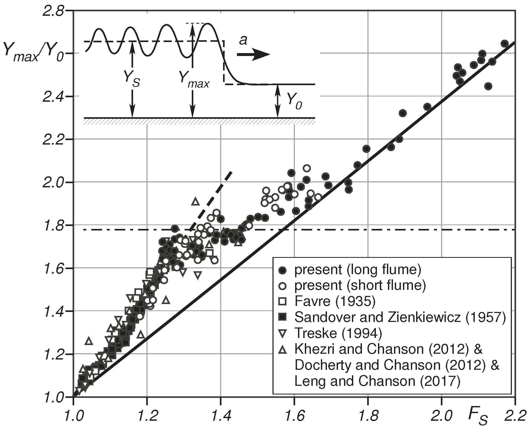
- Favre, H. Etude Théoretique et Expérimentale des Ondes de Translation Dans les Canaux Découverts; Dunod: Paris, France, 1935. [Google Scholar]
- Benjamin, T.B.; Lighthill, M.J. On cnoidal waves and bores. Proc. R. Soc. Lond. Ser. A 1954, 224, 448–460. [Google Scholar] [CrossRef]
- Peregrin, D.H. Calculations of the development of an undular bore. J. Fluid Mech. 1966, 25, 321–330. [Google Scholar] [CrossRef]
- Chanson, H. Undular Tidal Bores: Basic Theory and Free-surface Characteristics. J. Hydraul. Eng. ASCE 2010, 136, 940–944. [Google Scholar] [CrossRef]
- Chanson, H. Turbulent shear stresses in hydraulic jumps, bores and decelerating surges. Earth Surf. Process. Landf. 2011, 36, 180–189. [Google Scholar] [CrossRef]
- Khezri, N.; Chanson, H. Undular and Breaking Tidal Bores on Fixed and Movable Gravel Beds. J. Hydraul. Res. 2012, 50, 353–363. [Google Scholar] [CrossRef]
- Docherty, J.; Chanson, H. Physical modeling of unsteady turbulence in breaking tidal bores. J. Hydraul. Eng. ASCE 2012, 138, 412–419. [Google Scholar] [CrossRef]
- Leng, X.; Chanson, H. Coupling between free-surface fluctuations, velocity fluctuations and turbulent Reynolds stresses during the upstream propagation of positive surges, bores and compression waves. Environ. Fluid Mech. 2016, 16, 695–719. [Google Scholar] [CrossRef]
- Ben Meftah, M.; Mossa, M.; Pollio, A. Considerations on shock wave/boundary layer interaction in undular hydraulic jumps in horizontal channels with a very high aspect ratio. Eur. J. Mech. B Fluids 2010, 29, 415–429. [Google Scholar] [CrossRef]
- Castro-Orgaz, O.; Chanson, H. Minimum Specific Energy and Transcritical Flow in Unsteady Open-Channel Flow. J. Irrig. Drain. Eng. ASCE 2016, 142, 351–363. [Google Scholar] [CrossRef]
- Leng, X.; Chanson, H. Upstream Propagation of Surges and Bores: Free-Surface Observations. Coast. Eng. J. 2017, 59, 1750003. [Google Scholar] [CrossRef]
- Stoesser, T.; McSherry, R.; Fraga, B. Secondary Currents and Turbulence over a Non-Uniformly Roughened Open-Channel Bed. Water 2015, 7, 4896–4913. [Google Scholar] [CrossRef]
- Viero, D.P.; Defina, A. Extended theory of hydraulic hysteresis in open channel flow. J. Hydraul. Eng. ASCE 2017, 143, 06017014. [Google Scholar]
- Viero, D.P.; Defina, A. Multiple states in the flow through a sluice gate. J. Hydraul. Res. 2017. under review. [Google Scholar]
- Viero, D.P.; Pradella, I.; Defina, A. Free surface waves induced by vortex shedding in cylinder arrays. J. Hydraul. Res. 2017, 55, 16–26. [Google Scholar] [CrossRef]
- Henderson, F.M. Open-Channel Flow; McMillan Publishing Co.: New York, NY, USA, 1966. [Google Scholar]
- Defina, A.; Susin, F.M.; Viero, D.P. Bed friction effects on the stability of a stationary hydraulic jump in a rectangular upward sloping channel. Phys. Fluids 2008, 20, 036601. [Google Scholar] [CrossRef]
- Visconti, F.; Stefanon, L.; Camporeale, C.; Susin, F.; Ridolfi, L.; Lanzoni, S. Bed evolution measurement with flowing water in morphodynamics experiments. Earth Surf. Process. Landf. 2012, 37, 818–827. [Google Scholar] [CrossRef]
- Defina, A.; Susin, F.M.; Viero, D.P. Numerical study of the Guderley and Vasilev reflections in steady two-dimensional shallow water flow. Phys. Fluids 2008, 20, 097102. [Google Scholar] [CrossRef]
- Defina, A.; Viero, D.P.; Susin, F.M. Numerical simulation of the Vasilev reflection. Shock Waves 2008, 18, 235–242. [Google Scholar] [CrossRef]
- Viero, D.P.; Susin, F.; Defina, A. A note on weak shock wave reflection. Shock Waves 2013, 23, 505–511. [Google Scholar] [CrossRef]
- Begnudelli, L.; Sanders, B.F. Unstructured Grid Finite-Volume Algorithm for Shallow-Water Flow and Scalar Transport with Wetting and Drying. J. Hydraul. Eng. ASCE 2006, 132, 371–384. [Google Scholar] [CrossRef]
- Defina, A.; Viero, D.P. Open channel flow through a linear contraction. Phys. Fluids 2010, 22, 036602. [Google Scholar] [CrossRef]
- Begnudelli, L.; Sanders, B.F.; Bradford, S.F. Adaptive Godunov-Based Model for Flood Simulation. J. Hydraul. Eng. ASCE 2008, 134, 714–725. [Google Scholar] [CrossRef]
- Sanders, B.F. Integration of a shallow water model with a local time step. J. Hydraul. Res. 2008, 46, 466–475. [Google Scholar] [CrossRef]
- Koch, C.; Chanson, H. Turbulence measurements in positive surges and bores. J. Hydraul. Res. 2009, 47, 29–40. [Google Scholar] [CrossRef]
- Prüser, H.H.; Zielke, W. Undular bores (Favre Waves) in Open Channels Theory and Numerical Simulation. J. Hydraul. Res. 1994, 32, 337–354. [Google Scholar] [CrossRef]
- Castro-Orgaz, O.; Hager, W.H.; Dey, S. Depth-averaged model for undular hydraulic jump. J. Hydraul. Res. 2015, 53, 351–363. [Google Scholar] [CrossRef]
- Sandover, J.A.; Ziekiewicz, P. Experiments on Surge Waves. Water Power 1957, 9, 418–424. [Google Scholar]
- Treske, A. Undular bores (Favre-waves) in open channels—Experimental studies. J. Hydraul. Res. 1994, 32, 355–370. [Google Scholar] [CrossRef]


| Run | s | ||||
|---|---|---|---|---|---|
| (-) | (m/s) | (m) | (-) | (-) | |
| 1–7 | 0.0002 | 0.23–0.41 | 0.045–0.165 | 0.31–0.35 | 1.19–1.28 |
| 8–14 | 0.0005 | 0.27–0.51 | 0.038–0.131 | 0.45–0.46 | 1.31–1.36 |
| 15–23 | 0.0010 | 0.24–0.60 | 0.022–0.112 | 0.53–0.61 | 1.28–1.49 |
| 24–32 | 0.0022 | 0.31–0.81 | 0.015–0.085 | 0.70–0.86 | 1.46–1.69 |
| 33–41 | 0.0052 | 0.43–1.13 | 0.011–0.062 | 1.08–1.41 | 1.75–2.17 |
| 42–49 | 0.0005 | 0.18–0.43 | 0.047–0.154 | 0.26–0.35 | 1.18–1.25 |
| 50–57 | 0.00075 | 0.23–0.47 | 0.036–0.142 | 0.38–0.41 | 1.25–1.34 |
| 58–65 | 0.0010 | 0.25–0.53 | 0.034–0.126 | 0.43–0.48 | 1.28–1.38 |
| 66–73 | 0.0025 | 0.32–0.72 | 0.026–0.093 | 0.64–0.81 | 1.39–1.67 |
| s | ||
|---|---|---|
| (-) | (ms) | (-) |
| 0.0002 | 30–90 | 0.31–0.35 |
| 0.0005 | 25–95 | 0.45–0.46 |
| 0.0010 | 15–90 | 0.53–0.61 |
| 0.0020 | 20–90 | 0.53–0.61 |
| 0.0050 | 80–90 | 1.30–1.75 |
© 2017 by the authors. Licensee MDPI, Basel, Switzerland. This article is an open access article distributed under the terms and conditions of the Creative Commons Attribution (CC BY) license (http://creativecommons.org/licenses/by/4.0/).
Share and Cite
Viero, D.P.; Peruzzo, P.; Defina, A. Positive Surge Propagation in Sloping Channels. Water 2017, 9, 518. https://doi.org/10.3390/w9070518
Viero DP, Peruzzo P, Defina A. Positive Surge Propagation in Sloping Channels. Water. 2017; 9(7):518. https://doi.org/10.3390/w9070518
Chicago/Turabian StyleViero, Daniele Pietro, Paolo Peruzzo, and Andrea Defina. 2017. "Positive Surge Propagation in Sloping Channels" Water 9, no. 7: 518. https://doi.org/10.3390/w9070518
APA StyleViero, D. P., Peruzzo, P., & Defina, A. (2017). Positive Surge Propagation in Sloping Channels. Water, 9(7), 518. https://doi.org/10.3390/w9070518