Article

Assessing the Efficacy of the SWAT Auto-Irrigation Function to Simulate Irrigation, Evapotranspiration, and Crop Response to Management Strategies of the Texas High Plains

1
Department of Ecosystem Science and Management, Texas A&M University, 2138 TAMU, College Station, TX 77845, USA
2
USDA-ARS Conservation and Production Research Laboratory, 2300 Experiment Station Rd., P.O. Drawer 10, Bushland, TX 79012, USA
3
Texas A&M AgriLife Research, Texas A&M AgriLife Research and Extension Center, 6500 Amarillo Blvd W Amarillo, TX 79106, USA
*
Author to whom correspondence should be addressed.
Water 2017, 9(7), 509; https://doi.org/10.3390/w9070509
Submission received: 26 May 2017 / Revised: 29 June 2017 / Accepted: 7 July 2017 / Published: 12 July 2017

Abstract

:
In the semi-arid Texas High Plains, the underlying Ogallala Aquifer is experiencing continuing decline due to long-term pumping for irrigation with limited recharge. Accurate simulation of irrigation and other associated water balance components are critical for meaningful evaluation of the effects of irrigation management strategies. Modelers often employ auto-irrigation functions within models such as the Soil and Water Assessment Tool (SWAT). However, some studies have raised concerns as to whether the function is able to adequately simulate representative irrigation practices. In this study, observations of climate, irrigation, evapotranspiration (ET), leaf area index (LAI), and crop yield derived from an irrigated lysimeter field at the USDA-ARS Conservation and Production Research Laboratory at Bushland, Texas were used to evaluate the efficacy of the SWAT auto-irrigation functions. Results indicated good agreement between simulated and observed daily ET during both model calibration (2001–2005) and validation (2006–2010) periods for the baseline scenario (Nash-Sutcliffe efficiency; NSE ≥ 0.80). The auto-irrigation scenarios resulted in reasonable ET simulations under all the thresholds of soil water deficit (SWD) triggers as indicated by NSE values > 0.5. However, the auto-irrigation function did not adequately represent field practices, due to the continuation of irrigation after crop maturity and excessive irrigation when SWD triggers were less than the static irrigation amount.

1. Introduction

Hydrologic models such as the Soil and Water Assessment Tool (SWAT) [1], Agricultural Policy/Environmental eXtender (APEX) [2], and European Hydrological System Model MIKE SHE [3], are widely used for assessing the impacts of best management practices at various spatial scales. Proper calibration and validation of models using observed data are required for meaningful evaluation of outputs and subsequent use in decision making. In most studies, hydrologic models were calibrated for streamflow using measured data at the watershed outlet [4]. A limited number of studies have used measured evapotranspiration (ET) for calibrating hydrologic models [5,6,7]. According to an assessment of 257 process-based, watershed modeling papers published between 1992 and 2010, Wellen et al. [4] found that in 96% of studies, models were calibrated against measured streamflow, and in the remaining 4% of studies, models were calibrated using measured surface runoff. They found that none of the studies evaluated the ability of the model to simulate any other hydrologic parameters. Researchers have cautioned that model calibrations based on a single measured hydrologic parameter could lead to incorrect conclusions, as errors in the simulation of one hydrologic parameter can be compensated by errors in the simulation of another hydrologic parameter with the opposite sign [8,9]. Modelers have therefore emphasized the need for using other observed hydrologic data in addition to streamflow for calibrating hydrologic models. Among hydrologic parameters, ET is commonly the most significant portion, particularly in semi-arid regions.
Recently, measured long-term lysimeter ET data from the USDA-ARS Conservation and Production Research Laboratory (CPRL) at Bushland, Texas were used for the calibration and validation of the SWAT model for row crops under irrigated and dryland management [5,6]. Detailed weather, plant growth, water balance, agronomy, and management records from the weighing lysimeter fields were also used. The availability of such detailed field-scale data for model calibration is essential for improving model performance. Additionally, long-term observed irrigation data present an opportunity for quantitative analysis of the performance of the auto-irrigation function in hydrologic models. In this study, the open-source SWAT model was used, and the source code was obtained from [10].
Auto-irrigation function in SWAT is based upon one of two water stress trigger (WSTRS_ID) approaches; (1) plant water demand, or (2) soil water content. The plant water demand trigger applies water whenever a user-defined reduction in plant growth occurs (AUTO_WSTRS) due to water stress. However, actual field irrigation is commonly scheduled in response to changes in soil water content in the plant rooting zone. This management approach is most closely represented in SWAT by the soil water content approach, triggered by a user-defined soil water deficit (SWD) threshold (AUTO_WSTRS), calculated as the difference between field capacity and soil water content in mm of water. Lower values of SWD thresholds generally result in more frequent irrigations, as the time required for soil water content to reach the SWD threshold is relatively short. As for larger values of SWD thresholds, the time elapsed between irrigations is increased, as more time is associated with the additional allowed depletion of soil profile water before reaching the SWD threshold. For the same reasons, the first irrigation of the season will generally occur earlier for smaller SWD values, as opposed to later with larger SWD values. Once triggered, irrigation is applied at a user-defined amount (IRR_MX) [11]. If no value is provided, SWAT assigns a default irrigation amount of 25.4 mm (1 inch). This is not reported in the user manual and theoretical documentation but can be identified by the source code. The default irrigation amount and user-defined SWD threshold establish a pseudo field capacity value used to trigger irrigations.
In semi-arid/arid regions, it is not always desirable or even possible to irrigate to field capacity for producers with limited irrigation system capacities. In most cases, producers use a percentage of plant available water (PAW) depletion to trigger irrigations. This managed allowable depletion (MAD) approach allows for more effective use of limited water resources and is dependent upon respective soil and crop characteristics. The difference between this producer–irrigation paradigm and the current auto-irrigation function in SWAT may influence the accurate simulation of irrigation and other water balance parameters. Some studies have qualitatively reported that the auto-irrigation functions in SWAT were unable to appropriately reproduce the hydrologic cycle in the intensively irrigated watersheds [12,13,14,15]. Using SWAT2005, Dechmi et al. [13] commented that the default auto-irrigation functions returned excess irrigation water to the irrigation source, rather than accounting for it in the water balance. Githui et al. [16] also found that monthly patterns of irrigation intervals simulated using the SWAT auto-irrigation function did not match estimated irrigation data of 2009 and 2010 from an irrigated catchment in southeast Australia. Researchers have also recommended different growth stage-specific irrigation techniques to create favorable conditions for crop growth [17]. However, the current auto-irrigation functions in SWAT cannot simulate differential irrigation of crops based on growth stages. To date, no known study has reported the performance of SWAT auto-irrigation functions for simulations of irrigation, ET, and crop responses using quality, long-term field observations.
In this study, data collected from a lysimeter located in an irrigated field at the USDA-ARS CPRL at Bushland, Texas were used for evaluating the SWAT model. Observed data used in this study included continuous measurement of daily ET, seasonal leaf area index (LAI), annual crop yield, climate data, field operations, and detailed irrigation management records from 2000 to 2010. The primary goal of this study was to assess the efficacy of the SWAT auto-irrigation function to simulate irrigation management strategies typical of the Texas High Plains region, while simultaneously simulating reasonable values for crop yield, LAI, and ET. Specifically, the objectives of this study were to: (1) calibrate the SWAT model for ET, LAI, and crop yield using measured values from a weighing lysimeter field; and (2) compare measured ET, irrigation, LAI, and crop yield to simulated values using SWAT auto-irrigation functions under different SWD thresholds triggered by the soil water content method, and quantitatively determine the shortcomings of the auto-irrigation functions.

2. Materials and Methods

2.1. Study Area

The study area is located at the USDA-ARS CPRL near Bushland, Texas (35.2° N, 102.1° W, ~1170 m above mean sea level). The regional climate is classified as semi-arid, with a mean precipitation and temperature (2000–2010) of 488 mm and 14.1 °C, respectively. The major soil is well-drained Pullman silty clay loam (fine, mixed, superactive, thermic Torrertic Paleustoll) [18]. The study area is relatively flat, with a slope of <0.2%. A 4.7 ha irrigated field with a large-weighing lysimeter located in its center was selected as the research site. An adjacent research-grade weather station maintained in accordance with ASCE-EWRI specifications [19] was used for the climate data input. Data collected from the lysimeter field from 2000 to 2010 were processed and used in this study. Crops grown during the study period included cotton (Gossypium hirsutum L.), soybean (Glycine max L.), grain and forage sorghum [Sorghum bicolor (L.) Moench], sunflower (Helianthus annuus L.), and forage corn (Zea mays L.). A linear move sprinkler irrigation system was used to apply water to the crops. The specific crop management practices are listed in Table 1.

2.2. Climate Data Collection and Analysis

Climate data output values (15-min interval) obtained from the research grass reference weather station adjacent to the irrigated lysimeter field were integrated into daily values. These values were used to compute daily weather values for use in the model simulations. Quality assurance and quality control (QA/QC) procedures were used to ensure that measured wind speed, air temperature, precipitation, relative humidity, and solar radiation values were within acceptable tolerances. In addition, all climate data were compared to data collected from a collocated, solar-powered weather station of the Texas High Plains ET Network [20]. Correlations between the two datasets were used to fill any missing climatic data of the research weather station.

2.3. Lysimeter, LAI, and Crop Yield Data Collection and Analysis

The lysimeter contains an undisturbed soil monolith collected on site, weighing ~45 Mg including the container mass. The lysimeter surface dimensions are approximately 3 m × 3 m (9 m2) with a depth of 2.3 m [21]. Voltage outputs from load cells (SM-50, Interface, Inc., Scottsdale, Ariz.) with 22 kg full-range capacity were measured and recorded by data loggers (CR-7X, Campbell Scientific, Logan, Utah) at 0.5 Hz (2 s) frequency. The lysimeter’s accuracy has ranged from 0.05 mm [22,23] to 0.01 mm. Experienced support technicians and scientists were responsible for routine lysimeter maintenance and ensuring representativeness of the surrounding field. Load cell voltage outputs were converted to mass using calibration equations, and 5 min means were used to develop a base dataset for subsequent processing [22]. Lysimeter mass (kg) was converted to a mass-equivalent relative lysimeter storage value (mm of water) by dividing it by the relevant surface area of the lysimeter (~9 m2) and the density of water (taken as 1000 kg m−3). Lysimeter design and management are further described by Marek et al. [5]. Daily ET is calculated using the following soil water balance equation.
ET = P + I + R + F + ΔSW
where P is precipitation (mm), I is irrigation (mm), R is the sum of runon and runoff (taken as zero due to furrow diking to minimize runoff in this study), F is flux into or out of the volume (mm, taken as negative when exiting the control volume), and ΔSW is the change in soil water content (mm). The lysimeter is equipped with a vacuum drainage system, which collects profile drainage into partitioned tanks suspended from the bottom of the lysimeter soil tank such that drainage does not change the lysimeter mass. As such, F was assigned a value of zero. Other mass-changing events were flagged and accounted for according to data processing and data QA/QC procedures provided by Marek et al. [24]. Missing or non-suitable periods of lysimeter ET data resulting from lysimeter maintenance, calibrations, agronomic activities, and power outages were not used. Crop LAI was measured periodically during the growing season throughout the 10-year period. At the end of the growing season, crop yield was also collected.

2.4. SWAT Single HRU Setup and Calibration

The SWAT model is a physically-based, continuous, semi-distributed, watershed-scale model with spatially distributed parameters [1]. Primary model inputs include terrain, land use, soil, weather, and management practices [25]. The SWAT auto-irrigation function using the soil water content method triggered an irrigation when the total soil water in the profile fell below field capacity by more than the user defined SWD threshold. In this study, ArcSWAT 2012 (version 2012.10_0.7) was used. Although SWAT is commonly used for watershed-scale studies, many projects have focused on field-scale modeling. Recently, a single hydrologic response unit (HRU) method was described in detail by Moloney et al. [26] and Cibin et al. [27]. The SWAT model divides a watershed into a number of HRUs and aggregates them into subbasins. An HRU is a basic computational unit in the SWAT model that contains unique land use, soil type, and slope characteristics. An HRU in the SWAT model, therefore, serves as a good representation of field conditions. The SWAT model can be set up using a single HRU, and hence asserts the model useful for field-scale assessment. This emerging single-HRU method is a flexible, time-saving method for field-scale simulations.
The irrigated lysimeter field was set up as one HRU using the single-HRU method. A single HRU management file was created to reflect actual agronomic practices performed on their respective dates of operation, including tillage, planting, fertilization, irrigation, and harvesting. Irrigations on the lysimeter field throughout the study period were scheduled to satisfy full irrigation requirements relative to soil water in the root zone (to a depth of 1.5 m), as determined by soil water neutron probe measurements. The soil water deficit thresholds used to schedule the actual irrigation ranged from approximately 10 mm to 100 mm for various crops at different growth stages. Under the baseline scenario, the actual irrigation practices were input into the single-HRU management file. The soil parameters and values used in this study are shown in Table 2. A SWAT model initially calibrated for ET only using the irrigated lysimeter field by Marek et al. [5] was used and further calibrated for LAI and crop yield. The calibrated hydrologic parameters are listed in Table 3. The SWAT model simulation was structured as an 11-year (2000–2010) simulation. The first year was used for the model warm-up period, and the remaining years were divided into calibration (2001–2005) and validation (2006–2010) periods.
The measured field data (e.g., climate, management practices, and maximum LAI for 2000–2010) were manually inputted into the SWAT model. In addition, important hydrologic parameters and initial state variables were taken from published literature [5]. The crop LAI development-related parameters were manually adjusted to obtain the best fit between simulated LAI and the observed data (Table 4). Finally, crop yield parameters were manually adjusted. This approach involved the year-by-year adjustment of crop growth parameters in the SWAT plant database and provided the most accurate simulation of crop LAI, yield, and ET for subsequent evaluation of the auto-irrigation functions in SWAT.

2.5. Auto-irrigation Scenario Design and Assessment

Eight auto-irrigation scenarios were developed using different soil water deficit thresholds by soil layer. SWD triggers of 10, 20 and 36 mm were used for the first soil layer. SWD triggers of 40, 50, 100 and 158 mm were used for the second, and 337 mm was used for the third soil layer. In this study, the frequencies and amounts of actual irrigations were known. Such detailed information is generally not known for use in modeling studies, which is also the primary reason that the auto-irrigation function is used in many SWAT studies. However, parameterization of the auto-irrigation scenarios in this study assumed no knowledge of the frequencies and amounts of actual irrigation. In this way, the effects of auto-irrigation functions using various SWD threshold triggers on model performance could be quantitatively determined. The results could have implications for previous studies using the SWAT auto-irrigation functions. The SWAT model performance for predicting daily ET and crop yield was evaluated using two statistical measures: percent bias (PBIAS) and Nash-Sutcliffe efficiency (NSE) [29] under the baseline and different auto-irrigation scenarios. The PBIAS statistic is a measure of the tendency of the average to be larger or smaller than the observed values, with an optimal value of zero. Positive and negative values indicate overestimation and underestimation, respectively, expressed as a percentage. The NSE statistic represents the relative magnitude of residual variance compared to the variance of measured data. NSE values range from −∞ to 1.0, with 1.0 being the optimal value.

3. Results and Discussion

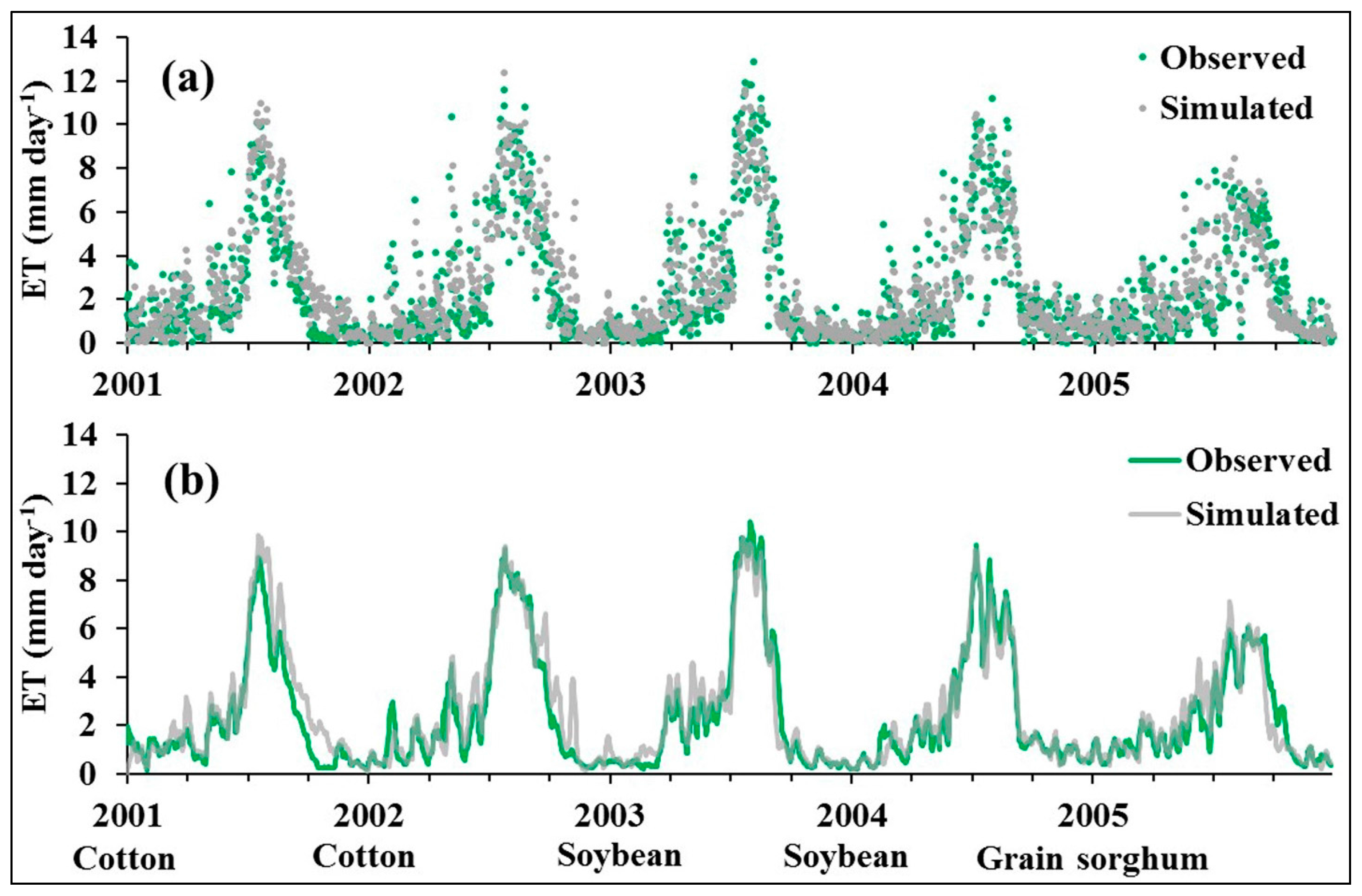
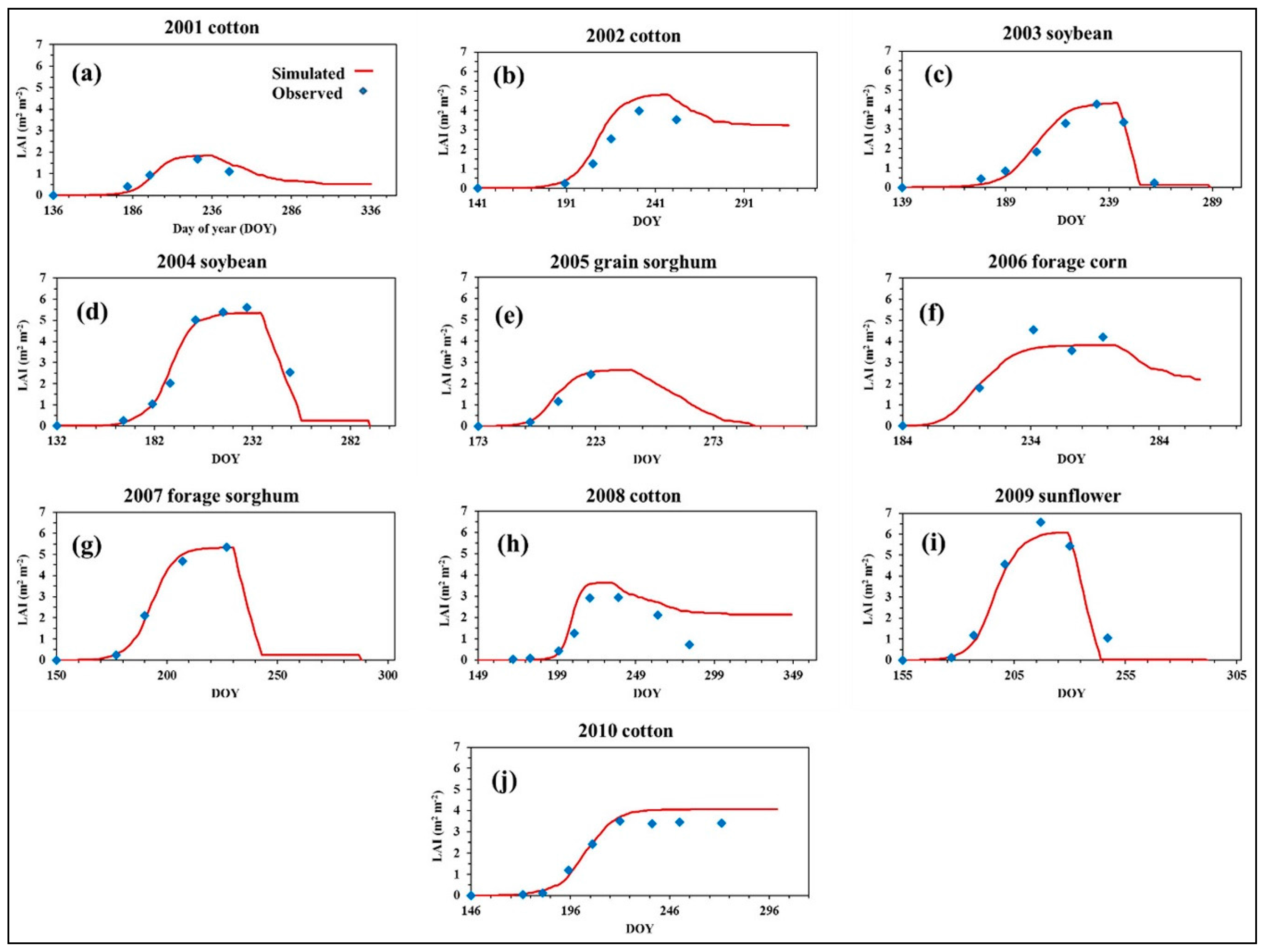
3.1. Evaluation of the SWAT Single-HRU Method for LAI and ET Simulations

The observed maximum LAI values were inputted into the crop database for each crop in each year. Seasonally-measured LAI values were compared to daily-simulated LAI for each year. The graphical comparison indicated that overall, SWAT-simulated LAI matched observed data well (Figure 1). However, SWAT clearly underestimated LAI for forage corn in 2006 (Figure 1f). A large variation in measured LAI for forage corn was also observed in 2006. In that year, the forage corn was damaged by an undetermined plant virus or herbicide, and replanted to a short-season variety in early July. The simulated LAI values of cotton showed an extended tail during the senescence period (Figure 1a,b,h,j), which may result from the lack of application of harvest aids (defoliant) in the SWAT model. Producers commonly apply harvest aids about three weeks prior to expected cotton harvest to facilitate boll opening and maturity, particularly in wetter than normal years. Crop LAI is directly proportional to the transpiration component of ET. A reasonable partition of evaporation and transpiration will benefit the simulations of plant growth and water balance [30].
Following the calibration of LAI, the model performance for ET simulation was evaluated. The NSE and PBIAS values obtained during the model calibration (2001–2005) and validation (2006–2010) periods for the simulation of daily ET from the irrigated lysimeter field were 0.85 and 0.80, and 7.2% and 2.4%, respectively (Table 5). The model performance statistics were deemed “very good” during both calibration and validation periods, according to criteria outlined by Moriasi et al. [31]. Also, NSE model performance was improved as compared to Marek et al. [5] during both the calibration (0.85 vs. 0.67) and validation (0.80 vs. 0.78) periods, due to the further calibration of LAI. The SWAT single-HRU method was, therefore, found to be effective in simulating both LAI and ET. However, simulated ET was slightly higher than the observed ET for cotton in all years during their senescence periods (Figure 2 and Figure 3). This overestimation of ET coincided with the overestimation of LAI during the senescence period of cotton.

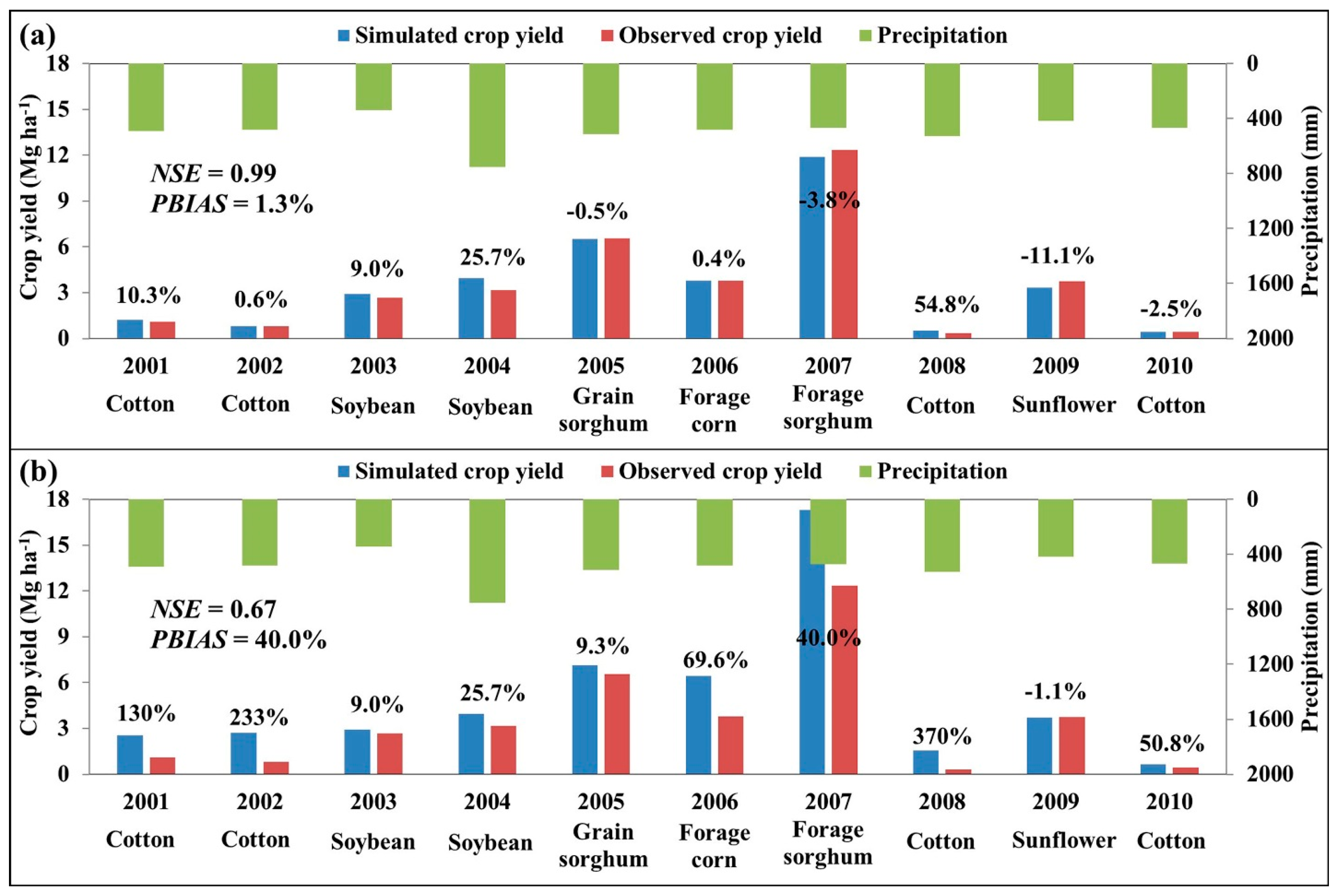
3.2. Comparison of SWAT-Simulated Crop Yields with Field Observations

Some studies have suggested using crop yield as a surrogate for the calibration of ET in SWAT, as crop yield is proportional to the ET component [12,32]. Therefore, after calibrating the model for LAI simulation, the SWAT model was further calibrated for crop yield simulation. The NSE and PBIAS values achieved for the simulation of crop yield during the entire simulation period from 2001 to 2010 were 0.99 and 1.3%, respectively, which represented an excellent agreement between the simulated and observed crop yield (Figure 4a). The detailed field management input is likely the key reason for the accurate crop yield prediction. The evaluation of the SWAT single-HRU method for crop yield simulation enhanced our confidence to use the calibrated model for simulations of ET and crop responses under different auto-irrigation management scenarios.
A large PBIAS resulted for soybean yield in 2004 (25.7%) and cotton yield in 2008 (54.8%). Through a SWAT simulation, Chen et al. [33] also found a large inter-annual variation for irrigated cotton yield simulation in the Southern High Plains of Texas. Another SWAT simulation reported that the simulation accuracy of irrigated cotton yields was much worse than those under dryland conditions (NSE of irrigated and dryland cotton: −0.61 vs. 0.4) in the North Fork River Basin of Southwestern Oklahoma and the Texas Panhandle [34]. Increased precipitation in 2004 and 2008 may have contributed to the large inter-annual variation of soybean in 2004 and cotton in 2008 in this study. Cotton and soybean have perennial crop characteristics, and their indeterminate nature may contribute to their difficulty of simulation. During high rainfall years, cotton and soybean, and particularly cotton, tend to continue growing past their desired growing season. Regarding all other years, the PBIAS was within ±15% (Figure 4a).

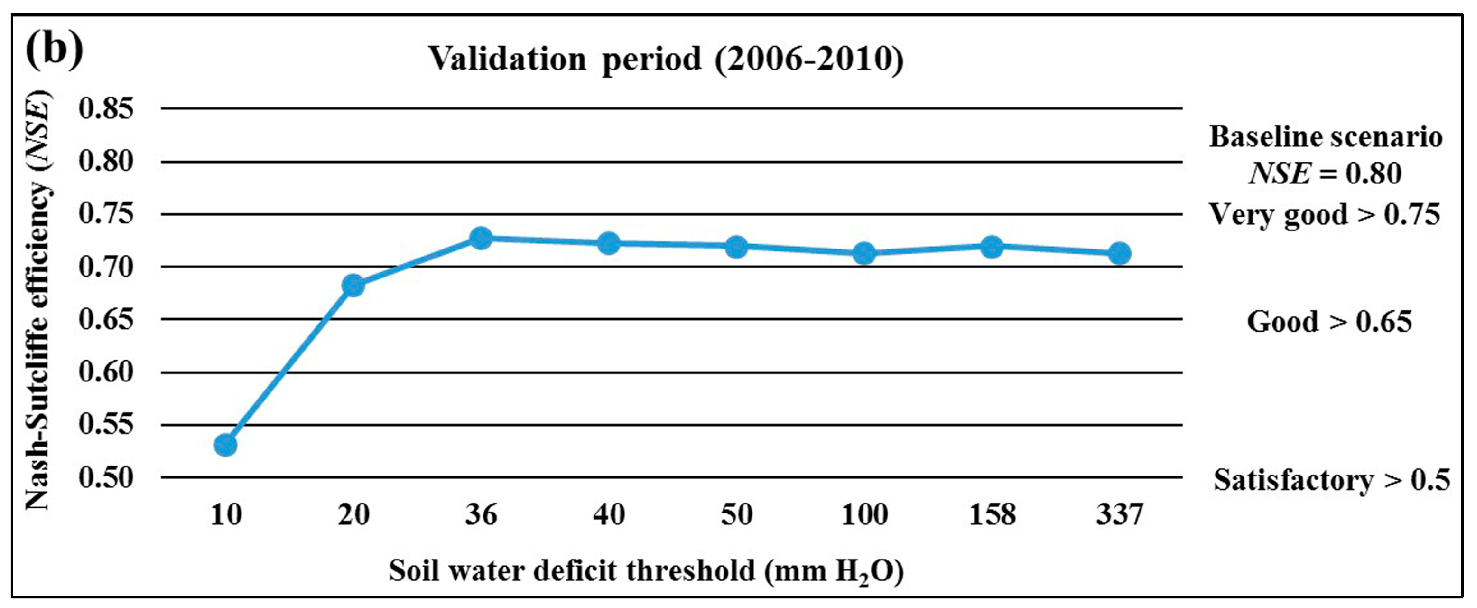
3.3. Simulated ET, Crop Response, and Irrigation Scheduling under SWAT Auto-Irrigation Scenarios

The comparisons of simulated ET during calibration (2001–2005) and validation (2006–2010) periods under different SWD triggers with the measured data indicated that the auto-irrigation functions in SWAT simulated satisfactory values of ET, as compared to measured lysimeter ET (Figure 5). The NSE values were >0.65 during the calibration period under the SWD thresholds from 20 mm to 158 mm, which denoted a good agreement between simulated ET and observed data (Figure 5a). The NSE values of 0.57 and 0.59 resulted from SWD thresholds of 10 mm and 337 mm, respectively. During the validation period, the NSE values were between 0.70 and 0.75 under the SWD thresholds of 36 mm to 337 mm (Figure 5b). Under the SWD thresholds of 10 and 20 mm, the NSE values were 0.53 and 0.68, respectively. The largest NSE values resulted from the SWD threshold of 36 mm (trigger irrigation when the first soil layer lost all plant available water) for both calibration (0.76) and validation (0.73) periods. Although all other measured field data were used in the auto-irrigation scenarios, a noticeable decline in model performance, as compared to the baseline scenario, was still observed in this study (NSE calibration: 0.85 (baseline) vs. 0.76; NSE validation: 0.80 (baseline) vs. 0.73).
Model performance for yield simulations decreased considerably relative to the baseline scenario (Figure 4b). For instance, the NSE and PBIAS values were 0.67 and 40% (baseline NSE and PBIAS: 0.99 and 1.3%) under the auto-irrigation scenario of a SWD threshold of 36 mm, which achieved the best model performance for ET simulation among the auto-irrigation scenarios. Notably, the auto-irrigation scenario simulated substantially higher yields of cotton (>50%), forage corn (70%), and forage sorghum (40%), as compared to the observed data (Figure 4b). As for the LAI values, clear differences were found for cotton in 2002, 2008, and 2010 under the auto-irrigation scenario of a SWD threshold of 36 mm (Figure 6). Cotton is a perennial shrub that is cultivated as an annual cash crop in the U.S. [35]. Vegetative growth continued under well-irrigated conditions. The observed maximum LAI was used as the input for each crop in this study, which was necessary for the reasonable match of the LAI for other crops under the auto-irrigation scenarios.
Interestingly, the SWAT model achieved a good range of model performance in ET simulations under SWD thresholds ranging from 36 mm to 158 mm. This suggests that a large uncertainty in the simulation of hydrologic parameters may exist when using the soil water content method of the auto-irrigation function in the SWAT model. Further analysis of relative amounts of auto-irrigation associated with each SWD trigger was shown in Figure 7. The irrigation amount was set to 25.4 mm (1 inch) in each trigger for all simulations. Therefore, the lower SWD trigger values (10 mm and 20 mm) resulted in frequent irrigations (>300 times vs. 198 times of the baseline scenario) that exceeded field capacity, resulting in the gross overestimation of total irrigation as compared to actual irrigation (Figure 7 and Table 6). Conversely, larger SWD triggers (>40 mm) resulted in corresponding decreases in total simulated irrigation frequencies (<197 times), due to the delay of the initial irrigation, as a greater amount of soil water depletion was allowed before an irrigation event was triggered (Table 6). In general, the actual total seasonal irrigation was approximated to the 36 and 40 mm SWD trigger scenarios. However, total irrigation amounts associated with the majority of SWD thresholds were larger than the actual irrigation amounts for cotton and soybeans (Figure 7). Although the simulated irrigation under different SWD triggers often bracketed actual seasonal irrigation, these simulated values were biased. Use of the soil water content option of the auto-irrigation function resulted in excess irrigation due to the application of irrigation water after crop maturity and in non-growing season. In essence, water is applied strictly based on the SWD trigger and does not terminate following the killing operation. This is a critical flaw in the soil water content method of the SWAT auto-irrigation function. The low NSE values for the 10 mm SWD trigger, during both calibration and validation periods, were caused by excessive irrigation due to the SWD trigger being less than each irrigation amount of 25.4 mm. However, the low NSE value for the 337 mm SWD trigger in the calibration period was likely due to the minimal irrigation applied to the 2004 soybean and 2005 grain sorghum, with both years receiving relatively high amounts of precipitation. Compared to the baseline scenario, the 36 mm and 40 mm SWD triggers showed the most reasonable number of irrigation frequencies (Table 6). However, the differences in irrigation frequency for 2001 and 2010 cotton and 2003 soybean were visible.

4. Conclusions

The accurate simulation of water balance processes and their subsequent impacts on plant growth depend on quality environmental and management inputs. Detailed irrigation management information is crucial for a quantitative evaluation of the change in hydrologic components and crop response under various auto-irrigation scenarios. Several studies have alluded to potential deficiencies of the SWAT auto-irrigation functions to simulate realistic irrigation conditions. Results from this study offered a quantitative analysis of shortcomings of the auto-irrigation functions using long-term observed data. Although the auto-irrigation functions achieved overall satisfactory agreement for ET simulation, a noticeable decrease in NSE (>0.06) was observed, as compared to the baseline scenario. Considerable differences in irrigation amounts and frequencies, as well as crop yields, resulted from a range of SWD triggers, demonstrating that the auto-irrigation functions did not adequately represent field practices. Two major reasons for these results are the continuation of auto irrigation after crop maturity, and excessive irrigation when SWD triggers were less than the static irrigation amount. It is also worth mentioning that the current irrigation trigger factor of soil water content method is not reported as a percentage in the plant water demand option, but rather in terms of mm of soil water deficit, which can easily be overlooked. Findings in this study provide useful information about the potential deficiencies of the SWAT auto-irrigation function for users, modelers, and developers. This study also emphasizes the need for the SWAT auto-irrigation functions to better simulate the water balance and crop growth in an irrigated region. We suggest development of a more sensitive and intuitive auto-irrigation algorithm representative of actual irrigation management, which would greatly improve simulations of study area containing significant irrigated acreages. Managed allowed depletion (MAD), a common conceptual framework for irrigation scheduling, uses a percentage of plant available water to trigger irrigation, rather than only soil characteristics related to the soil water deficit trigger threshold, which may be useful for inclusion in SWAT. The development and testing of MAD-based irrigation algorithms will be the focus of a future study.

Acknowledgments

This research was supported in part by the Ogallala Aquifer Program, a consortium between USDA-Agricultural Research Service, Kansas State University, Texas A&M AgriLife Research, Texas A&M AgriLife Extension Service, Texas Tech University, and West Texas A&M University.

Author Contributions

All authors (Yong Chen, Gary W. Marek, Thomas H. Marek, David K. Brauer, and Raghavan Srinivasan) performed the research and contributed to the writing of the paper.

Conflicts of Interest

The authors declare no conflict of interest.

References

  1. Arnold, J.G.; Srinivasan, R.; Muttiah, R.S.; Williams, J.R. Large-area hydrologic modeling and assessment: Part I. Model development. J. Am. Water Resour. Assoc. 1998, 34, 73–89. [Google Scholar] [CrossRef]
  2. Williams, J.R. The EPIC model. In Computer Models of Watershed Hydrology; Singh, V.P., Ed.; Water Resources Publications: Highlands Ranch, CO, USA, 1995; pp. 909–1000. [Google Scholar]
  3. Refsgaard, J.C.; Storm, B. MIKE SHE. In Computer Models of Watershed Hydrology; Singh, V.P., Ed.; Water Resources Publications: Highlands Ranch, CO, USA, 1995; pp. 809–846. [Google Scholar]
  4. Wellen, C.; Kamran-Disfani, A.; Arhonditsis, G.B. Evaluation of the current state of distributed watershed nutrient water quality modeling. Environ. Sci. Technol. 2015, 49, 3278–3290. [Google Scholar] [CrossRef] [PubMed]
  5. Marek, G.W.; Gowda, P.H.; Evett, S.R.; Baumhardt, R.L.; Brauer, D.K.; Howell, T.A.; Marek, T.H.; Srinivasan, R. Calibration and validation of the SWAT model for predicting daily ET over irrigated crops in the Texas High Plains using lysimetric data. Trans. ASABE 2016, 59, 611–622. [Google Scholar] [CrossRef]
  6. Marek, G.W.; Gowda, P.H.; Evett, S.R.; Baumhardt, R.L.; Brauer, D.K.; Howell, T.A.; Marek, T.H.; Srinivasan, R. Estimating evapotranspiration for dryland cropping systems in the semiarid Texas High Plains using SWAT. J. Am. Water Resour. Assoc. 2016, 52, 298–314. [Google Scholar] [CrossRef]
  7. Jung, C.G.; Lee, D.R.; Moon, J.W. Comparison of the Penman-Monteith method and regional calibration of the Hargreaves equation for actual evapotranspiration using SWAT-simulated results in the Seolma-cheon basin, South Korea. Hydrol. Sci. J. 2016, 61, 793–800. [Google Scholar] [CrossRef]
  8. Beven, K. A manifesto for the equifinality thesis. J. Hydrol. 2006, 320, 18–36. [Google Scholar] [CrossRef]
  9. Kirchner, J.W. Getting the right answers for the right reasons: Linking measurements, analyses, and models to advance the science of hydrology. Water Resour. Res. 2006, 42, W03S04. [Google Scholar] [CrossRef]
  10. SWAT|Soil and Water Assessment Tool—Texas A&M University. Available online: http://swat.tamu.edu/ (accessed on 9 July 2017).
  11. Neitsch, S.L.; Arnold, J.G.; Kiniry, J.R.; Williams, J.R. Soil and Water Assessment Tool Theoretical Documentation Version 2009; Texas Water Resources Institute: College Station, TX, USA, 2011. [Google Scholar]
  12. Akhavan, S.; Abedi-Koupai, J.; Mousavi, S.F.; Afyuni, M.; Eslamian, S.S.; Abbaspour, K.C. Application of SWAT model to investigate nitrate leaching in Hamadan-Bahar Watershed, Iran. Agric. Ecosyst. Environ. 2010, 139, 675–688. [Google Scholar] [CrossRef]
  13. Dechmi, F.; Burguete, J.; Skhiri, A. SWAT application in intensive irrigation systems: Model modification, calibration and validation. J. Hydrol. 2012, 470–471, 227–238. [Google Scholar] [CrossRef]
  14. Chen, Y.; Ale, S.; Rajan, N.; Munster, C. Assessing the hydrologic and water quality impacts of biofuel-induced changes in land use and management. Glob. Chang. Biol. Bioenergy 2017. [Google Scholar] [CrossRef]
  15. Marek, G.W.; Gowda, P.H.; Marek, T.H.; Porter, D.O.; Baumhardt, R.L.; Brauer, D.K. Modeling long-term water use of irrigated cropping rotations in the Texas High Plains using SWAT. Irrig. Sci. 2017, 35, 111–123. [Google Scholar] [CrossRef]
  16. Githui, F.; Thayalakumaran, T.; Selle, B. Estimating irrigation inputs for distributed hydrological modelling: A case study from an irrigated catchment in southeast Australia. Hydrol. Process. 2016, 30, 1824–1835. [Google Scholar] [CrossRef]
  17. Xie, X.; Cui, Y. Development and test of SWAT for modeling hydrological processes in irrigation districts with paddy rice. J. Hydrol. 2011, 396, 61–71. [Google Scholar] [CrossRef]
  18. Unger, P.W.; Pringle, F.B. Pullman Soils: Distribution Importance, Variability, and Management; Bulletin B-1372; Texas Agricultural Experiment Station: College Station, TX, USA, 1981. [Google Scholar]
  19. American Society of Civil Engineers (ASCE). The ASCE Standardized Reference Evapotranspiration Equation; ASCE Environmental and Water Resources Institute: Reston, VA, USA, 2005. [Google Scholar]
  20. Marek, T.H.; Porter, D.O.; Howell, T.A. The Texas High Plains Evapotranspiration Network: An Irrigation Scheduling Technology Transfer Tool; Technical Report for Contract No. 2004-358-008; Texas Water Development Board: Austin, TX, USA, 2005. [Google Scholar]
  21. Marek, T.H.; Schneider, A.D.; Howell, T.A.; Ebeling, L.L. Design and construction of large weighing monolithic lysimeters. Trans. ASAE 1988, 31, 477–484. [Google Scholar] [CrossRef]
  22. Howell, T.A.; Schneider, A.D.; Dusek, D.A.; Marek, T.H.; Steiner, J.L. Calibration and scale performance of Bushland weighing lysimeters. Trans. ASAE 1995, 38, 1019–1024. [Google Scholar] [CrossRef]
  23. Evett, S.R.; Schwartz, R.C.; Howell, T.A.; Baumhardt, R.L.; Copeland, K.S. Can weighing lysimeter ET represent surrounding field ET well enough to test flux station measurements of daily and sub-daily ET? Adv. Water Resour. 2012, 50, 79–90. [Google Scholar] [CrossRef]
  24. Marek, G.W.; Evett, S.R.; Gowda, P.H.; Howell, T.A.; Copeland, K.S.; Baumhardt, R.L. Post-processing techniques for reducing errors in weighing lysimeter evapotranspiration (ET) datasets. Trans. ASABE 2014, 57, 499–515. [Google Scholar] [CrossRef]
  25. Srinivasan, R.; Zhang, X.; Arnold, J.G. SWAT ungauged: Hydrological budget and crop yield predictions in the upper Mississippi river basin. Trans. ASABE 2010, 53, 1533–1546. [Google Scholar] [CrossRef]
  26. Moloney, C.; Cibin, R.; Chaubey, I. Using a Single HRU SWAT Model to Examine and Improve Representation of Field-Scale Processes. 2015. Available online: http://swat.tamu.edu/conferences/international/2015-purdue/material/ (accessed on 9 July 2017).
  27. Cibin, R.; Chaubey, I.; Helmers, M.; Sudheer, K.P.; White, M.; Arnold, J.G. Improved Physical Representation of Vegetative Filter Strip in SWAT. 2015. Available online: http://swat.tamu.edu/conferences/international/2015-purdue/material/ (accessed on 9 July 2017).
  28. Sinnathamby, S.; Douglas-Mankin, K.R.; Craige, C. Field-scale calibration of crop-yield parameters in the Soil and Water Assessment Tool (SWAT). Agric. Water Manag. 2017, 180, 61–69. [Google Scholar] [CrossRef]
  29. Nash, J.E.; Sutcliffe, J.V. River flow forecasting through conceptual models, Part I-a discussion of principles. J. Hydrol. 1970, 10, 282–290. [Google Scholar] [CrossRef]
  30. Yimam, Y.T.; Ochsner, T.E.; Kakani, V.G. Evapotranspiration partitioning and water use efficiency of Switchgrass and biomass sorghum managed for biofuel. Agric. Water Manag. 2015, 155, 40–47. [Google Scholar] [CrossRef]
  31. Moriasi, D.N.; Arnold, J.G.; Van Liew, M.W.; Binger, R.L.; Harmel, R.D.; Veith, T. Model evaluation guidelines for systematic quantification of accuracy in watershed simulations. Trans. ASABE 2007, 50, 885–900. [Google Scholar] [CrossRef]
  32. Faramarzi, M.; Abbaspour, K.C.; Schulin, R.; Yang, H. Modeling blue and green water resources availability in Iran. Hydrol. Process. 2009, 23, 486–501. [Google Scholar] [CrossRef]
  33. Chen, Y.; Ale, S.; Rajan, N.; Morgan, C.L.S.; Park, J.Y. Hydrological responses of land use change from cotton (Gossypium hirsutum L.) to cellulosic bioenergy crops in the Southern High Plains of Texas, USA. Glob. Chang. Biol. Bioenergy 2016, 8, 981–999. [Google Scholar] [CrossRef]
  34. Mittelstet, A.R.; Storm, D.E.; Stoecker, A.L. Using SWAT and an empirical relationship to simulate crop yields and salinity levels in the North Fork River Basin. Int. J. Agric. Biol. Eng. 2015, 8, 110–124. [Google Scholar] [CrossRef]
  35. Ton, P. Cotton and climate change in west Africa. In The Impact of Climate Change on Drylands; Environment & Policy Series; Springer: Dordrecht, The Netherlands, 2004; Volume 39, pp. 97–115. [Google Scholar]
Figure 1. Simulated vs. measured leaf area index (LAI) values for crops under the irrigated lysimeter field from 2001 to 2010.
Water 09 00509 g001
Figure 2. SWAT simulated daily (a) and seven-day running average (b) Evapotranspiration (ET) versus observed ET of the irrigated lysimeter field during the calibration period (2001–2005).
Water 09 00509 g002
Figure 3. SWAT simulated daily (a) and seven-day running average (b) ET versus observed ET of the irrigated lysimeter field during the validation period (2006–2010).
Water 09 00509 g003
Figure 4. Comparison of observed and simulated crop yield under the baseline scenario (a) and under the auto-irrigation scenario of 36 mm soil water deficit trigger (b).
Water 09 00509 g004
Figure 5. Model performance statistic of NSE for daily measured and simulated ET during (a) calibration (2001–2005) and (b) validation (2006–2010) periods under different soil water deficit thresholds using SWAT auto-irrigation functions.
Water 09 00509 g005aWater 09 00509 g005b
Figure 6. Simulated leaf area index (LAI) under the auto-irrigation scenario of 36 mm soil water deficit trigger compared to measured LAI for crops under the irrigated lysimeter field from 2001 to 2010.
Water 09 00509 g006
Figure 7. Irrigation amounts (mm) of actual management and simulated soil water deficit triggers using the auto-irrigation functions in SWAT. Annual total precipitation values are also shown.
Water 09 00509 g007
Table 1. Crops grown on the irrigated lysimeter field from 2000 to 2010.
YearIrrigated CropPlanting DateFertilizer Application (kg ha−1) *Harvest Date
2000Cotton16 May504.46 December
2001Cotton16 May326.23 December
2002Cotton21 May571.613 November
2003Soybean19 MayNot applied15 October
2004Soybean12 MayNot applied19 October
2005Grain sorghum22 June612.07 November
2006Forage corn3 July68.414 December
2007Forage sorghum30 May510.015 October
2008Cotton21 May408.015 December
2009Sunflower4 June510.019 October
2010Cotton26 MayNot applied28 October
Note: * Ammonium nitrate fertilizer.
Table 2. Soil information from the Soil Survey Geographic Database (SSURGO) used in model setup.
Soil InformationLayer 1Layer 2Layer 3Layer 4
Depth (mm)0–180180–860860–18001800–2300
Bulk density (g cm−3)1.431.381.381.45
Available water capacity (mm H2O per mm soil)0.200.180.190.14
Saturated hydraulic conductivity (mm hr−1)9.722.162.169.72
Clay content (% soil mass)33.942.139.439.1
Silt content (% soil mass)53.848.047.647.1
Sand content (% soil mass)12.39.913.013.8
Table 3. Calibrated values of the selected Soil and Water Assessment Tool (SWAT) hydrologic parameters.
ParameterDescriptionRangeCalibrated Value
ESCOPlant uptake compensation factor0.0–1.01.000
EPCOSoil evaporation compensation factor0.0–1.00.900
FFCBInitial soil water storage0.0–1.00.750
EVPOTPothole evaporation coefficient0.0–1.00.5
POT_VOLXMaximum volume of water stored in the pothole (mm) over the entire HRU0–∞50 mm
EVLAILeaf area index at which no evaporation occurs from the water surface0.0–10.04.0
Table 4. Default and calibrated values of crop parameters in Soil and Water Assessment Tool (SWAT).
No.ParameterDescriptionDefault ValueCalibrated ValueSource
2001 cotton
1BLAIMax leaf area index (m2/m2)42Measured *
2FRGRW2Fraction of the plant growing season corresponding to the 2nd point on the optimal leaf area development curve0.50.6Estimated #
3DLAIFraction of the plant growing season when leaf area begins to decline0.950.7Estimated
2002 cotton
1BLAIMax leaf area index (m2/m2)45Measured
2FRGRW1Fraction of the plant growing season corresponding to the 1st point on the optimal leaf area development curve0.150.2Estimated
3FRGRW2Fraction of the plant growing season corresponding to the 2nd point on the optimal leaf area development curve0.50.6Estimated
4DLAIFraction of the plant growing season when leaf area begins to decline0.950.7Estimated
2003 soybean
1BLAIMax leaf area index (m2/m2)34.5Measured
2FRGRW1Fraction of the plant growing season corresponding to the 1st point on the optimal leaf area development curve0.150.3Estimated
3FRGRW2Fraction of the plant growing season corresponding to the 2nd point on the optimal leaf area development curve0.50.8Estimated
4DLAIFraction of the plant growing season when leaf area begins to decline0.60.92Estimated
2004 soybean
1BLAIMax leaf area index (m2/m2)35.5Measured
2FRGRW1Fraction of the plant growing season corresponding to the 1st point on the optimal leaf area development curve0.150.3Estimated
3FRGRW2Fraction of the plant growing season corresponding to the 2nd point on the optimal leaf area development curve0.50.65Estimated
4DLAIFraction of the plant growing season when leaf area begins to decline0.60.85Estimated
2005 grain sorghum
1BLAIMax leaf area index (m2/m2)32.8Measured
2FRGRW1Fraction of the plant growing season corresponding to the 1st point on the optimal leaf area development curve0.150.2Estimated
2006 forage corn
1BLAIMax leaf area index (m2/m2)45Measured
2007 forage sorghum
1BLAIMax leaf area index (m2/m2)45.5Measured
2BIO_EBiomass/energy ratio [(kg ha−1)/(MJ m−2)]33.545Sinnathamby et al. [28]
3FRGRW1Fraction of the plant growing season corresponding to the 1st point on the optimal leaf area development curve0.150.25Estimated
4FRGRW2Fraction of the plant growing season corresponding to the 2nd point on the optimal leaf area development curve0.50.6Estimated
5DLAIFraction of the plant growing season when leaf area begins to decline0.640.84Estimated
2008 cotton
1BLAIMax leaf area index (m2/m2)43.8Measured
2FRGRW1Fraction of the plant growing season corresponding to the 1st point on the optimal leaf area development curve0.150.3Estimated
3DLAIFraction of the plant growing season when leaf area begins to decline0.950.58Estimated
2009 sunflower
1BLAIMax leaf area index (m2/m2)37Measured
2FRGRW1Fraction of the plant growing season corresponding to the 1st point on the optimal leaf area development curve0.150.2Estimated
3FRGRW2Fraction of the plant growing season corresponding to the 2nd point on the optimal leaf area development curve0.50.7Estimated
4DLAIFraction of the plant growing season when leaf area begins to decline0.620.85Estimated
2010 cotton
1BLAIMax leaf area index (m2/m2)45.8Measured
2DLAIFraction of the plant growing season when leaf area begins to decline0.950.8Estimated
Notes: * Field measured maximum leaf area index; # Estimated value based on the pattern of several measured leaf area index values.
Table 5. Model performance statistics for daily measured and simulated ET during calibration (2001–2005) and validation (2006–2010) periods.
Manual Input All the Field Observations (Baseline Scenario)Daily ET
Statistics2001–20052006–2010
Measured mean (mm)2.402.42
Simulated mean (mm)2.582.48
Nash-Sutcliffe efficiency (NSE)0.850.80
Percent bias (PBIAS)7.2%2.4%
Table 6. Irrigation frequencies (number of times) of actual management and simulated soil water deficit triggers using the auto-irrigation functions in SWAT.
Year and CropActual Frequency10 mm *20 mm36 mm40 mm50 mm100 mm158 mm337 mm
2001 cotton185734262524211810
2002 cotton237038252423191712
2003 soybean31693624242320187
2004 soybean16542717161412101
2005 grain sorghum145722121211855
2006 forage corn27683724232015137
2007 forage sorghum1852201413131085
2008 cotton20683423222014116
2009 sunflower175725161615131017
2010 cotton146633222221191870
Total frequencies19861830620319718415112810
Note: * Soil water deficit threshold (mm H2O).

