Variability of Darcian Flux in the Hyporheic Zone at a Natural Channel Bend

Abstract

Channel bends are one of the most important characteristic features of natural streams. These bends often create the conditions for a hyporheic zone, which has been recognized as a critical component of stream ecosystems. The streambed vertical hydraulic conductivity (K_v), vertical hydraulic gradient (VHG) and Darcian flux (DF) in the hyporheic zone were estimated at 61 locations along a channel bend of the Beiluo River during July 2015 and January 2016. All the streambed attributes showed great spatial variability along the channel bend. Both upward fluxes and downward fluxes occurred during the two test periods, most of studied stream sections were controlled by downwelling, indicating stream water discharge into the subsurface. The average downward flux was higher at the downstream side than at the upstream side of the channel bend, especially in July 2015. The distribution of streambed sediment grain size has a significant influence on the variability of K_v; high percentages of silt and clay sediments generally lead to low K_v values. Higher K_v at the depositional left bank at the upstream site shifted toward the erosional right bank at the downstream site, with K_v values positively correlated with the water depth. This study suggested that the variabilities of K_v and VHG were influenced by the stream geomorphology and that the distribution of K_v was inversely related, to a certain extent, to the distribution of VHG across the channel bend. K_v and VHG were found to have opposite effects on the DF, and the close relationship between K_v and DF indicated that the water fluxes were mainly controlled by K_v.

1. Introduction

The hyporheic zone, the transition region from a stream to the surrounding aquifer, acts as a physical, chemical, and biological filter and has been recognized as a critical component of stream ecosystems [1]. The transfer and transformation of nutrients or pollutants between groundwater and the surface water can be promoted or prevented, and solutes and oxygen can migrate into oxic and anoxic environments through hyporheic water flows, resulting in variations of the redox conditions of the sediments and aquifers and ultimately controlling the growth of microorganisms [2,3]. The dissolved oxygen concentration of upwelling stream waters is lower than other stream waters because the reactive solutes and dissolved oxygen could be carried by downwelling fluxes [4]. Therefore, the hyporheic zone plays an important role in protecting the water quality and quantity of streams and groundwater from various pollutant species [5]. The water exchange between streams and their hyporheic zones, termed hyporheic water exchange, is influenced by variations in the hydraulic gradient over the stream channel boundary stemming from geomorphic features, such as stream meanders, bars, dunes, step-pools, and in-stream structures [6,7,8]; a chalk stream overlain by Palaeogene deposits and superficial drift from the Quaternary [9]; or ambient groundwater discharge [10]. The channel bend is one of the characteristic features of all streams and favors the formation of hyporheic zones [11]. It is now understood that the interfacial flux of the stream water and streambed increases with sinuosity and that the meander apex experiences the largest flux [6]. These fluxes toward or away from sinuous streams and hyporheic zones have implications for biogeochemical and ecological processes along the fluvial corridor from the river to riparian zones [12].

Many measurement methods can be used to determine the velocity or flux of the surface water, aquifer and transition zones, including the Darcy equation, tracer tests, temperature gradient, and seepage meters, but these methods all have certain limitations due to different measurement scales and hydrogeological conditions; therefore, it is important to choose the method most appropriate to the study goal to characterize the interaction between rivers and their hyporheic zones [13]. The specific discharge between stream and streambed can be obtained using the Darcian flux calculations employing the hydraulic conductivity and hydraulic gradient. The variability of streambed hydraulic conductivity depends on sedimentary characteristics, especially the distribution of the sediment grain size, and is related to the erosional and depositional processes induced by varying stream flows and influenced by the stream morphology [14,15]. Another parameter characterizing the sedimentary hydrogeological control of hyporheic water exchange is the porosity of sediments [16]. Generally, hydraulic conductivity increases with particle size, but this relation can be modified by changes in overall porosity [17]. The hydraulic gradient is also one of the important streambed attributes used to provide an estimate of the potential strength of a hydrological exchange and has a significant influence on stream infiltration and storage zone in the aquifer [18,19]. The direction and magnitude of Darcian flux vary greatly in different locations due to changes in these two variables, hydraulic conductivity and gradient, spatially and temporally, induced by dynamic environments in the stream, and have been identified as the two main factors controlling water exchange between streams and the surrounding groundwater systems [20,21]. According to various laboratory experiments, the hyporheic water exchange rate is proportional to the square of the stream water velocity and to the permeability of streambed sediments and inversely proportional to the porosity of the sediments and to the depth of the streambed [16]. However, under field experiments, the relationship of these characteristics is not well established, especially in the channel bend of a natural stream.

The objective of this study is to determine the variability of Darcian flux, streambed hydraulic conductivity, and head gradient at a natural channel bend and further reveal the relationship among these three streambed attributes in the hyporheic zone.

2. Study Site and Methods

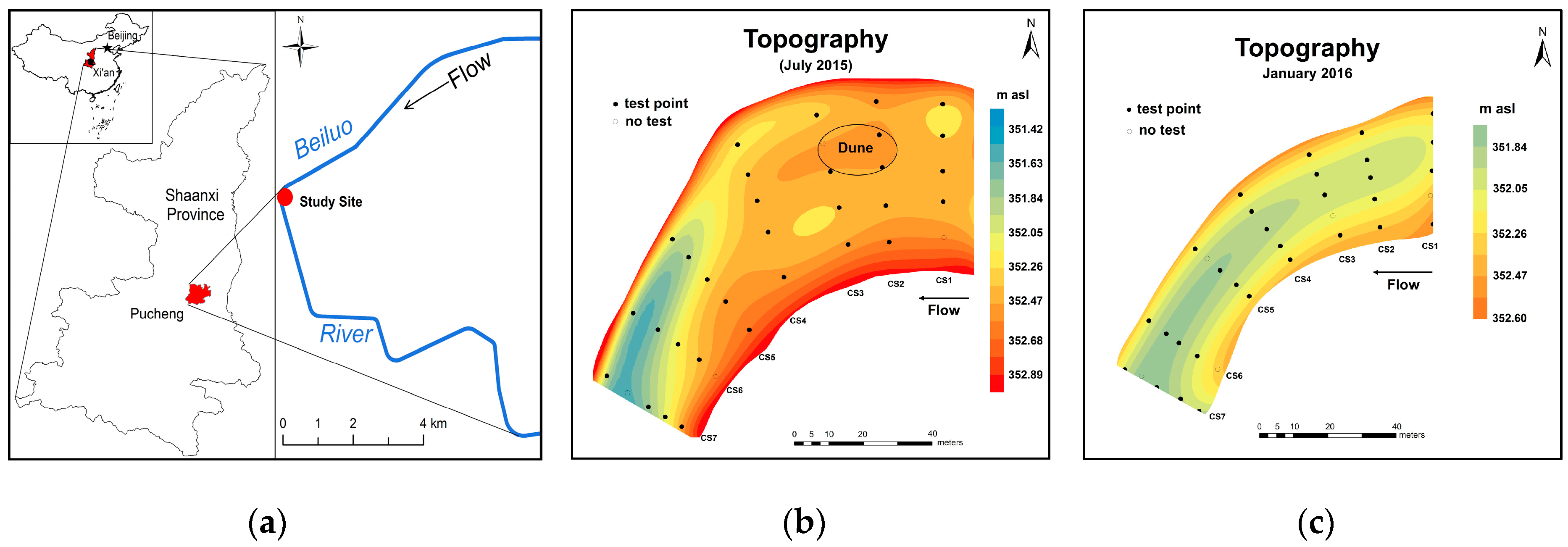
2.1. Study Site

The study was conducted at the Beiluo River in Shaanxi Province in Northwestern China (Figure 1a). The Beiluo River is one of the northern branches of the Weihe River. It flows from northwest to southeast through the Loess Plateau and the Guanzhong Basin and has a total length of 680.3 km, a stream catchment of approximately 2.69 × 10⁴ km², an average stream gradient of 1.98‰ and an annual average stream discharge of 14.99 m³/s. The Beiluo River is located in a semi-arid region with a mean annual precipitation of 400–600 mm and a highly spatially and temporally uneven distribution of precipitation. Approximately 76.2% of annual precipitation occurs during the flood season from May to September [22]. The Beiluo River is a sandy stream, and the streambed sediments are composed of alluvial loess, sandy clay, and Pliocene and Holocene sandy-gravel strata [14]. The Beiluo River basin is an important grain-producing area on the Guanzhong Plain and provides water supplies for agricultural production and human activities. The stream system has diverse landscape types and numerous meanders. Soil erosion is very serious in this basin because a long history of inputs of organic compounds and heavy metals have resulted in changes to the water quality of the Beiluo River.

The study site is located in the downstream region of the Beiluo River in Pucheng County (34°55′ N, 109°48’ E), where the groundwater quality is very poor and has a high fluorine content. The field measurements were conducted in a 120 m long channel bend of the Beiluo River on 7–8 July 2015 and 10–11 January 2016. The right and left sides of the river are characterized by loess terrace and alluvial plain, respectively. The average channel width, water depth and water velocity were higher in July 2015 than in January 2016 and the sinuosity of the channel bend also differed between these two test periods (

Table 1. Flow conditions at the channel bend of the Beiluo River during July 2015 and January 2016.

Flow Condition	July 2015	January 2016
Number of measurements	31	30
Average channel width (m)	29	25
Average water depth (cm)	81	59
Max. water depth (cm)	136	98
Sinuosity	1.40	1.32
Average water velocity (m/s)	0.54	0.36
Mean water velocity of (L1/L2/C/R2/R1) 1 (m/s)	0.47/0.50/0.59/0.61/0.52	0.25/0.36/0.45/0.39/0.35

Notes: ¹ (L1/L2/C/R2/R1) indicates different test locations at the channel bend (L1: left bank; L2: between the left bank and the center of the channel; C: the center of the channel; R2: between the right bank and the center of the channel; R1: right bank).

). Illustrations of the stream topography (Figure 1b,c) during the two test periods indicate the presence of a small submerged dune upstream in July 2015 that had disappeared by January 2016 because of changes in the hydrological environment. A change in streambed elevation suggested that distinct erosion process, which may result in the difference in streambed properties at studied stream section.

The test points for the study were fixed appropriately according to the channel width and water depth. Measurements were not conducted at some points because of deep water or a hard stream bed. The distributions of all 61 measurements during the two test periods (31 for July 2015 and 30 for January 2016) were determined, and different cross-sections (CS) perpendicular to the water flow were labeled from CS1 to CS7 along the direction of the stream flow (Figure 1b,c). On the basis of CS4 as a divider, the CS1, CS2, and CS3 belong to the upstream; the CS5, CS6, and CS7 belong to the downstream. For each location, 2 repeated permeameter tests were conducted at 31 test points in July 2015 and 30 test points in January 2016 to reduce the error in the calculation.

2.2. Study Methods

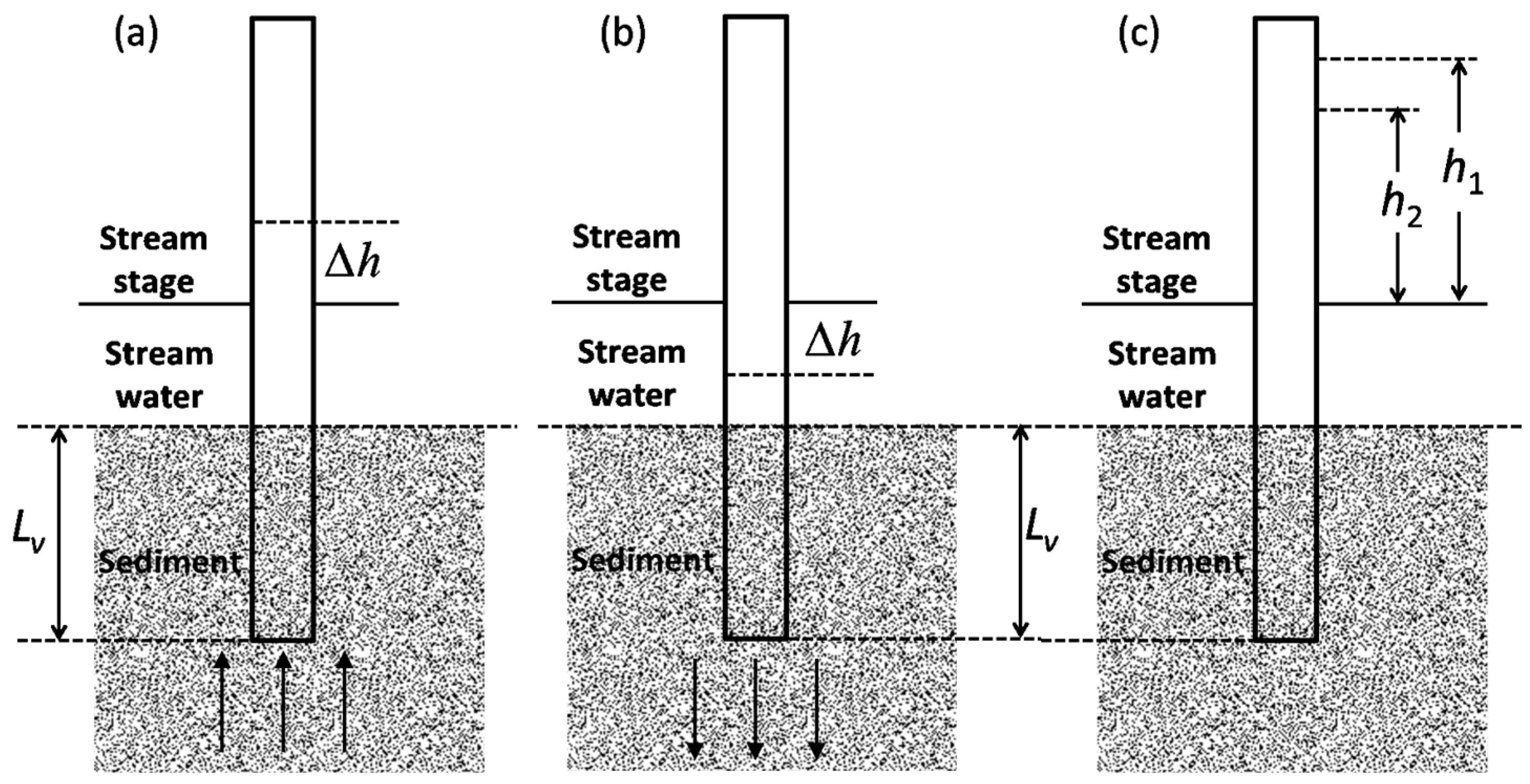
2.2.1. Determination of Vertical Head Gradient

In this study, polyvinyl chloride pipe was used to determine the vertical hydraulic gradient (Figure 2a,b). The transparent pipe was pressed vertically into the submerged streambed slowly to create a sediment column of a certain depth inside the pipe. A hydraulic difference between the stream stage and water level inside the pipe would be recorded after about 16 h to test head gradient [20]. During two test periods, the external conditions changed little. In this study, the pipes used were 160 cm long and their inner diameters were 5.4 cm. The hydraulic head differences were obtained from 31 pipes in July 2015 and 30 pipes in January 2016, respectively. The vertical head gradient (VHG) was calculated with the following equation:

$$VHG=\frac{\Delta h}{L_v}$$

(1)

where L_v is the length of the sediment column inside the pipe and Δh is the difference between the stream stage and the water level inside the pipe. Since Δh is calculated as the subsurface head elevation minus the stage elevation, positive values indicate the potential for upwelling and negative values indicate the potential for downwelling [23].

2.2.2. Determination of Vertical Hydraulic Conductivity

The in situ permeameter test was used to determine the vertical hydraulic conductivity of the sediment columns inside the pipe at each test location after determining VHG (Figure 2c). The test procedure for vertical hydraulic conductivity in streambeds was well documented in previous studies [15,24]. In the present study, the same method was used for the permeameter test. The vertical hydraulic conductivity of sediments can be calculated using the equation proposed by Hvorslev [25]:

$$K_v=\frac{\frac{\mathsf{\pi }D}{11m}+L_v}{t_2-t_1}\ln \left(\frac{h_1}{h_2}\right)$$

(2)

where K_v is the vertical hydraulic conductivity of streambed sediments, m/day; L_v is the length of the sediment column inside the pipe, cm; D is the inner diameter of the pipe, cm; m is the square root of the ratio of the horizontal hydraulic conductivity K_h around the test location to the vertical hydraulic conductivity K_v (i.e., $m=\sqrt{K_h/K_v}$); h₁ and h₂ are the water levels inside the pipe measured, cm; and t₁ and t₂ are the corresponding time, day. In this study, six or 10 potential h₁ and h₂ head measurement pairs were used to calculate the K_v values on the basis of 4–5 head observations at each test point.

Generally, K_h is several times larger than K_v in upper streambed sediments [26]. K_v can be determined via a modified Hvorslev solution when L_v is much larger than D:

$$K_v=\frac{L_v}{t_2-t_1}\ln \left(\frac{h_1}{h_2}\right)$$

(3)

The influences of m and the ratio (L_v/D) of sediment column length (L_v) to the inner diameter (D) of the pipe on the K_v calculation have been discussed by Chen [27]. When 1 < m < 5, if the ratio (L_v/D) is greater than 5, the error of the modified calculation will be less than 5%. In this study, the sediment column length ranged from 38.8 to 48.5 cm in July 2015 and from 38.3 to 46.4 cm in January 2016, respectively; the inner diameter D is 5.4 cm; and the ratio (L_v/D) is greater than 5.

2.2.3. Determination of Vertical Darcian Flux

The Darcian flux (DF) or specific discharge through the streambed can be characterized using the Darcy equation:

$$q_v=K_v\times VHG$$

(4)

where q_v is the potential vertical flux between stream and streambed and its direction is same as that of the vertical hydraulic gradient.

2.2.4. Estimation of Porosity of Streambed Sediments

The volumetric approach was used to determine the porosity of sediments by calculating the sediment bulk and particle density [28]. Wet saturated sediments inside the pipes were oven dried and weighed using a sensitive scale weighing balance to determine the bulk density. The particle density of sediments was assumed to have a value of 2.65 g/cm³ [29]. The calculation formula is as follows:

$$\mathsf{\varphi }=1-\frac{{\mathsf{\rho }}_{bulk}}{{\mathsf{\rho }}_{particle}}$$

(5)

where φ is the porosity of streambed sediments and ${\mathsf{\rho }}_{bulk}$ is the sediment bulk density, g/cm³; ${\mathsf{\rho }}_{particle}$ is the sediment particle density, g/cm³.

Finally, the sediments samples were analyzed with sieving method and assigned into three groups by grain size: silt and clay (<0.075 mm), sand (0.075–2.0 mm), and gravel (>2.0 mm) [14].

3. Results

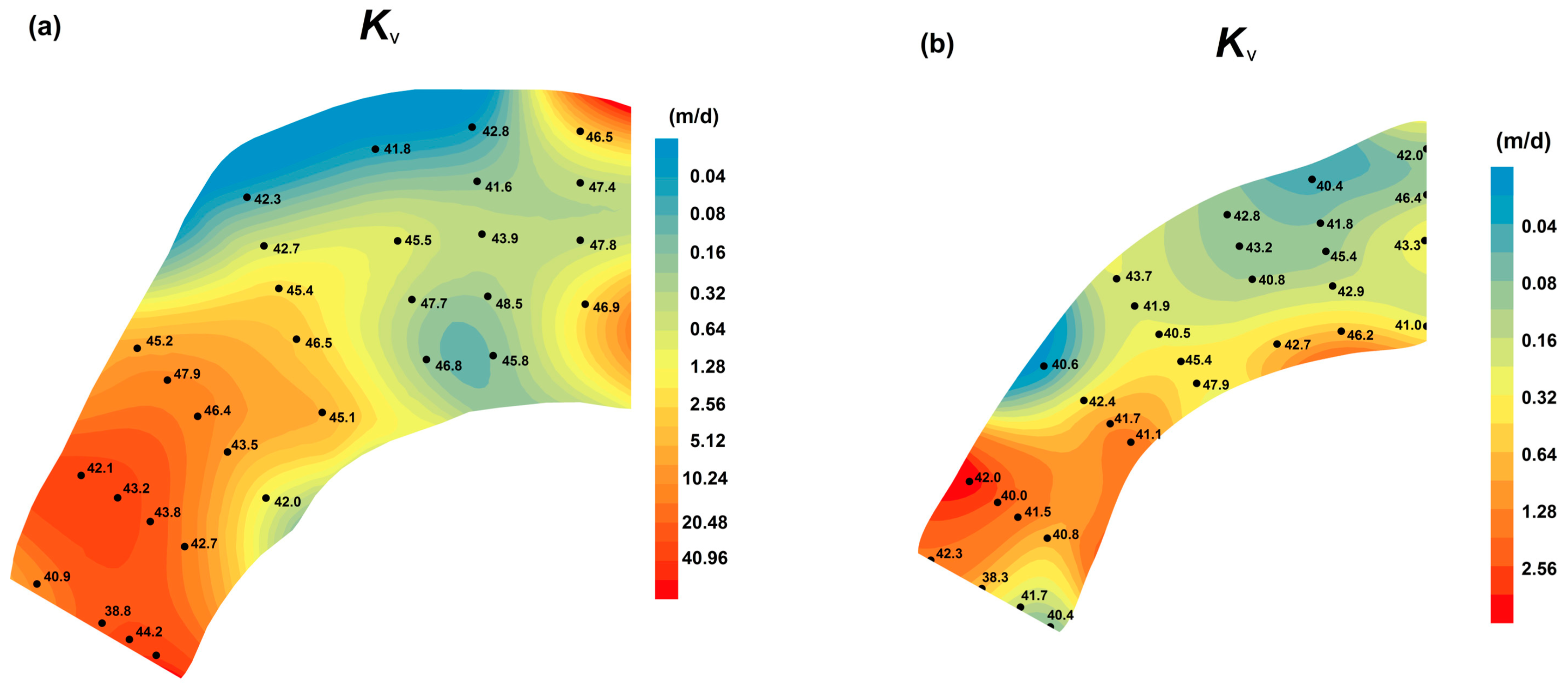
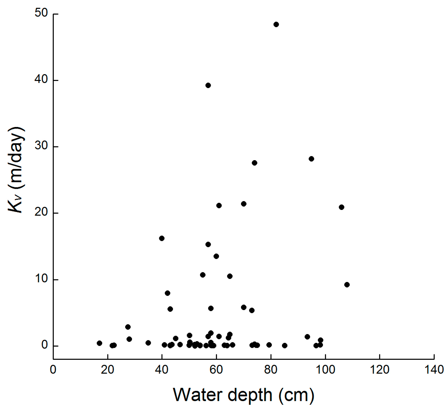
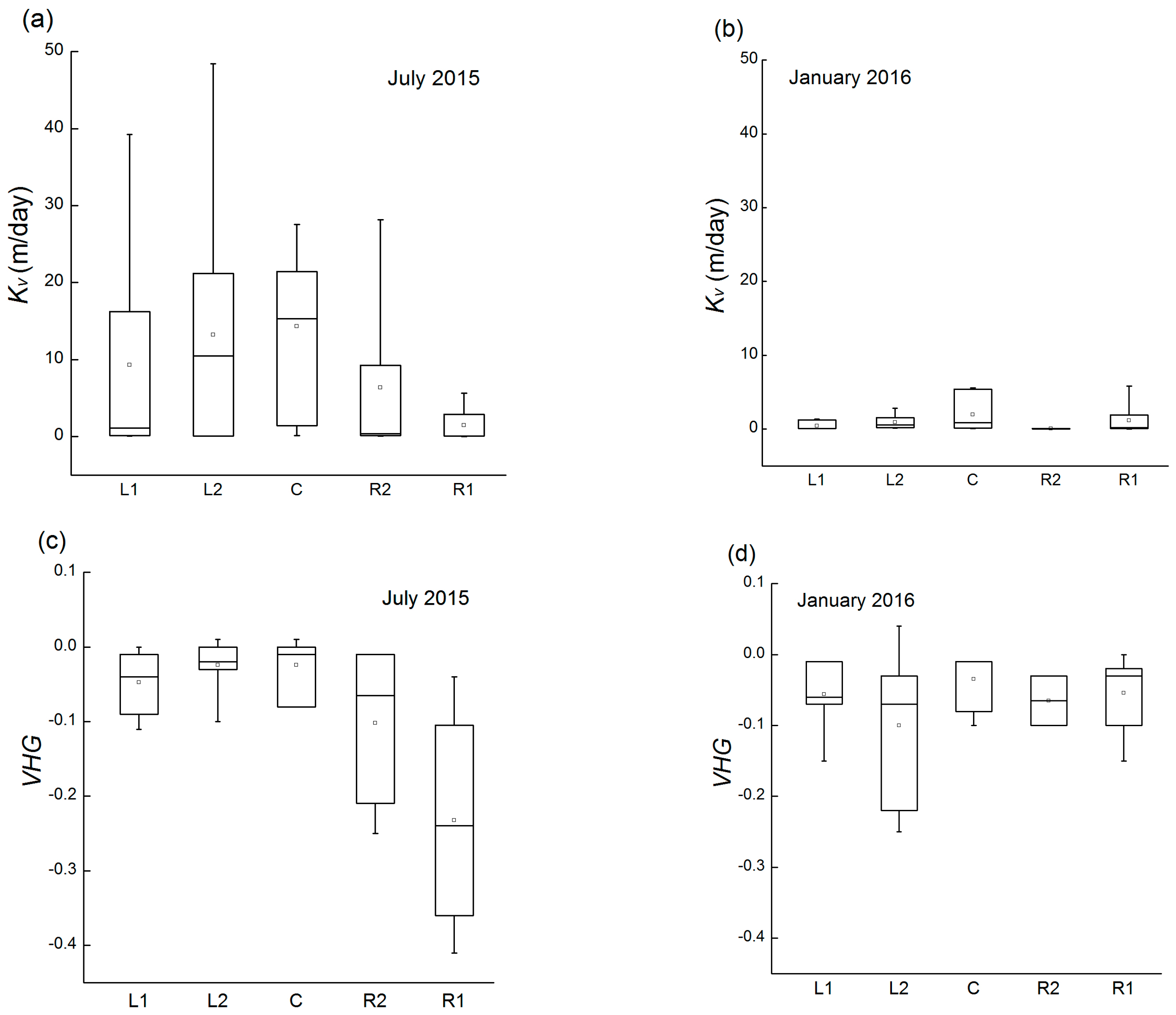
3.1. Vertical Hydraulic Conductivity

The K_v values varied from 0.03 to 48.43 m/day and from 0.01 to 5.82 m/day in July 2015 and January 2016, respectively (

Table 2. Statistics of K_v, K₂₀, VHG, DF, and porosity (φ) during July 2015 and January 2016.

Statistic	Range		Median Value		Average Value		Coefficient of Variation
	July 2015	January 2016	July 2015	January 2016	July 2015	January 2016	July 2015	January 2016
Kv (m/day)	0.03~48.43	0.01~5.82	1.40	0.17	9.20	0.89	1.29	1.62
K20 1 (m/day)	0.02~38.23	0.02~8.55	1.13	0.25	7.45	1.31	1.29	1.62
VHG	−0.41~0.01	−0.25~0.04	−0.03	−0.04	−0.07	−0.06	1.31	1.06
DF (cm/day)	−69.37~62.4	−11.08~6.05	−1.98	−1.41	−6.76	−2.28	1.38	1.46
φ	0.39~0.46	0.39~0.49	0.41	0.41	0.41	0.43	0.04	0.07

Note: ¹ K₂₀ were calculated for a common reference temperature of 20 °C.

). All K_v values of the two test periods spanned over four orders of magnitude, with an average value of 5.11 m/day and a median value of 0.46 m/day. These values and ranges were within the range of K_v values tabulated by Genereux [24], but some large values were out of the range of previous tests in other study sites on the Beiluo River [14]. Shapiro–Wilk normality tests were used to determine whether K_v or lnK_v was normally distributed for either season. The results suggested that neither K_v nor lnK_v was normally distributed at the 95% confidence level, except for lnK_v in January 2016 (N = 31, p = 0.000 for K_v in July 2015; N = 31, p = 0.002 for lnK_v in July 2015; N = 30, p = 0.000 for K_v in January 2016; N = 30, p = 0.318 for lnK_v in January 2016). Previous research showed that streambed hydraulic conductivity was not normally distributed across 101 reaches or that K_v had a lognormal distribution [30,31].

During the two test periods, the high values of K_v were observed in the center of the channel and (Figure 3a,b). Genereux also found higher permeability in the center of the channel with 487 measurement results in West Bear Creek, NC, USA [24]. The present study also suggested that high K_v occurred near the depositional bank. Sebok also found similar results [31].

The interpolation contour plots for both test periods show that high K_v values are downstream of the channel bend, with much higher values in July 2015. Upstream, low K_v values occurred on both sides of the channel in July 2015, but only at the right bank erosion in January 2016. Downstream, high K_v values occurred near the right bank erosion during both test periods (Figure 4a,b). The study also showed an increase in K_v along the channel bend during two both test periods (Figure 5).

The permeability of sediments is affected by the viscosity and density of water which, in turn, varies with the water temperature. K₂₀ were recalculated at a common reference temperature of 20 °C (Table 2). For seasonal comparison, K₂₀ showed a decrease from an arithmetic mean value of 7.45 m/day in July 2015 to 1.31 m/day in January 2016. The Kruskal-Wallis test also indicated significant differences in K_v, K₂₀ between the two test periods (p = 0.004 for K_v; p = 0.022 for K₂₀). Although the water temperature could cause a certain effect on the hydraulic conductivity, the results of statistical tests of K₂₀ and K_v were consistent.

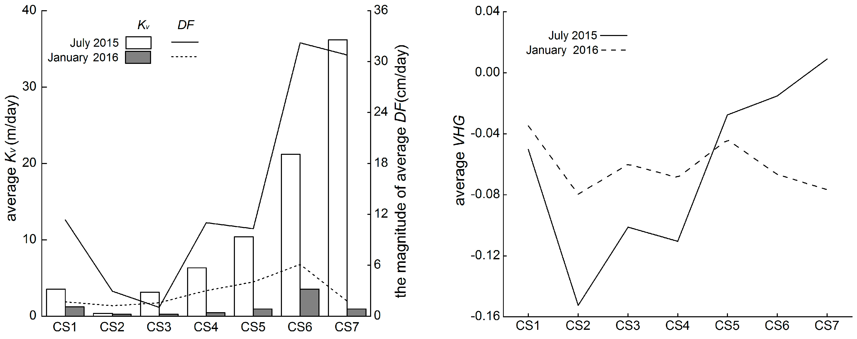
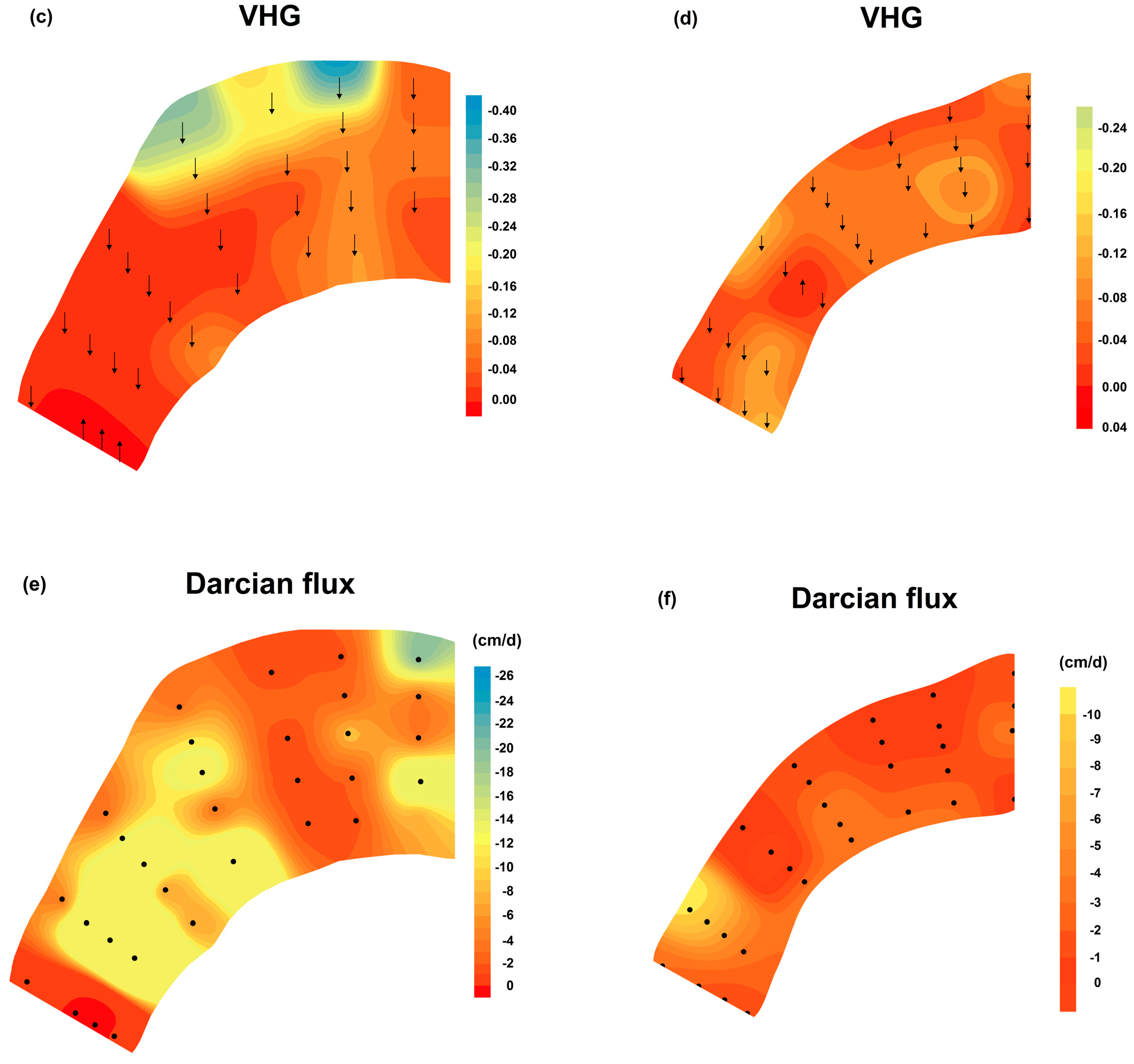
3.2. Vertical Head Gradient

The VHG describes the direction and intensity of the water exchange between the hyporheic zone and the surface or the subterranean zone [32]. The VHG varied between −0.41 and 0.01 and −0.25 and 0.04 in July 2015 and January 2016, respectively (Table 2). Most VHG values were negative, showing downwelling of stream water across the channel during the two test periods (Figure 4c,d). The results of data analysis indicated that high downward VHG values occurred in the upstream part of the channel, with much higher values adjacent to the apex of the bend in July 2015 (Figure 4c). During both test periods, the low downward gradients were in the center of the channel. However, the highest downward gradients occurred near the right bank in July 2015, whereas they occurred near the left bank in January 2016 (Figure 3c,d). In July 2015, the maximum value (0.41) of downward gradient corresponded to a 16 cm hydraulic head difference between the stream stage and the water level inside the pipe.

The VHG showed a greater spatial variability in July 2015 than January 2016 across the study site (Table 2). There was a slight increase in median value of VHG values from July 2015 to January 2016, whereas a higher average VHG value was observed in July 2015. The magnitude of VHG showed an increasing trend after the initial decrease in July 2015, but fluctuated up and down around the average value along the channel (Figure 5). The Kruskal-Wallis test was used to verify whether VHG showed significant differences across the channel or between the two test periods. The results suggested that there was no significant difference between the two test periods (p = 0.557), whereas a significant difference was found between the upstream and downstream sections in July 2015 (p = 0.001 for July 2015, p = 0.856 for January 2016).

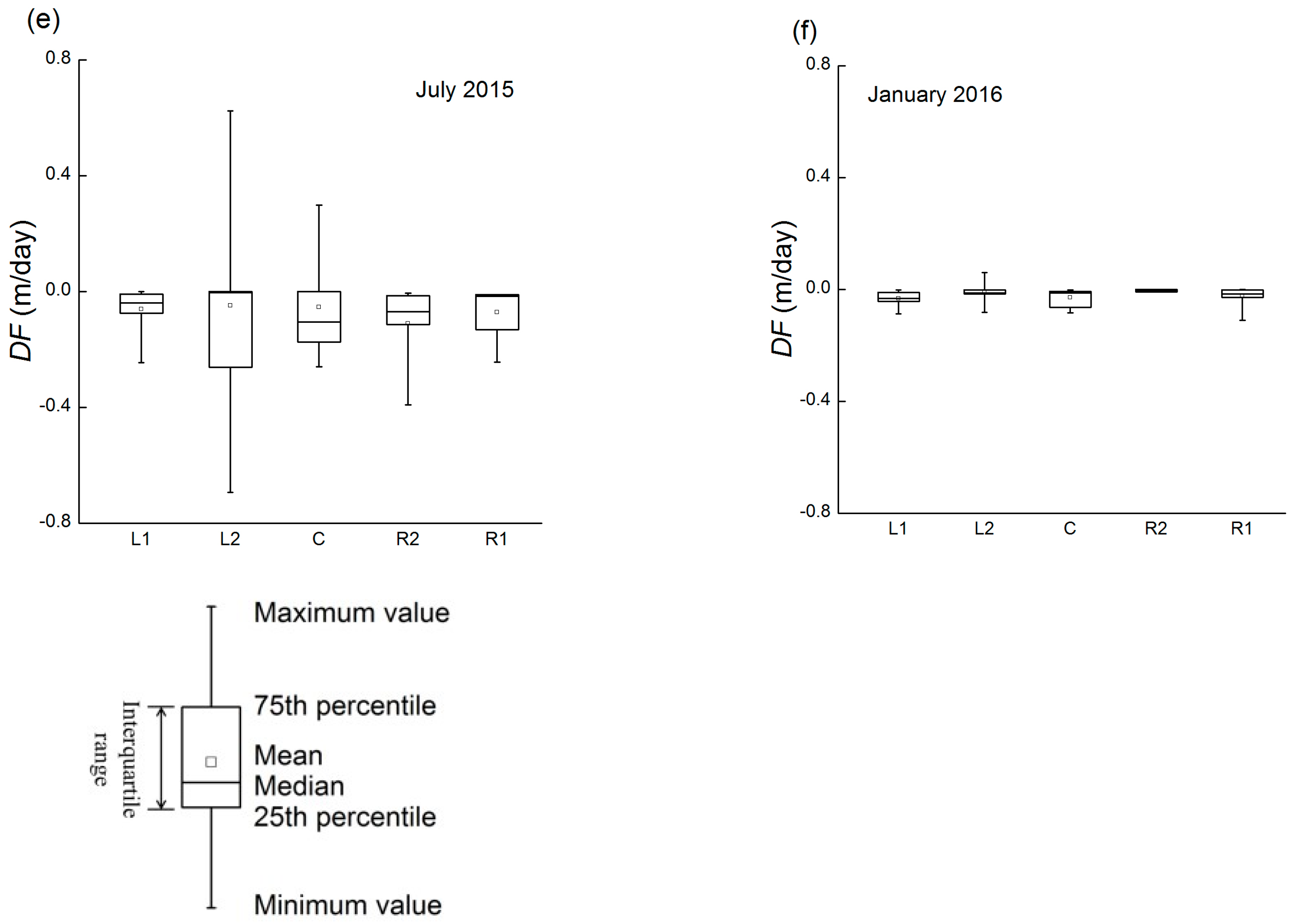
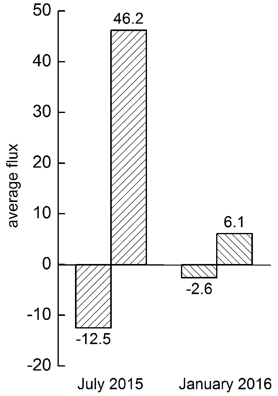
3.3. Vertical Darcian flux

The Darcian flux calculation, employing vertical hydraulic conductivity and the hydraulic gradient, shows the variability in vertical water exchange between the stream and streambed. The vertical Darcian flux ranged from −69.4 to 62.4 cm/day and from −11.1 to 6.1 cm/day in July 2015 and January 2016, respectively (Table 2). Both downwelling and upwelling were observed during the two test periods. The magnitude of Darcian fluxes was greater at the downstream than that at the upstream of the channel during two test periods (Figure 4e,f). There was an increase in the magnitude of flux in the direction of water flow although it decreased initially from CS1 to CS3 in July 2015; and the magnitude of flux increased generally from CS1 to CS6 in January 2016 (Figure 5). The highest values of downwelling were near the deposition left bank and toward the center of the channel during the two periods, but the variations of Darcian flux were complex (Figure 3e,f).

The studied stream section was dominated by downwelling, with upwelling only occurring at four test points (3 for July 2015 and 1 for January 2016) during two test periods (Figure 4c,d). The results of the Kruskal–Wallis test showed no significant difference in Darcian flux between the two test periods, but there was a significant difference in upward fluxes and downward fluxes. The magnitudes of average fluxes were 12.5, 2.6 cm/day for downwelling and 46.2, 6.1 cm/day for upwelling in July 2015 and January 2016, respectively (Figure 6). This difference indicates that the average rate of upwelling was greater than that of downwelling, which is important for stream water and subsurface water.

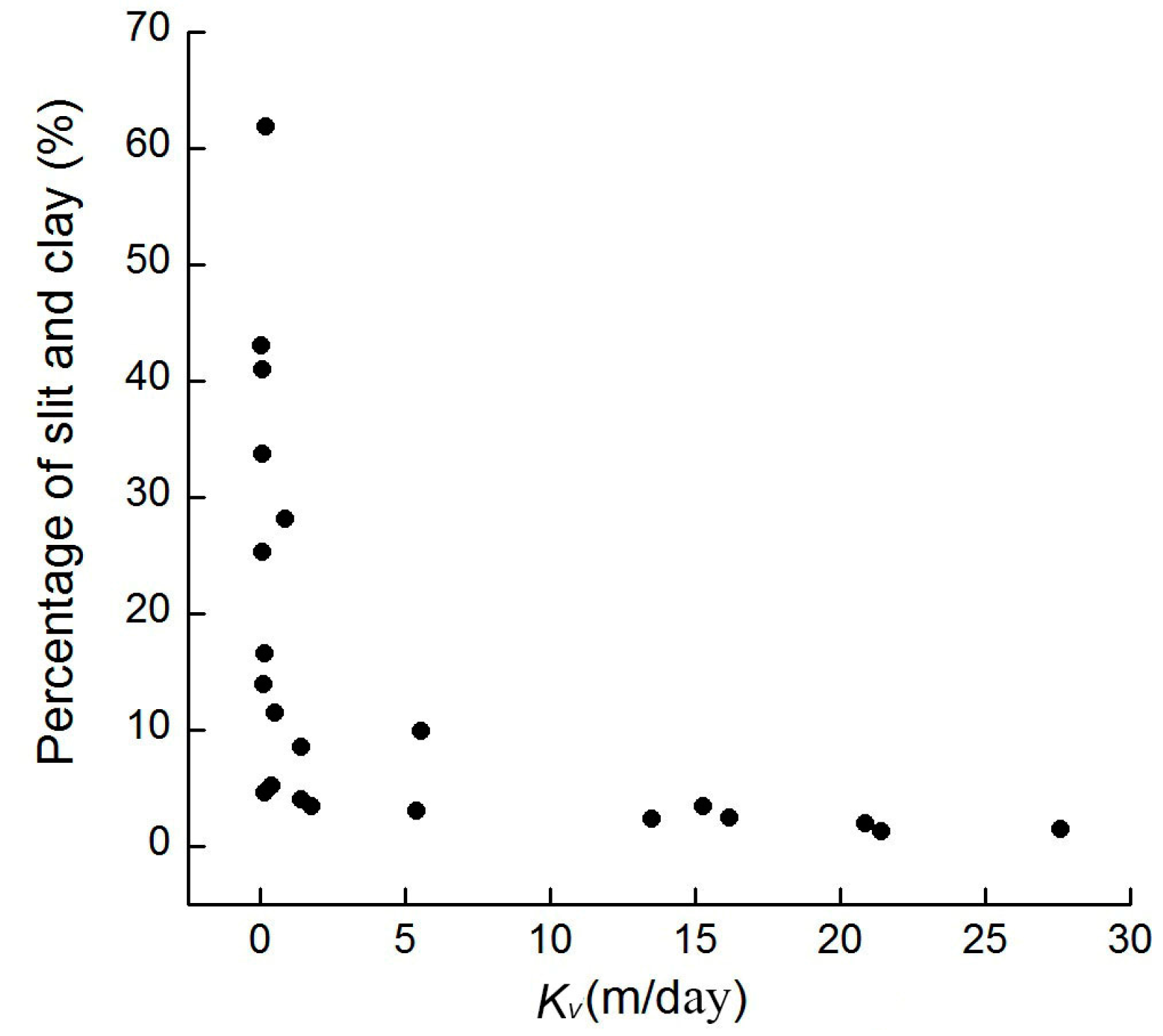
3.4. Sediment Grain Size

Grain size is a key factor in controlling pore size distribution and is the most important characteristic of sediment in determining permeability [33]. The average percentage of sediments with particle sizes of 0.075–2 mm was highest in the center and toward the deposition left bank of the channel, exceeding 90% in July 2015. Inversely, the average percentage of silt and clay was highest at the erosion right bank, exceeding 40% in January 2016 (

Table 3. Sediment grain size distributions at the channel bend during July 2015 and January 2016.

Sediment			July 2015			January 2016
			L and L1	C	R and R1	L and L1	C	R and R1
Particle size	Average percentage (%)	0.075–2 mm (sand)	91.0	91.7	73.1	72.6	78.6	56.2
		<0.075 mm (silt + clay)	3.2	2.4	26.3	25.7	18.3	41.7
	Average median grain size	d50 (mm)	0.18	0.20	0.14	0.15	0.17	0.07

). The median particle size, d₅₀, is an important factor influencing the streambed hydraulic conductivity [34]. Higher average percentages of sand and lower percentages of silt and clay generally generated a larger average median grain size, corresponding to higher K_v values (Table 3, Figure 3a,b). The present study showed high content of slit and clay corresponded to low K_v values (Figure 7), which was consistent with the results by Dong [35]. A negative power relation between the proportion of fine grains and hydraulic conductivity was also found by Miller [36].

4. Discussion

4.1. Porosity

Different relationships between porosity and hydraulic conductivity were obtained: a negative correlation for July 2015 and a positive correlation for January 2016. In general, the hydraulic conductivity could increase with the increasing porosity, but a negative correlation between them also was found under certain distributions and packing arrangements of grain size [28,37,38]. Unlike for K_v, there were no significant differences in porosity, with an equal median value of 0.41 during both test periods (Table 2). Gamage et al. found a general trend of increasing permeability with decreasing percentage of clay size particles at a given porosity [33]. The relationship between hydraulic conductivity and porosity was shown to be related to the interplay between fluid winding through a mass of particles at different microscopic velocities and the shapes and sizes of pores [38].

4.2. Stream Topography

The depositional and erosional process induced by stream flow relating to stream morphology, to a certain extent, might result in the variability of streambed hydraulic conductivity. In this study, lower K_v values were adjacent to the erosional left bank of the channel bend, which is consistent with the observation by Käser [23]. The zone of high K_v values shifted toward the downstream erosional bank in January 2016 (Figure 4b) along the channel bend; a similar result was found by Sebok, who concluded that the lower organic layer could be partially or completely removed because of the increased water velocity [31]. The difference in K_v values in July 2015 is greater than that in January 2016, which may be related to the water velocity and stream geomorphology. The more dynamic environment, mirroring the great water velocity and distinct stream geomorphology, may have resulted in more variable streambed attributes, ultimately causing the hydraulic conductivity to vary [15].

Generally, higher K_v values occurred at lower stream topography, indicating deeper water (Figure 1b,c and Figure 4a,b). Correlation analysis revealed a positive correlation between water depth and K_v for both seasons (Figure 8) and that the correlation was significant at the 95% confidence level (R = 0.287, p = 0.025, N = 61). This finding is consistent with study results obtained by other researchers [15,27]. Larger flow velocity can suspend finer-grained particles and carry them to areas of lower flow velocity while at the same time causing the deeper water and lower stream topography [27].

The hydraulic gradient showing the difference in hydraulic head could be affected by stream slope. The surface water hydraulic head is controlled by the amplitude of undulation in the streambed [21]. The VHG showed different variations along the channel bend during the two test periods (Figure 5). This difference may be related to the amplitude of stream topography. VHG showed a coherent response to stream stage when comparing the whole range of flow conditions [23]. The high downward gradients occurred at the high streambed, which showed advective water flows into the streambed. The alteration of exchange flux direction may be affected by changes in stream topography. The upwelling flux appeared at the CS7 in July 2015 and CS5 in January 2016, respectively. The change in the surface topography affected the velocity field, the head function and the normal vector to the surface, all of which influence the flux calculation [6].

The apex is a special location of the channel bend with low K_v and DF, fine streambed materials and almost stationary water during both test periods. In addition, the average specific discharge and K_v values were higher in July 2015, with a higher curvature than in January 2016. In addition, the specific discharge may be influenced by lateral streambed slope and channel sinuosity [12].

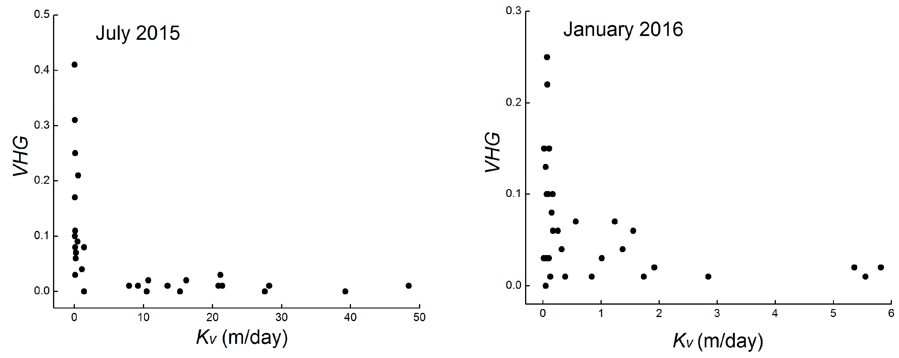
4.3. Correlation of Measured Streambed Attributes

During both test periods, test locations with high K_v values often showed low VHG values, which indicated that VHG was, to some extent, inversely related to K_v (Figure 9). Spearman correlation analysis results suggested that the K_v and VHG values were inversely related at the 95% confidence level (R = −0.485, p = 0.006, N = 31 for July 2015; R = −0.397, p = 0.030, N = 30 for January 2016). This pattern was consistent with the observations by Käser and Sebok [23,31]. Therefore, the variations of Darcian flux were complex and the magnitude of fluxes showed a significant variation across the studied stream section during both test periods.

The extent of exchange between channel and hyporheic water was positively correlated with the streambed hydraulic conductivity [18]. Correlation analysis was used to demonstrate the effect of two variables, K_v and VHG, on the extent of exchange between stream and hyporheic water at the 95% confidence level. The results showed that the Darcian flux was positively and negatively correlated with K_v and VHG, respectively. The correlation coefficients for each test period were 0.685 and −0.308 in July 2015, 0.791 and −0.190 in January 2016, for K_v and VHG, respectively, and the correlation was significant between Darcian flux and K_v (N = 31, p = 0.000; N = 30, p = 0.000) but not between Darcian flux and VHG (N = 31, p = 0.092; N = 30, p = 0.313) during the two test periods. Therefore, this study result supports the conclusion that the intensity of exchange flow is primarily controlled by the streambed hydraulic conductivity. In general, areas of higher seepage rate coincided with areas of higher hydraulic conductivity, and the highest hydraulic gradient values were found only at points with very low hydraulic conductivity [39,40]. This previous result is consistent with the present study. The high K_v values occurred in those zones surrounding the test locations which showed upward VHG (Figure 4a–d). Fine materials may be flushed from the streambed by the upwelling of hyporheic water, whereas coarser particles could be left in the upper streambed [31,36]. This condition further suggests the effect of the hyporheic process on hydraulic conductivity [41].

5. Conclusions

The Darcian fluxes in the hyporheic zone were determined via observations of streambed attributes of vertical hydraulic conductivity (K_v and VHG) at 31 locations in July 2015 and 30 locations in January 2016 along a channel bend. All the streambed attributes—K_v, VHG, and Darcian flux—showed great spatial variability related to the stream morphology and hydrological features in a channel bend, with an especially significant difference in July 2015 due to distinct stream topography.

Vertical Darcian fluxes were mainly dominated by downwelling with high values occurring near the depositional left bend and the downstream of the channel bend, especially in July 2015, and the variations of them were complex. The higher K_v values occurred at the lower streambed elevation with deeper water depth and followed the order stream center > depositional bank > erosional bank. This pattern may result from the distributions of streambed grain size induced by the velocity of stream water and influenced by the stream morphology and topography. The spatial distribution of VHG was inversely related to the distribution of K_v and more easily influenced by the stream topography. These two variables, K_v and VHG, could influence the estimation of Darcian flux. The correlation analysis showed that K_v is the main factor controlling the Darcian flux in the streambed.

While this study observed the variability of vertical Darcian flux between the stream and the hyporheic zone, the lateral water flux in the streambed should not be ignored. Hence, more methods should be employed and additional aspects considered in further studies.

References

1. Hancock, P.J. Human impacts on the stream-groundwater exchange zone. Environ. Manag. 2002, 29, 763–781. [Google Scholar] [CrossRef] [PubMed]
2. Boulton, A.J.; Findlay, S.; Marmonier, P.; Stanley, E.H.; Valett, H.M. The functional significance of the hyporheic zone in streams and rivers. Annu. Rev. Ecol. Syst. 1998, 29, 59–81. [Google Scholar] [CrossRef]
3. Hancock, P.J.; Boulton, A.J.; Humphreys, W.F. Aquifers and hyporheic zones: Towards an ecological understanding of groundwater. Hydrogeol. J. 2005, 13, 98–111. [Google Scholar] [CrossRef]
4. Tonina, D.; Marzadri, A.; Bellin, A. Benthic uptake rate due to hyporheic exchange: The effects of streambed morphology for constant and sinusoidally varying nutrient loads. Water 2015, 7, 398–419. [Google Scholar] [CrossRef]
5. Sophocleous, M. Interactions between groundwater and surface water: The state of the science. Hydrol. J. 2002, 10, 52–67. [Google Scholar]
6. Stonedahl, S.H.; Harvey, J.W.; Packman, A.I. Interactions between hyporheic flow produced by stream meanders, bars, and dunes. Water Resour. Res. 2013, 49, 5450–5461. [Google Scholar] [CrossRef]
7. Hassan, M.A.; Tonina, D.; Beckie, R.D.; Kinnear, M. The effects of discharge and slope on hyporheic flow in step-pool morphologies. Hydrol. Process. 2015, 29, 419–433. [Google Scholar] [CrossRef]
8. Hester, E.T.; Doyle, M.W. In-stream geomorphic structures as drivers of hyporheic exchange. Water Resour. Res. 2008, 44, 893–897. [Google Scholar] [CrossRef]
9. Allen, D.J.; Darling, W.G.; Gooddy, D.C.; Lapworth, D.J.; Newell, A.J.; Williams, A.T. Interaction between groundwater, the hyporheic zone and a Chalk stream: A case study from the River Lambourn, UK. Hydrol. J. 2010, 18, 1125–1141. [Google Scholar]
10. Cardenas, M.B.; Wilson, J.L. Exchange across a sediment–water interface with ambient groundwater discharge. J. Hydrol. 2007, 346, 69–80. [Google Scholar] [CrossRef]
11. Cardenas, M.B. Stream-aquifer interactions and hyporheic exchange in gaining and losing sinuous streams. Water Resour. Res. 2009, 45, 267–272. [Google Scholar] [CrossRef]
12. Cardenas, M.B. A model for lateral hyporheic flow based on valley slope and channel sinuosity. Water Resour. Res. 2009, 45, 206–216. [Google Scholar] [CrossRef]
13. Kalbus, E.; Reinstorf, F.; Schirmer, M. Measuring methods for groundwater-surface water interactions: A review. Hydrol. Earth Syst. 2006, 10, 873–887. [Google Scholar] [CrossRef]
14. Jiang, W.W.; Song, J.X.; Zhang, J.L.; Wang, Y.Y.; Zhang, N.; Zhang, X.H.; Long, Y.Q.; Li, J.X.; Yang, X.G. Spatial variability of streambed vertical hydraulic conductivity and its relation to distinctive stream morphologies in the Beiluo River, Shaanxi Province, China. Hydrol. J. 2015, 23, 1617–1626. [Google Scholar] [CrossRef]
15. Min, L.L.; Yu, J.J.; Liu, C.M.; Zhu, J.T.; Wang, P. The spatial variability of streambed vertical hydraulic conductivity in an intermittent river, northwestern China. Environ. Earth. Sci. 2013, 69, 873–883. [Google Scholar] [CrossRef]
16. Packman, A.I.; Salehin, M. Relative roles of stream flow and sedimentary conditions in controlling hyporheic exchange. Hydrobiologia 2003, 494, 291–297. [Google Scholar] [CrossRef]
17. MacDonald, M.J.; Chu, C.F.; Guilloit, P.P.; Ng, K.M. A generalized Blake-Kozeny equation for multisized spherical particles. AIChE J. 1991, 37, 1583–1588. [Google Scholar] [CrossRef]
18. Edwardson, K.J.; Bowden, W.B.; Dahm, C.; Morrice, J. The hydraulic characteristics and geochemistry of hyporheic and parafluvial zones in Arctic tundra streams, North Slope, Alaska. Adv. Water Resour. 2003, 26, 907–923. [Google Scholar] [CrossRef]
19. Chen, X.H.; Chen, X. Stream water infiltration, bank storage, and storage zone changes due to stream-stage fluctuations. J. Hydrol. 2003, 280, 246–264. [Google Scholar] [CrossRef]
20. Chen, X.H.; Song, J.X.; Cheng, C.; Wang, D.M.; Lackey, S.O. A new method for mapping variability in vertical seepage flux in streambeds. Hydrol. J. 2009, 17, 519–525. [Google Scholar] [CrossRef]
21. Storey, R.G.; Howard, K.W.F.; Williams, D.D. Factors controlling riffle-scale hyporheic exchange flows and their seasonal changes in a gaining stream: A three-dimensional groundwater flow model. Water Resour. Res. 2003, 39, 180–189. [Google Scholar] [CrossRef]
22. Ran, D.C. Water and sediment variation and ecological protection measures in the middle reach of the Yellow River. Resour. Sci. 2006, 28, 93–100. [Google Scholar]
23. Käser, D.H.; Binley, A.; Heathwaite, A.L.; Krause, S. Spatio-temporal variations of hyporheic flow in a riffle-step-pool sequence. Hydrol. Process. 2009, 23, 2138–2149. [Google Scholar] [CrossRef]
24. Genereux, D.P.; Leahy, S.; Mitasova, H.; Kennedy, C.D.; Corbett, D.R. Spatial and temporal variability of streambed hydraulic conductivity in West Bear Creek, North Carolina, USA. J. Hydrol. 2008, 358, 332–353. [Google Scholar] [CrossRef]
25. Hvorslev, M.J. Time Lag and Soil Permeability in Ground-Water Observations; U.S. Army Bulletin: Vicksburg, MS, USA, 1951. [Google Scholar]
26. Chen, X. Streambed hydraulic conductivity for rivers in south-central Nebraska. J. Am. Water Resour. Assoc. 2004, 40, 561–573. [Google Scholar] [CrossRef]
27. Chen, X. Statistical and geostatistical features of streambed hydraulic conductivities in the Platte River, Nebraska. Environ. Geol. 2005, 48, 693–701. [Google Scholar] [CrossRef]
28. Omojola, A.D.; Akinpelu, S.J.; Adesegun, A.M.; Akinyemi, O.D. A Micro Study to Determine Porosity, Hydraulic Conductivity, Permeability and the Discharge Rate of Groundwater in Ondo State Riverbeds, Southwestern Nigeria. Int. J. Geosci. 2014, 5, 1254–1262. [Google Scholar] [CrossRef]
29. Stephens, D.B.; Hsu, K.C.; Prieksat, M.A.; Ankeny, M.D.; Blandford, N.; Roth, T.L.; Kesley, J.A.; Whitworth, J.R. A comparison of estimated and calculated effective porosity. Hydrol. J. 1998, 6, 156–165. [Google Scholar] [CrossRef]
30. Datry, T.; Lamouroux, N.; Thivin, G.; Descloux, S.; Baudoin, J.M. Estimation of sediment hydraulic conductivity in river reaches and its potential use to evaluate streambed clogging. River Res. Appl. 2015, 31, 880–891. [Google Scholar] [CrossRef]
31. Sebok, E.; Duque, C.; Engesgaard, P.; Boegh, E. Spatial variability in streambed hydraulic conductivity of contrasting stream morphologies: Channel bend and straight channel. Hydrol. Process. 2015, 29, 458–472. [Google Scholar] [CrossRef]
32. Mugnai, R.; Sattamini, A.; Ja, A.D.S.; Reguamangia, A.H. A survey of Escherichia coli and Salmonella in the Hyporheic Zone of a subtropical stream: Their bacteriological, physicochemical and environmental relationships. PLoS ONE 2015, 10, 883. [Google Scholar] [CrossRef] [PubMed]
33. Gamage, K.; Screaton, E.; Bekins, B.; Aiello, I. Permeability-porosity relationships of subduction zone sediments. Mar. Geol. 2011, 279, 19–36. [Google Scholar] [CrossRef]
34. Sperry, J.M.; Peirce, J.J. A model for estimating the hydraulic conductivity of granular material based on grain shape, grain size, and porosity. Groundwater 1995, 33, 892–898. [Google Scholar] [CrossRef]
35. Dong, W.H.; Chen, X.H.; Wang, Z.W.; Ou, G.X.; Liu, C. Comparison of vertical hydraulic conductivity in a streambed-point bar system of a gaining stream. J. Hydrol. 2012, 450–451, 9–16. [Google Scholar] [CrossRef]
36. Miller, R.B.; Heeren, D.M.; Fox, G.A.; Halihan, T.; Storm, D.E.; Mittelstet, A.R. The hydraulic conductivity structure of gravel-dominated vadose zones within alluvial floodplains. J. Hydrol. 2014, 513, 229–240. [Google Scholar] [CrossRef]
37. Marion, D.; Nur, A.; Yin, H.; Han, D. Compressional velocity and porosity in sand-clay mixtures. Geophysics 1992, 57, 554–563. [Google Scholar] [CrossRef]
38. Morin, R.H. Negative correlation between porosity and hydraulic conductivity in sand-and-gravel aquifers at Cape Cod, Massachusetts, USA. J. Hydrol. 2006, 316, 43–52. [Google Scholar] [CrossRef]
39. Valett, H.M.; Fisher, S.G.; Grimm, N.B.; Camill, P. Vertical hydrologic exchange and ecological stability of a desert stream ecosystem. Ecology 1994, 75, 548–560. [Google Scholar] [CrossRef]
40. Kennedy, C.D.; Murdoch, L.C.; Genereux, D.P.; Corbett, D.R.; Stone, K.; Pham, P.; Mitasova, H. Comparison of Darcian flux calculations and seepage meter measurements in a sandy streambed in North Carolina, United States. Water Resour. Res. 2010, 46, 5109–5115. [Google Scholar] [CrossRef]
41. Shope, C.L.; Constantz, J.E.; Cooper, C.A.; Reeves, D.M.; Pohll, G.; Mckay, W.A. Influence of a large fluvial island, streambed, and stream bank on surface water-groundwater fluxes and water table dynamics. Water Resour. Res. 2012, 48, 109–119. [Google Scholar] [CrossRef]
Figure 1. (a) Location of the study site within the Beiluo River; (b) streambed topography with test points along the channel bends in July 2015; and (c) streambed topography with test points along the channel bends in January 2016.
Water 09 00170 g001
Figure 2. Measurement setup at each test point: (a) measurement of VHG showing upwelling with upward arrows; (b) measurement of VHG showing downwelling with downward arrows; and (c) measurement of Kv.
Water 09 00170 g002
Figure 3. Box plots of Kv (a,b), VHG (c,d), and DF (e,f) for July 2015 and January 2016.
Water 09 00170 g003aWater 09 00170 g003b
Figure 4. Interpolated contour plots of Kv (a,b), VHG (c,d), and Darcian flux (e,f) in July 2015 (the left plots) and January 2016 (the right plots). (The length of sediments columns has been showed at each test point in plot (a,b); upward and downward arrows in plot (c,d) represent upwelling and downwelling, repectively).
Water 09 00170 g004aWater 09 00170 g004b
Figure 5. Variations of Kv, VHG, and DF along the channel bend in July 2015 and January 2016.
Water 09 00170 g005
Figure 6. Average value of fluxes in July 2015 and January 2016.
Water 09 00170 g006
Figure 7. Relationship of Kv and the percentage of silt and clay.
Water 09 00170 g007
Figure 8. Relationship of Kv and water depth.
Water 09 00170 g008
Figure 9. Relationship between Kv and VHG during the two test periods.
Water 09 00170 g009