1. Introduction
Hydrologic monitoring can provide essential information for flood control, drought relief and the protection of the environment and is the basis for the use and protection of water resources, as well as an important basis for construction, design, planning, and management. As of 2015, China had built 3151 principal hydrological stations, 1313 principal gaging stations, 15,614 precipitation stations, 14,560 water quality stations, 14 evaporation stations, and 16,164 groundwater stations [
1]. Historical and current hydrological data are of great importance for flood control, drought resistance, and the reasonable use of water resources as well as being necessary to make qualitative or quantitative predictions concerning the hydrologic regime of certain regions, water bodies or hydropower stations in future periods. Hydrological work is related to the overall deployment and macro decision-making of the national economy; therefore, forecasting hydrological sequences is of great significance.
Hydrologic data series are also a type of time series. There are many forecasting methods that have been used for hydrologic data series in recent years. The most widely used applications are ensemble empirical mode decomposition (EEMD), Gaussian process regression (GPR), and artificial neural network modeling [
2,
3,
4,
5]. These methods are convenient and direct and often achieve good results in hydrological predictions. The gray forecast method has also been widely used in time series predictions. It places the hydrological research object in an incomplete information system, which is affected by uncertainty factors, usually using the grey system for the input and output, the structure and parameters, or the identification and prediction of a hydrological system [
6,
7]. In addition, seasonal adjustments are often applied to sequences with seasonal trends [
8]. Hydrologic data have a seasonal trend; therefore, the seasonal adjustment method (SAM) is often used for hydrological data prediction. In addition, the use of hybrid models to forecast hydrologic data series is very popular because they combine several different models into a hybrid model, and they are widely used in various fields of prediction and analysis [
9,
10,
11,
12,
13].
Due to the importance of hydrology research, many methods have been developed. Wang has used the extreme learning machine (ELM), Ljung-Box Q-test (LBQ), and the seasonal auto-regressive integrated moving average (SARIMA) model to forecast wind speed, which achieved ideal results [
14]. Reasonably good results have been achieved via the process of decomposing the data with EWL, calculating the correlation of the input value with the LACF method, and then forecasting the data. Altava-Ortiz et al. [
15] researched heavy rainfall events based on the mesoscale meteorological model (MM5) and the analogous method. To improve studies concerning rainfall, Yu [
16] selected the ensemble numerical weather prediction (NWP) model. For quantitative precipitation forecasting, an analog sorting approach was chosen by Obled [
17]. In addition, the analog method was used for statistical precipitation downscaling [
18]. Gholami et al. [
19] used dendrochronology and an artificial neural network (ANN) to evaluate groundwater level fluctuations, which rendered a high degree of accuracy and efficiency in the simulation of groundwater levels. These studies all have their own advantages and have achieved different levels of prediction. However, they also have their limitations. These methods cannot always obtain a satisfactory forecasting accuracy when the data simultaneously shows nonlinearity and nonstability.
The primary challenge for this paper is to fully extract information to better fit the original data series. Time series often have obvious seasonal trends and are unstable. In this case, the use of a single seasonal adjustment or a neural network is not sufficient to fully extract the information in the series. We need to find a way to fully decompose the series and then to extract the trend terms and the error terms from the decomposition results. In the decomposition method, we need to deal with nonlinear and unstable data. In addition, in the following forecast, we need to fully extract the linear part of the series. This process requires repeated attempts.
EEMD can deal well with nonlinear and nonstationary data series and can extract useful information from the data by decomposing the original data series. In Wang’s article [
20], the autoregressive integrated moving average (ARIMA) model coupled with EEMD is presented to forecast annual runoff time series. The results indicate that EEMD can effectively enhance the forecasting accuracy. The radial basis function neural networks (RBFN) model is widely used in time series analysis and can effectively forecast data series because it has good generalization ability. The Support Vector function (SVM) model can effectively avoid the local minima problem and has good generalization ability. These three models are widely used when dealing with nonlinear and non-stationary data series. Model choices have a large influence on the prediction results, and the selection of parameters will determine a model’s quality [
21].
Neural networks are often used for hydrologic forecasting. A hybrid model coupled with singular spectrum analysis was applied to daily rainfall predictions by Chau and produced good results [
22]. In addition, neural networks are often used for data preprocessing [
23]. Neural networks have been widely used in many fields in recent years and have achieved good results. Based on EEMD, RBFN, and SVM, a hybrid model, EEMD–RBFN–SVM, was proposed to settle the hydrologic problem. The precipitation data from the Qinghai Yushu Tibetan Autonomous Region, which has obvious seasonality and nonstability, were used as an illustrative example to evaluate the performance of the EEMD–RBFN–SVM model. In this paper, first, the original data series were decomposed with EEMD, and a dataset was obtained. Second, the decomposed series were forecast with RBFN to obtain the prediction error. Finally, the errors were corrected with SVM to obtain the final prediction results. The results show that the hybrid model makes full use of the useful information in the original data series and forecasts the precipitation data series effectively.
The structure of the paper is as follows.
Section 2 introduces the respective models, puts forward the hybrid model, and describes the test indicators for the model.
Section 3 provides the case analysis, in which the effectiveness of our proposed hybrid model is verified based on the precipitation in the Yushu Tibetan Autonomous Region of the Qinghai Province.
Section 4 offers a comparison of the models. The EEMD–RBFN–SVM model numerically outperformed the following models: the hybrid EEMD and RBFN (EEMD–RBFN) model, the RBFN model, the hybrid SAM model, the ESM model, and the RBFN (SAM–ESM–RBFN) model. Finally,
Section 5 summarizes the results.
2. The Proposed Approach
This section presents the EEMD–RBFN–SVM model. First, the EEMD, RBFN, and SVM methods are briefly introduced and the approach of the EEMD–RBFN–SVM model is presented. In addition, the predictive performance evaluation indexes are introduced.
2.1. Ensemble Empirical Mode Decomposition (EEMD)
2.1.1. Empirical Mode Decomposition (EMD)
As a processing method of nonstationary and nonlinear data series, the EMD is most suitable. It was proposed by Huang [
24] in 1998 and 1999 based on a profound study concerning the concept of instantaneous frequency. The essence of the method is to convert an irregular signal into a stationary signal process via continuously eliminating the average envelope of the sequence to make the sequence smooth. After the EMD decomposition, the irregular signal sequence is disaggregated into several intrinsic mode functions, IMFs, and each IMF represents the information of different scales of the original time series. Via the EMD decomposition, the original sequence can be decomposed into a number of IMFs and residuals,
.
The primary properties of the EMD method include adaptability, orthogonality, completeness, and the modulation characteristic of the IMF component. Adaptability reflects that the series can be resolved according to the information of the signal itself, and the basis function comes directly from the signal. Orthogonality means that each component is orthogonal to each other, a result of the decomposition of the signal. Completeness means that the original sequence, which is decomposed via the EMD method, can be restored by the addition of each component, that is, the information is not lost through the decomposition. Finally, the EMD method also has the modulation characteristic of the IMF component [
25].
EMD has obvious advantages when dealing with nonstationary and nonlinear data; therefore, it is widely used for modal parameter identification in oceans, celestial bodies, hydrology, and large-scale civil engineering structures. However, when the EMD method decomposes an unstable data series, the mixed mode overlap phenomenon often appears. This phenomenon is caused by disruptions in the signal, which can lead to confusion in the time-frequency distribution, undermining the physical meaning of the IMF and affecting the accuracy of the decomposition results. Focusing on the deficiencies of EMD, Wu et al. added prediction theory to the EMD decomposition process via the addition of a certain proportion of white noise to the original data to aid decomposition, that is, EEMD. Below is an introduction to EEMD.
2.1.2. Ensemble Empirical Mode Decomposition (EEMD)
The EEMD method was proposed by Wu and Huang [
26]. According to this method, a signal can be made continuous by adding Gaussian white noise to it, and this can be achieved thanks to the uniform distributive nature of Gaussian white noise. Signals in different scale regions will be automatically mapped to appropriate scales, which are related to the white background noise. Finally, the joined white noises are offset from each other by calculating their average. This process solves the mode mixing problem, which is caused by the interval signal. This is the basic principle of the EEMD method. The specific process of the EEMD method is as follows:
- (1)
Add a white noise sequence of a given amplitude to the original sequence.
- (2)
Decompose the mixed signal with the added white noise into IMF1 using the EMD procedure.
- (3)
Add white noise sequences of the same amplitude to the original sequence without IMF1. Then, decompose the sequence using EMD to obtain IMF2.
- (4)
Repeat the above steps until the different IMFs and the final trend item RES are obtained.
- (5)
The final solution is the ensemble mean of the corresponding IMFs.
The intrinsic mode function, IMF, needs to meet the following two conditions:
- (1)
Over the entire signal length, the number of extreme points and the zero crossing must be equal to or at least one of the differences.
- (2)
At any moment, the average value of the upper envelope defined by the maximum value point and the lower envelope defined by the minimum point is zero [
27].
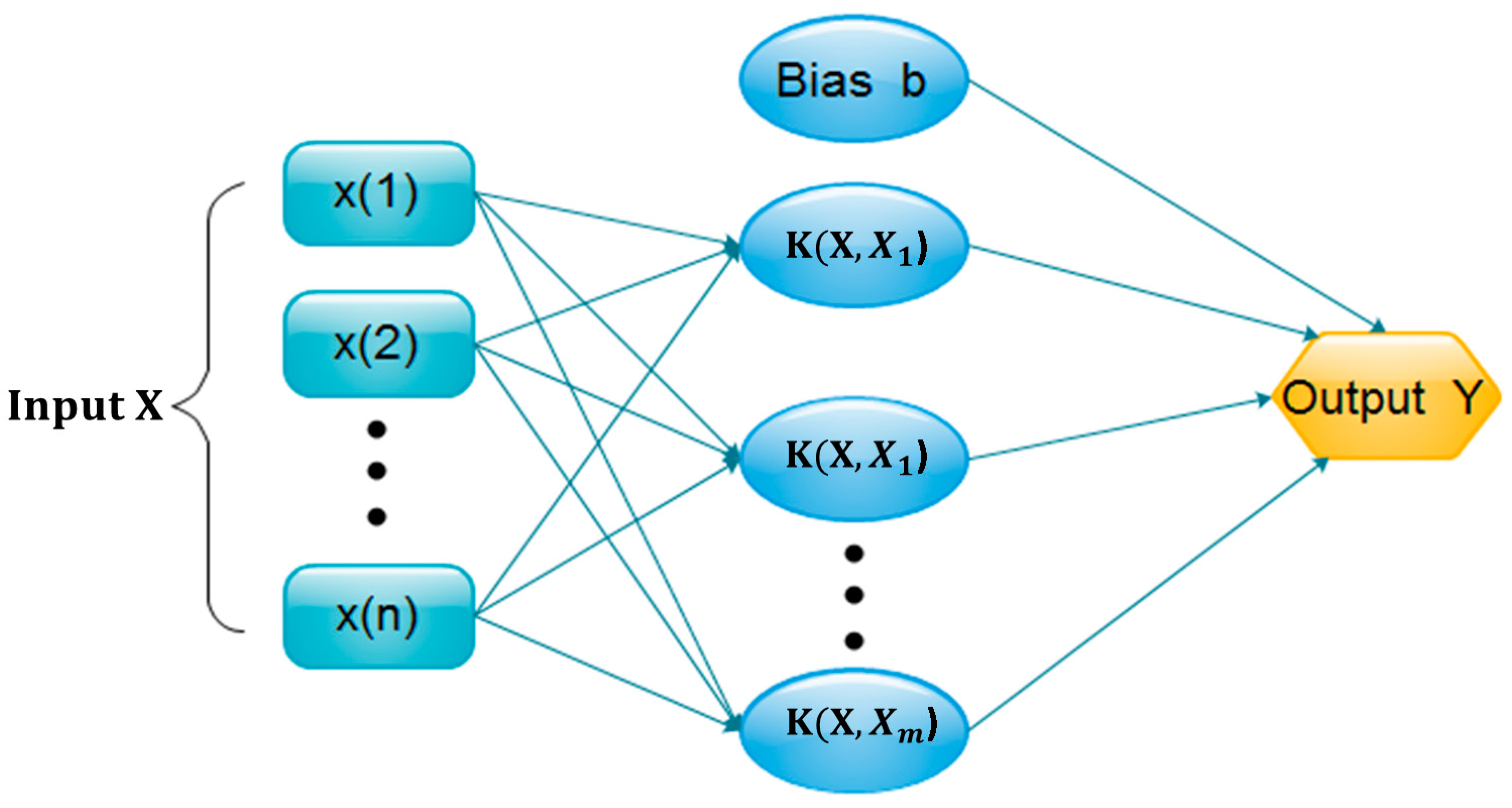
2.2. Radial Basis Function Neural Networks (RBFN)
The RBFN method is a type of three–layer forward network. Broombead and Lowe were the first to apply RBFN to the design of a neural network. The structure of RBFN is similar to a multilayer forward network, and its input layer is composed of the signal source node, the second layer is the hidden layer, and the number of hidden units depends on the description of the problem. The transformation function RBF() is a nonnegative and nonlinear function of the radial symmetry of the center point. The third layer is the output layer, which responds to the input mode. The transformation from the input space to the hidden layer space is nonlinear, and the output layer space transformation from the hidden layer space is linear. It is a static network, and the function approximation theory is consistent with only the best approximation point. The structure of the network is shown in
Figure 1.
Here,
is the input of the RBFN values, W is the output weight matrix, Y is the output, and
is the activation function. The RBFN neurons in the output layer are usually just represented via simple linear weighting [
28]. Typical basis functions include the following:
- (1)
thin-plate-spline functions:
- (2)
multiquadratic functions:
- (3)
multiquadratic inverse functions:
- (4)
In the above formulas,
r represents the Euclidean distance of the data point x to the center of the base function and
β is the extension constant. The Gaussian function is the most commonly used basis function of the radial basis function. The basic idea of RBFN is as follows.
- (1)
Using RBF as the “base” of the hidden units, the hidden layer space is formed, and the input vector is directly mapped to the hidden space.
- (2)
When the central point of the RBN is determined, the mapping relationship is also determined.
- (3)
The mapping of the hidden layer space to the output space is linear.
RBFN has a faster learning speed than the back-propagation (BP) network, and its function approximation ability, model recognition, and classification ability are also better than those of the BP network [
29,
30]. The BP network is a type of global approximation network that makes a corresponding parameter adjustment for each input and output data. However, RBFN is a type of local approximation network. The output of the network is determined only by a small number of neurons. The neurons of the BP neural network have a large visible input region because this method uses the sigmoid() function as its activation function, while RBFN uses the radial basis function and generally the Gaussian function as its activation function, which makes the neurons in the input control area very small and therefore requires additional radial basis neurons. Because the generalization ability of RBFN is better than that of the BP network, the RBF network has been widely used in many fields of research [
31,
32].
2.3. Support Vector Machine (SVM)
SVM was proposed by Vapnik [
33] for applications to the classification of data and text, system modeling and prediction, pattern recognition, anomaly detection, and time series prediction, similar to that of the multilayer perceptron network and the Radial Basis Function Network. SVM has versatility, robustness, effectiveness, and computational advantages, such as being simple. This method solves practical problems using only a simple optimization technique, and has obtained good results. The system structure is shown in
Figure 2.
is the kernel function, and the commonly used kernel functions are listed below.
- (1)
- (2)
Polynomial kernel function:
- (3)
Radial basis kernel function:
- (4)
Two layer perceptron kernel function:
The most widely used of these kernel functions is the radial basis kernel function, which is suitable for large or small samples and high or low dimensions. In this paper, the radial basis kernel function was chosen as the kernel function.
The basic idea of SVM is that, based on the statistical learning theory, via nonlinear mapping and adopting the structural risk minimization principle, it can map a low dimensional space and linearly inseparable data samples into a high dimensional space, so that the data become linear and separable, and then, it places the data in the high dimensional space for classification and prediction. The SVM algorithm can effectively avoid the local extremum problem and, in the case of limited sample information, seek the best value between the model complexity and learning ability, therefore improving its generalization ability. In this study, the SVM method is used to correct the error term, and the operation process [
28] is as follows.
- (1)
Data preprocessing. The SVM algorithm for data normalization preprocessing methods, uses the mapminmax function to implement, the normalized mapping as follows:
In the formula,
,
. Via normalizing, the original data are normalized to the [0, 1] range.
- (2)
Cross validation is performed to select the best parameters of the regression, c and g, where c is the penalty parameter of svmtrain and g is the kernel function parameter.
- (3)
Use the best parameters obtained in step 2 to train the SVM.
- (4)
Fitting prediction. Use the trained SVM to predict the original data sequence.
The process of selecting the optimal parameters via cross validation is as follows [
28]. First, select values for c and g in a certain range. For the selected c and g, the training set is used as the original data set to obtain the classification accuracy of the training set validation based on the values of the selected c and g via the k-CV method. Finally, the c and g that generate the highest classification accuracy are selected as the best parameters. When there are multiple sets of c and g that meet the above requirements, the set of c and g with the minimum c parameter shall be selected as the best set of parameters. If there is more than one g corresponding to the minimum c parameter, the first set of c and g found shall be selected as the best parameters. Regression is achieved using SVMcgForRegress.m.
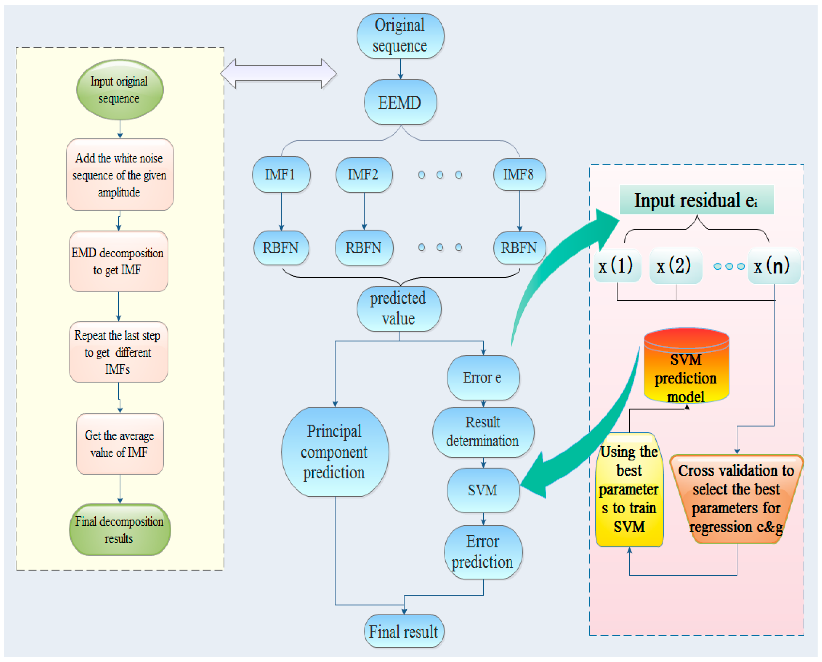
2.4. The Proposed Hybrid Model
To solve the short-term forecasting problem of hydrological data, a hybrid model based on EEMD, RBFN, and SVM is proposed, namely, the EEMD–RBFN–SVM model. EEMD is used to decompose the original sequence, and the decomposition results are predicted by RBFN. Finally, SVM is used to correct the error term. The specific algorithm is as follows.
- Step 1:
Decomposition of the original sequence. The original data sequence is decomposed into eight sequences IMF1, IMF2…IMF8 by EEMD.
- Step 2:
The prediction of the intrinsic mode function. Using RBFN to predict the decomposition of the eight sequences, we obtain eight prediction values IMF1’, IMF2’…IMF8’.
- Step 3:
Error correction. Using the results of steps one and two to get the error term , the SVM method is used to predict the error term .
- Step 4:
Prediction of the original sequence. The predicted value of the original sequence is obtained from the prediction of the intrinsic mode function and the correction of the error term.
The operation flow is shown in
Figure 3.
2.5. Predictive Performance Evaluation Index
To confirm that the proposed hybrid model is better than other models, we selected four evaluation indexes: RMSE, MAE, MaxAE, and the Pearson correlation. They are defined as follows.
Root mean square error, RMSE:
Mean Absolute Error, MAE:
Maximum absolute percent error, MaxAE:
When the values of the indices are smaller, the forecast performance is better.
The Pearson correlation is judged by the size of the Pearson correlation coefficient. The Pearson correlation coefficient, also known as the Pearson product moment correlation coefficient, is a linear correlation coefficient. It is a statistic used to reflect the degree of the linear correlation between two variables. Its expression is as follows:
Above, r is the Pearson correlation coefficient; n is the sample size; , and , are two variables’ observed values and means, respectively; and and are the variances of the two variables, respectively; A higher absolute value of r indicates a stronger correlation between the two groups of variables.
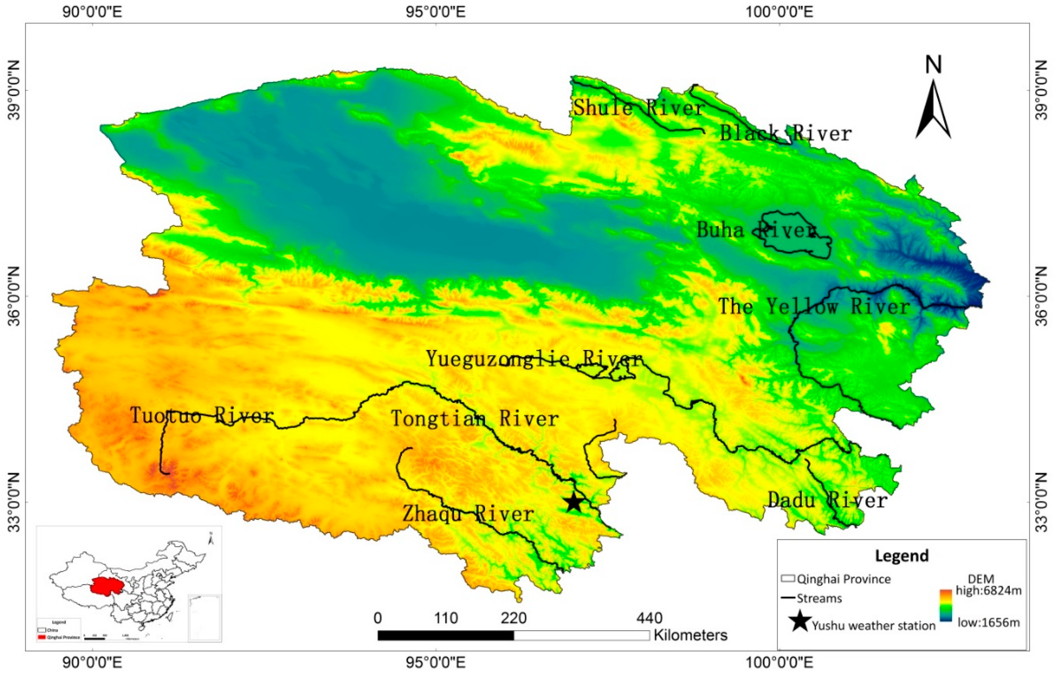
3. Case Study
The monthly precipitation data from the Yushu Tibetan Autonomous Region of the Qinghai Province were collected to examine the hybrid model. Yushu is located at the headwaters of the Yangtze, Yellow, and Lancang Rivers, southwest of the hinterland of the Qinghai-Tibet Plateau in the Qinghai Province, at an average altitude of 4200 m. The location of Yushu is shown in
Figure 4.
Yushu is a meteorological disaster prone area, which makes its weather forecasts very important. The Yangtze, Yellow River, and Lancang Rivers all originate in this locale. Its climate is cold, there is no difference between the four seasons, and the annual rainfall is approximately 520 mm. Due to its special geographical position, precipitation data forecasting is indeed critical in this case.
Because the precipitation in Yushu in recent years has not changed much compared to previous years, we selected data for Yushu from January 1953 to December 2008 to establish the model. The data are shown in
Figure 5. From the trend graph in
Figure 5, we can see that the precipitation data are obviously nonstationary and nonlinear.
3.1. Decomposition of the Original Sequence
EEMD is often used to decompose nonlinear and nonstationary signals into a few intrinsic mode functions (IMFs). In this study, we adopted the EEMD method, and the original series of the precipitation data were decomposed into eight independent IMFs (illustrated in
Figure 6). The decomposition of the results was processed separately so that the trend characteristics of the original sequence could be forecasted and processed well.
3.2. Prediction of the Intrinsic Mode Function
Via the observation and analysis of the eight intrinsic mode function sequences, we concluded that they were nonlinear; therefore, RBFN was used in this study. The RBF is not only simple in structure and for training but also fast in learning and can effectively approximate any nonlinear function. Therefore, in this study, RBFN was selected to predict the eight sequences. The previous 12 data points were used as input data after considering the cycle effects of the monthly precipitation data, that is, the 13th data point is predicted by the 1st to 12th data points, the 14th data point is predicted by the 2nd to 13th data, and so on. In addition, the previous 600 data points were selected as the training set, and the 601st to the 660th data points as the test set to obtain 60 predictive values. Finally, the eight sequence predictions were obtained and merged to produce the predicted value of the original sequence.
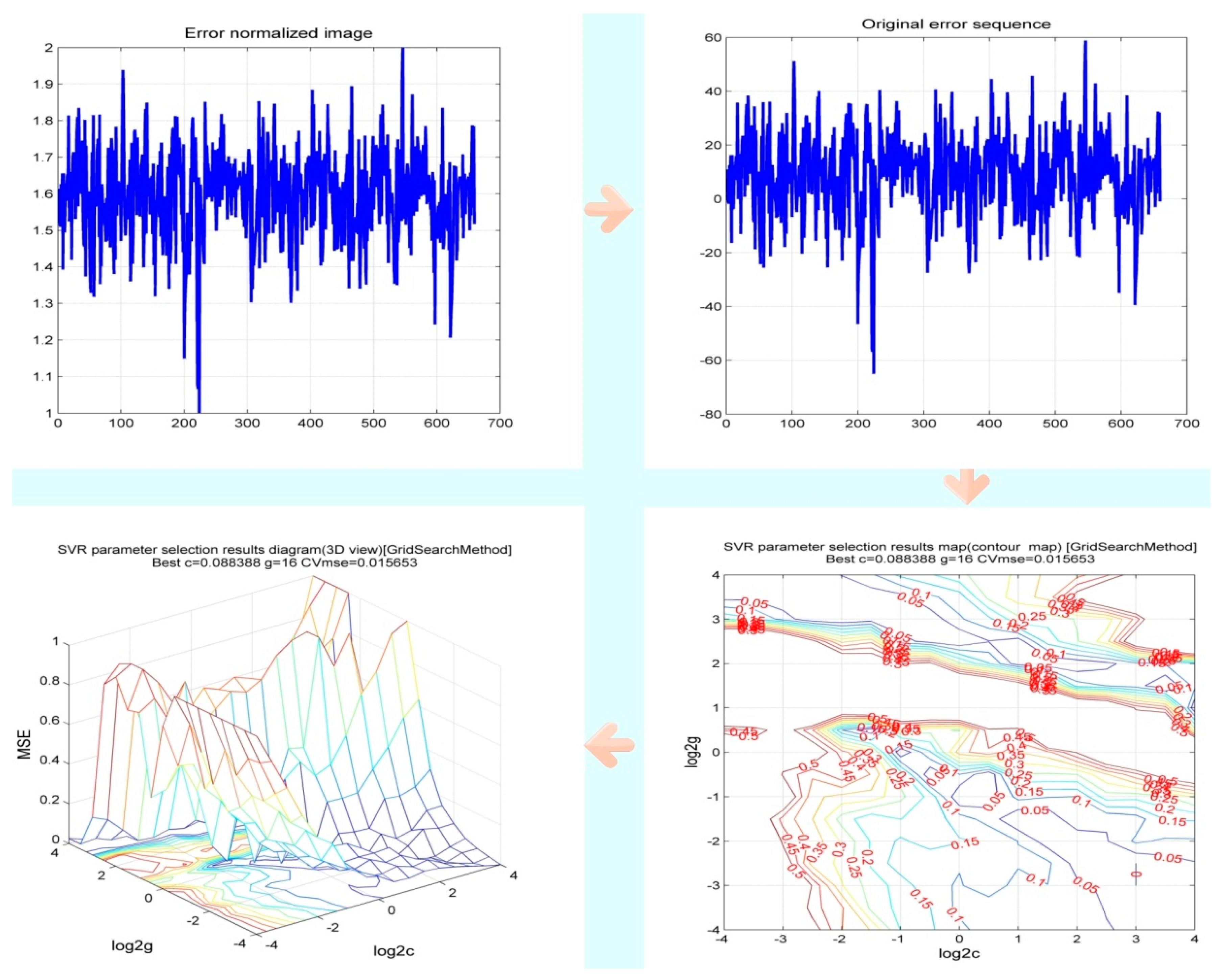
3.3. Error Correction
The prediction of the original sequence will produce a certain error. This study used the SVM method to predict the error term. Using the 1st to the 659th data points as the input values and the 2nd to the 660th data points as the output value, we obtained 60 error terms (
). Cross validation was employed to optimize the parameters, and the final optimization results are g = 16, and c = 0.088388 (c is the penalty parameter of svmtrain, and g is the kernel function parameter). The process is shown in
Figure 7. Finally, the predicted value of the original sequence
was obtained by combining the prediction results of RBFN.
3.4. Prediction of the Original Sequence
Via the decomposition of the original sequence, eight decomposition results were obtained, and these decomposition results were predicted by RBFN. The error term was obtained and modified by SVM, and the final predicted value was then obtained. The forecasting results of the different models are revealed in
Figure 8. The results show that the hybrid design concept can combine different advantages from each individual model.
4. Comparison and Discussion
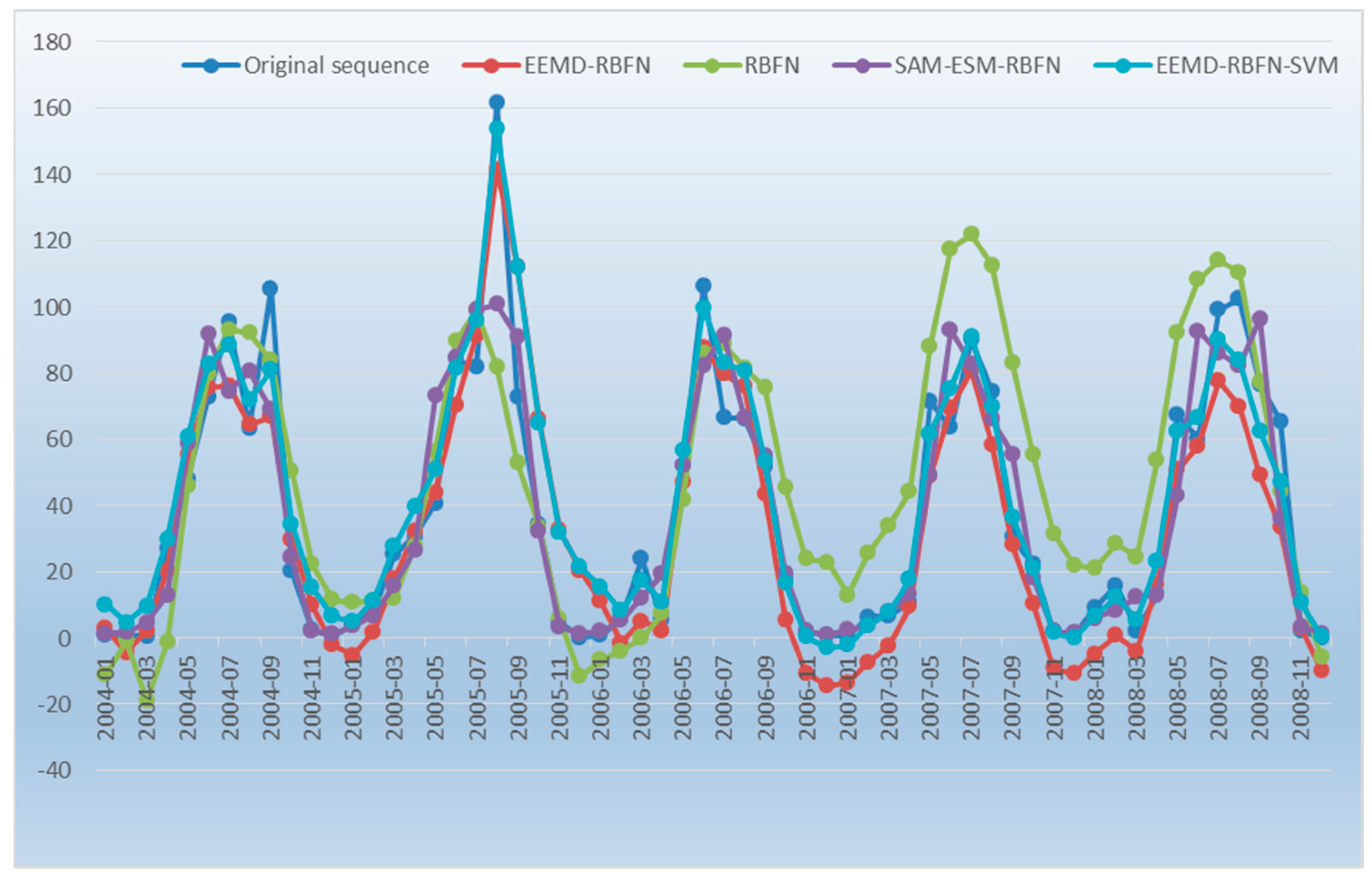
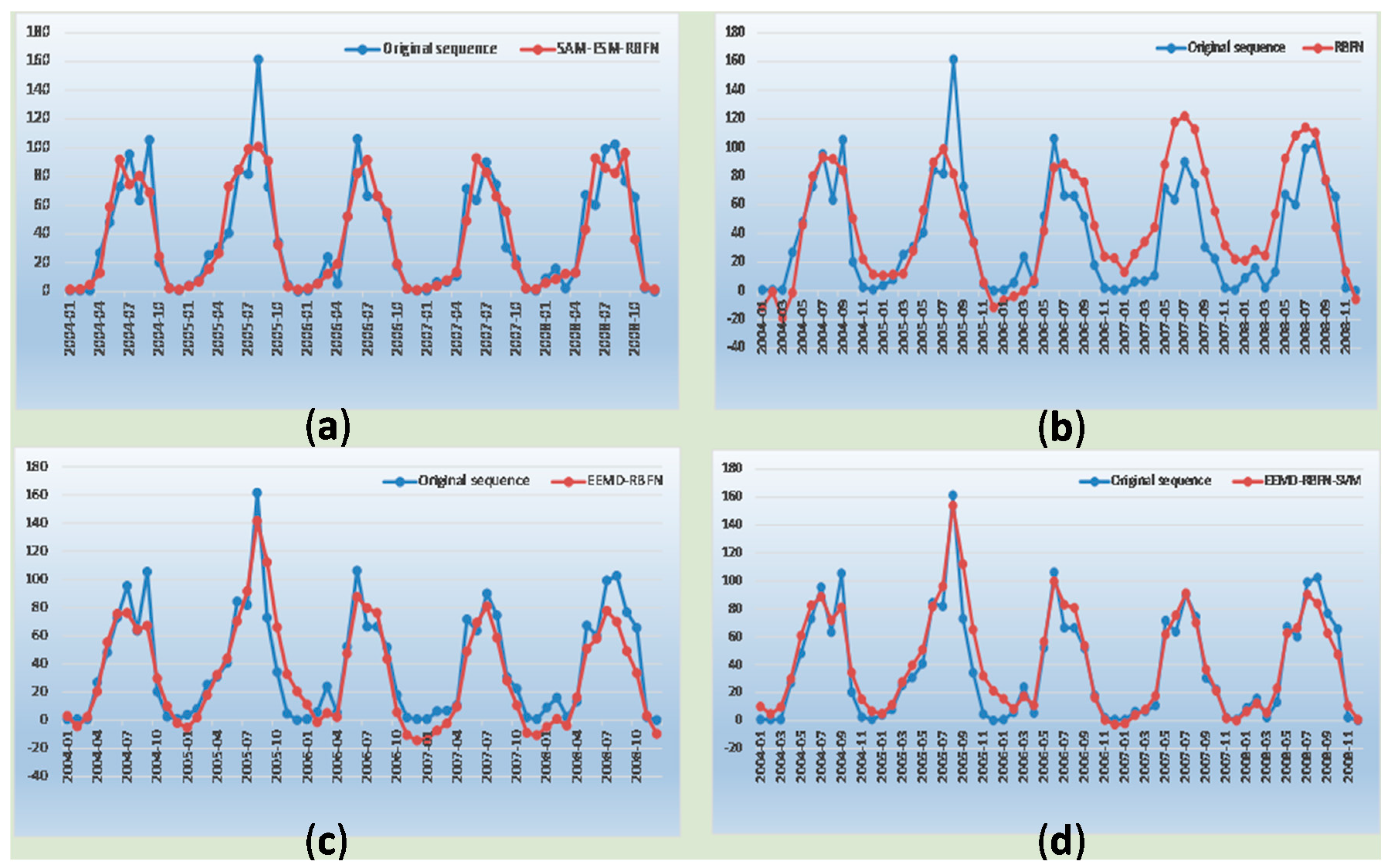
To confirm the model’s superiority, it is necessary to build other models to compare to the proposed model, that is, the RBFN, EEMD–RBFN and SAM–ESM–RBFN models. RBFN is widely used in time series analysis, nonlinear function approximation, and pattern recognition due to its fast learning speed and good generalization ability. RBFN is often used to solve problems in hydrology and meteorology, and the EEMD–RBFN model is a further improvement of RBFN. Via the decomposition of EEMD, additional morphological characteristics of each model can be taken into account; therefore, it is widely used in a variety of meteorological data processing methods. The hybrid SAM–ESM–RBFN model has achieved good results when solving weather problems such as wind speed. In addition, we used several common methods to deal with the data, such as the hybrid EEMD–ARIMA–RBFN, EEMD–LESSVM–RBF, and SAM–ARIMA–RBFN models. The results show that the four models selected in this paper are the best. Therefore, three other models were selected for a comparison with the proposed hybrid model. The forecasting results of the different models are shown in
Figure 9. According to the model comparisons, the proposed hybrid EEMD–RBFN–SVM model performs best. From
Figure 9, we can see that RBFN has the worst results, while the hybrid EEMD–RBFN–SVM model has the best results and can predict the extreme points well.
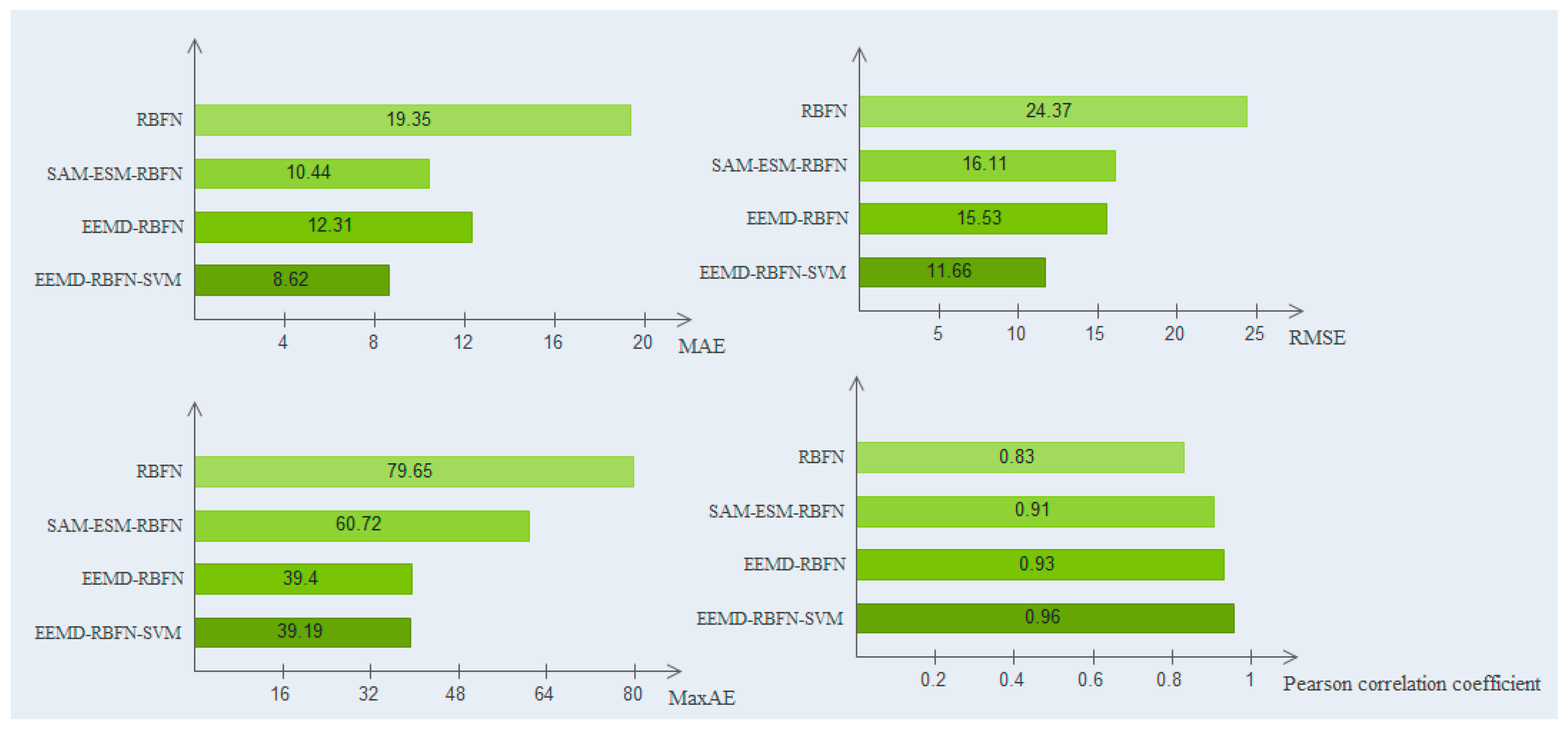
To assess the forecast capacity of the EEMD–RBFN–SVM model, four indices for error forecasting serve as the criteria to evaluate the forecasting performance. They are RMSE, MAE, MaxAE, and the Pearson correlation coefficient. Their effects are shown in
Table 1 and
Figure 10. For RMSE, MaxAE, and the Pearson correlation coefficient of the evaluation index, the prediction effect of the hybrid EEMD–RBFN–SVM model is the best, the EEMD–RBFN model is second, the SAM–ESM–RBFN mixture model is third, and the RBFN model is the worst. For the MAE index, the hybrid EEMD–RBFN–SVM model is still the best, the hybrid SAM–ESM–RBFN model is second, and the RBFN prediction effect is the worst. After a comparison of the above-mentioned models, it can be seen that all the indexes (RMSE, MAE, MaxAE, and the Pearson correlation coefficient) for the proposed model are lower. This indicates that the hybrid EEMD–RBFN–SVM model is an effective approach.
In addition, to fully illustrate the effectiveness of our proposed method, we used 75% of our data to calibrate our models and the remaining 25% of the data for a validation analysis of the “true forecasting” with these fitting parameters. The results were as follows:
MAE = 9.5291, RMSE = 12.8022, MaxAE = 44.9026,
Pearson correlation coefficient = 0.946.
All of those results indicate that the hybrid EEMD–RBFN–SVM model is the best approach of the tested methods.
5. Conclusions
Hydrological geological disasters have caused great suffering and serious economic losses for the civilian population, and it is necessary to propose an effective forecasting method to predict precipitation. A hybrid model based on EEMD, RBFN, and SVM (namely, the EEMD–RBFN–SVM model) is proposed in this study, and this model is applied to the precipitation data of the Qinghai Province Yushu Tibetan Autonomous Region. The results show that this hybrid model has a good prediction effect, can accurately predict precipitation data, and in a comparison, the hybrid model outperforms the RBFN network, the EEMD–RBFN model and the SAM–ESM–RBFN mixture model. Good prediction effects have been achieved in precipitation data forecasting thanks to these models.
This hybrid EEMD–RBFN–SVM model has the following advantages. Via the decomposition of the original sequence using EEMD, the nonstationary and nonlinear signal sequence is decomposed into a set of steady state and linear sequence, which enables us to fully use all the information in the sequence. RNFN is used to predict the decomposition of the sequence set because it has a better ability for nonlinear fitting than the general neural network and can approach any nonlinear function with any precision. This makes RBFN capable of predicting the decomposition sequence effectively. Finally, SVM is adopted to further optimize the prediction error of the sequence, so that the prediction accuracy can be further improved. This hybrid model fully considers various factors, from decomposition to prediction to error correction, and achieves a good prediction effect in hydrological data forecasting by making the best use of the information hidden in the sequence. Therefore, the proposed approach can improve the prediction accuracy effectively.
Accurate prediction of rainfall can provide a good reference for flood control, and our study allows us to better predict the precipitation. However, aspects remain that require further study. In this study, a cross validation was applied to determine the optimal hyper-parameters of SVM. There are other ways to optimize the parameters, such as the genetic algorithm (GA), particle swarm optimization (PSO) [
34], artificial bee colony (ABC), and harmony search (HS). In our future studies, we will consider optimizing the model using these methods. Even though there are still several shortcomings in our research, the model we proposed can solve the problem of precipitation forecasting to a certain extent and can therefore contribute to flood control.


