Characterization of a Flood Event through a Sediment Analysis: The Tescio River Case Study

Abstract

This paper presents the hydrological analysis and grain size characteristics of fluvial sediments in a river basin and their combination to characterize a flood event. The overall objective of the research is the development of a practical methodology based on experimental surveys to reconstruct the hydraulic history of ungauged river reaches on the basis of the modifications detected on the riverbed during the dry season. The grain size analysis of fluvial deposits usually requires great technical and economical efforts and traditional sieving based on physical sampling is not appropriate to adequately represent the spatial distribution of sediments in a wide area of a riverbed with a reasonable number of samples. The use of photographic sampling techniques, on the other hand, allows for the quick and effective determination of the grain size distribution, through the use of a digital camera and specific graphical algorithms in large river stretches. A photographic sampling is employed to characterize the riverbed in a 3 km ungauged reach of the Tescio River, a tributary of the Chiascio River, located in central Italy, representative of many rivers in the same geographical area. To this end, the particle size distribution is reconstructed through the analysis of digital pictures of the sediments taken on the riverbed in dry conditions. The sampling has been performed after a flood event of known duration, which allows for the identification of the removal of the armor in one section along the river reach under investigation. The volume and composition of the eroded sediments made it possible to calculate the average flow rate associated with the flood event which caused the erosion, by means of the sediment transport laws and the hydrological analysis of the river basin. A hydraulic analysis of the river stretch under investigation was employed to verify the validity of the proposed procedure.

1. Introduction

The grain size distribution over a riverbed significantly affects sediment transport and deposition and is therefore one of the most important factors influencing river hydraulics, hydrology and morphology [1,2,3,4,5,6]. At the same time, flood events have a major impact on the structure of watercourses, as they affect grain entrainment, transport and deposition, and a proper monitoring of the sediment size distribution may help to characterize the sequences of flood events in terms of duration and magnitude [7,8,9,10,11].

The estimation of the sediments’ size distribution can be performed using several different techniques, including direct measurement, dry and wet sieve analyses, laser measurements, and photographic sampling [6,7,8,12,13,14,15]. Each of these techniques has advantages and drawbacks and may be more or less suitable depending on the application. For example, traditional sieving usually requires a preliminary inspection, in order to identify the sampling sites where sediments are sufficiently stable and where the particle size range is not affected by local deposit factors (e.g., stagnation areas). Moreover, a sufficient sample must be taken, which is to say a sample with a weight at least 20 times heavier than the largest clast, extended deep down to the armoring [16]. Following this, the grain size analysis is performed and calibrated as a function of the mean dimensions of the collected clasts. While this approach may be extremely precise, it is also time-consuming and requires significant technical and economical resources. In addition, an accurate reconstruction of the grain size distribution over a wide area usually requires a high number of samples. Alternative solutions for investigating sediments in large areas are based on qualitative and quantitative on site analyses. Among the others, photographic sampling techniques have been developed in the last decade and demonstrated to be reliable and accurate [17,18,19,20,21,22,23,24,25,26,27].

The present paper discusses the development and application of a photographic sampling of fluvial sediments in gravel riverbeds, with the aim of also characterizing the flood history through sediment analysis. The proposed approach is both more cost and time effective with respect to traditional sampling techniques (e.g., sieving), while maintaining a sufficient degree of accuracy in measuring the particle size distribution for the kind of use envisaged.

The developed procedure is employed to characterize the particle size analysis in the riverbed of the Tescio River, a tributary of the Chiascio River, located in the center of Italy. In particular, the analysis has been performed on an ungauged river reach of 3 km subjected to a torrential regime, where traditional methods for the characterization of flash floods could not be employed. The photographic sampling was performed when the river was in dry conditions in nine sections, with the aim of identifying those characterized by removal of the armor (i.e., armoring). During the dry season, in fact, information can be obtained from the riverbed as the imprint of the significant flood phenomena occurs in the full season. The comparison of grain size distribution before and after the event allows for the estimation of the mean flow rate associated with the flood, by applying solid transport physical laws.

Such a photographic survey is particularly suitable for those riverbeds that remain dry for a long period, as those phenomena that produce changes in the granulometric equilibrium are easily and unequivocally detectable.

The present paper aims to propose an expeditious and practical indirect method to estimate the peak flow discharge of ungauged river channels with a torrential regime, on the basis of the analysis of erosion phenomena observed on the riverbed in dry conditions. In such conditions, flow data are often estimated with hydrological models that are affected by significant uncertainty.

The paper is organized as follows. Section 2 presents the case study and the river basin under investigation, together with the main results of the hydrological analysis. The photographic sampling technique and the estimation of the sediments’ size distribution are described in Section 3. Section 4 reports the analysis of the flood event through the proposed methodology, which allows for the estimation of the average water discharge, given the duration of the event. Moreover, a validation of the procedure is performed through a hydraulic analysis of the river stretch under investigation. Finally, conclusions drawn from the present research are presented.

2. Tescio River Basin Test Case

2.1. Site Description

The Tescio River Basin, chosen as the case study for the proposed methodology, is located in the center of Italy, in the Umbria Region (see Figure 1) [27], and has an extension of 67.9 km². The basin is part of the Tiber River Basin [28,29,30,31,32,33].

The main auction of the river starts from Monte dei Cani (871 m.a.s.l.) and the studied reach belongs to a stretch of about 20 km that terminates at the confluence with the Chiascio River, in Bastia Umbria, a small town at 206 m.a.s.l. In this stretch, there are three thermo-pluviometric stations and one hydrometric station located close to Ponte S. Vetturino in Assisi.

The morphology of the river basin is characterized by an elevation ranging from 206 m.a.s.l. (at the outfall to the Chiascio River) to 1290 m.a.s.l. (at the Monte Subasio). The lower basin (20%) and the upper basin (80%) have an average elevation of 300 m.a.s.l. and 600 m.a.s.l., respectively. The length of the Tescio River channel is 20.1 km with an average slope of 3%. The main characteristics of the basin are reported in

Table 1. Main characteristics of the Tescio River Basin. The quoted slopes refer to the basin.

Basin Dimensions
Area (km2)	67.9
Perimeter (km)	43.4
Length of the main stream (km)	20.1
Average elevation (m.a.s.l.)	562
Median elevation (m.a.s.l.)	550
Maximum elevation (m.a.s.l.)	1290
Minimum elevation (m.a.s.l.)	206
Basin Slopes
Maximum basin slope	5.39%
Average basin slope	3.00%
Alvard-Horton slope	31.61%

, while the hypsographic curve of the Tescio Basin is reported in Figure 2.

2.2. Hydrological Analysis

This section presents the main results of the hydrological analysis performed on the entire Tescio River Basin and some of the main sub-basins. First, the sections of interest along the Tescio River and its tributaries were set, and then a rainfall–runoff model was employed for the calculation of the design flow. The flow rate was calculated through an indirect method, which allows for the transformation of the rainfall that typically occurs in the water catchment area subtended by the section considered for the direct flow rate through the section itself. The necessity of such an indirect calculation is determined by the absence of measuring devices, such as hydrometers, while, on the other hand, several pluviometers are available on the dock.

The rainfall–flow rate transformation model used in this paper has been produced by joining two semi-analytical schematizations, in order to calculate the key hydrological processes in place: infiltration and surface runoff. More details on the hydrological analysis are reported in Appendix A.

Figure 3 depicts the sub-basins underpinned by the river sections under investigation and the schematization of the basin. The stretch of the river under investigation is located between the closure section of the sub-basin 1 and the total basin.

Table 2. Design flow rates (m³/s) for different return times (RT = 10, 50, 100, 200, and 500 years) for the total basin.

Years	RT = 10	RT = 50	RT = 100	RT = 200	RT = 500
Flow rates	12.52	88.04	116.86	148.46	191.98

reports the design flow rates of the total basin.

3. Grain Size Analysis

Figure 4 shows the location of the studied river reach, which has a length of about 3 km, and the nine cross sections, indicated as F1, F2, F3, F4, F5, F6, F7, F8, and F9, where the photos employed for the grain size analysis were taken. A picture of each of the nine investigated cross sections is shown in Figure 5.

The particle size analysis presented herewith is based on digital photos taken during the summer, when the studied river reach was in dry conditions. All of the pictures have been taken at a height of 120 cm from the ground, with a resolution of 1024 × 768 pixels. Each image features a metric element as a reference, in order to correctly reconstruct the scale of the photo.

Among the various techniques available to measure sediment grain distribution from digital photos [18,20,22,24,26], one based on the thresholding in grey scale and the segmentation of the resulting binary image was employed. The images analysis has been performed through the open source software ImageJ [34], following the procedure suggested in [24].

The employed reconstruction technique consists of the following fundamental steps.

• Image scale setting, to assign the metric parameters known for a portion of the image.
• Conversion into a grayscale image.
• Identification of the grains in the image. At this stage, the grayscale image is converted into a binary (black and white) one in which the grains are represented by white and black interstitial spaces. This phase consists of several sub-steps, as follows:

  • Application of a median filter to preserve edges while removing noise (as a default, 5 × 5 pixels was chosen).
  • Application of a “morphological filter”, a disk of radius set by the user (as a default, 15 pixels was chosen) to highlight the interstices that may be represented by dark areas without highlighting the grains. The morphological filter is a bottom hat filter. If the intensity values in a gray-level image are thought of as elevations, then a scene is composed of mountain tops (brightest points) and valley lows (darkest regions). A bottom hat filter preserves sharp bottoms and improves contrasts.
  • Conversion into a binary image by imposing a threshold of intensity. Two limit values were used, the first to identify any gaps and intergranular disorders, and the second to highlight the darker points that are certainly gaps. The two images obtained through the previous procedure are then combined in order to create a third in which the gaps of the first image coincide with those of the second.
• Separation of the grains. Often, at this stage of the process, the regions represented by the sediments are joined together. Therefore, the binary image is divided by applying the so-called “watershed transform”. An intensity parameter has been employed as a tolerance, to select regional minima and avoid over-segmentation, which occurs in an image where any small fluctuation in intensity represents a regional minima or maxima. By increasing the tolerance value, the number of segments is reduced, while, by decreasing it, more object splits are produced. This is the most delicate step of the entire procedure, given that, if the value of the intensity parameter is too small, an excessive segmentation of the grains is obtained, while too high a value may result in a lack of separation of the grains. To test the sensitivity of the procedure, values ranging between 0.2 and 2.0 were tested.
• Selection of sediments to be measured in the domain under study. The selected sediments include all the grains on the border of the selected domain. The output of this stage is a binary image containing only the sediments to be measured.
• Measurement of the grains (in pixels). For selected grains size, orientation, shape and surface were measured. At this stage, the information is expressed in pixels.
• Conversion of dimensions in metric units (mm). The measurements were converted to mm, using the scale set at the beginning of the process (Step 1).

The steps of the reconstruction technique are schematically represented in Figure 6.

3.1. Grain Size Distribution

The method used for the analysis of the grain size distribution is based on counting the number of grains of equal characteristics, as it was not possible to determine the weight of the mixture for a sampling based on photographic specimens. This can be done on an areal basis, measuring all the sediments (grains) within a specific area (areal sampling) or on a spot basis, considering only the grains lying on the nodes of a pre-defined grid (grid sampling) [35]. The two methods do not provide comparable results. In the areal sampling, in fact, all the grains have the same probability of being measured, while in the grid sampling, the probability of finding sediment of a given size in each grid point is proportional to its area. Both techniques have been adopted to the present test case and the granulometric curves produced with the described methods have been verified by comparison with in situ traditional sieving based on physical sampling. For the latter, we characterized the surface of the riverbed through a surface grid sampling (i.e., Wolman sample).

Figure 7 depicts the granulometric curves obtained with the grid-by-number and the area-by-number methods and reports the in-situ grain size measurements. Figure 8 depicts the d₅₀ (particle diameter at 50% in the cumulative distribution) and d₉₀ (particle diameter at 90% in the cumulative distribution) evolutions along the river reach through area-by-number, grid-by-number and in-situ measurements. It can be observed that the two methods give completely different results. However, both figures clearly show that the area-by-number method always underestimates the grain size with respect to in situ measurements. On the other hand, the agreement between the grid-by-number method and the in situ measurements is good in all analyzed images, except for picture F2 where the grain size is overestimated. Therefore, the grid-by-number method has been employed for the present study.

3.2. Results of the Sampling Procedure

The procedure described in the previous section made it possible to obtain a complete grain size characterization of the fluvial sediments synthesized by the grain size distribution curve (Figure 9) and by some other significant parameters, such as d₅₀ and d₉₀.

The main hydraulic factors that affect the grain size distribution along the river reach under investigation can be identified in three classes: anthropogenic, hydrodynamic and local.

The hydraulic works represent one of the most active anthropogenic factors affecting the grain size distribution, as for example in correspondence with bridge piers, the larger grains are usually concentrated in the central area of the riverbed upstream of the artifact, because of the regurgitation phenomenon and the consequent weakening of the current upstream. The effect of the hydraulic works on the grain size distribution can be seen in Figure 10, which shows the change in fluvial deposits along the Tescio River reach under investigation, as d₅₀ and d₉₀, highlighting the position of hydraulic transversal structures.

As for the hydrodynamic factors, the dominant parameter is the water depth, which, together with the size of the cross-section, is a function of the slope of the riverbed. Therefore, a direct correlation can be expected between the stress tensor in the riverbed and the water depth.

Among the local factors, in the present case study, it can be expected that the resurgence of the Chiascio River in its downstream section affects the riverbed grain distribution for about 100 m upstream from the confluence, where the flow velocity decreases, and is therefore not relevant in the present analysis.

The relationship between hydraulic parameters and grain size distribution is further discussed after the hydraulic simulation reported in Section 4.2.

4. Analysis of the Flood Event

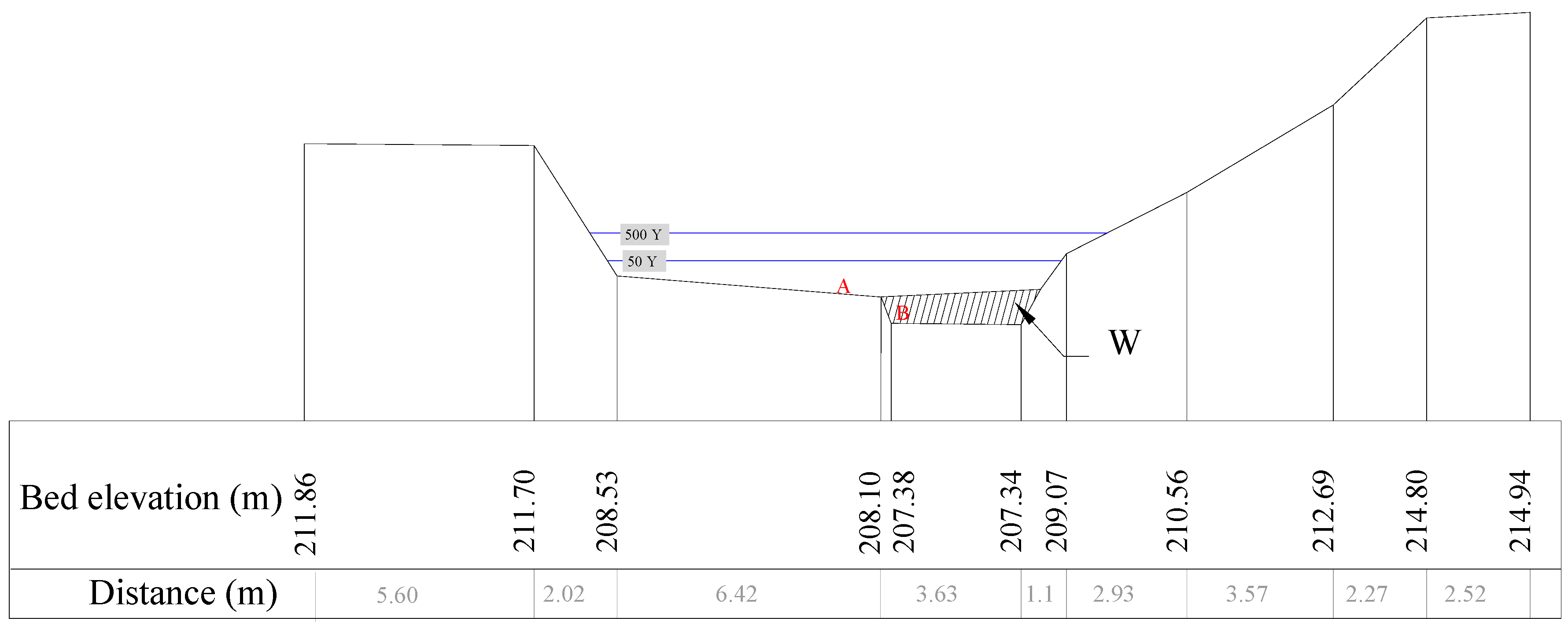
Thanks to a number of surveys made on site, it was possible to identify and determine the conditions of erosion and instability of the riverbed. Given the purpose of this work, it is worth noting the situation observed in the riverbed in a cross section located at about 1600 m (Section F7) from the confluence with the Chiascio River. There, an analysis of the sediments could be performed and the geometry of the section taken over when the riverbed was dry.

Through the monitoring done in the investigated river reach in dry conditions, the armor removal was only detected in this cross section. In fact, if the erosive event is sufficiently important, the state of the riverbed could be considered as a footprint, a snapshot that retains traces of the most significant floods recognizable with prolonged observation in time, and this is especially true for rivers with torrential water currents, such as the one analyzed in the present paper. It can be assumed that the observed erosion is a direct result of a flood wave propagation, as the hydraulics of the river reach under investigation are not affected by other relevant factors that may have contributed to the erosion of riverbed. Note that section F7 is representative of a river reach characterized by a regular cross-section, an almost constant slope, and a low sinuosity. Moreover, no significant obstacles (e.g., trees), bank erosions or anthropogenic changes are present. It can also be observed that the hydraulics of such a stretch is not affected by possible backwater caused by the confluence with the Chiascio River, which is about 1600 m downstream, or by river flow modifications caused by the human artifacts (i.e., the closest is the Tescio Bridge, which is about 500 m upstream).

No other significant erosive event was detected that could be attributed to a flood event in the river reach under investigation. This may be also related to the backwater of the Chiascio River, downstream, and to the presence of an armor layer with greater size grains, upstream, as detectable from Figure 8.

From the measurements made in the riverbed, it was possible to estimate the volume of the moved sediments and their granulometric composition. Figure 11 reports the grain size statistics as a cumulative curve showing the proportion of grains finer than a given size (i.e., granulometric curve).

The sediments were then classified following the Wentworth method [36]. The results, summarized in

Table 3. Size ranges of the sediments of section F7 given in the Wentworth scale.

Wentworth Class	% in Class
Boulder (>256 mm)	0.00
Cobble (64–256 mm)	55.52
Pebble (4–64 mm)	44.42
Granule (2–4 mm)	0.03
Sand (<2 mm)	0.02

, show that most of the sediments of the eroded volume are cobbles and pebbles.

Figure 12 shows the detailed geometry of the section under investigation and the eroded area. The survey of the armor removal during the dry season allowed for the estimation of a volume of the eroded sediments per unit length of about 3 m² for about 0.7 m of height. A view of the riverbed and two photographic samples at the cross section under investigation are reported in Figure 13.

Note that the thickness of the eroded material, measured in situ, also includes the sub-layer below the armoring with smaller particle size material, in the percentage represented by the granulometric curve, as shown in Figure 11.

4.1. Flood Event Characterization

The main objective of the present study is to calculate the average mass flow rate associated to a flood event, starting from the erosion caused by the flood event and observed in the river section. Such an assessment is performed through the adoption of sediment transport analytical formulations.

The solid transport relationships clearly show that the smaller the grain size, the greater the transport capacity of the flow. Therefore, in natural streams, small particles are transported downstream faster than large ones. Such an effect is mitigated by the mixing of the materials coming from upstream and by the action of larger grains that shelter the finer substrate grains from entrainment. The above phenomenon, usually called armoring, determines the particle size distribution over the riverbed with a coarse surface layer (i.e., armor layer) on the bed surface [37,38]. On the other hand, armor layers break-up under the action of important flood events [39,40] and an estimate of the moved material could allow for the characterizing the flood event itself.

The following model is that proposed Meyer-Peter et al. [41], obtained by interpreting the results of extensive experimental research conducted in the laboratory of outflowing currents in uniform flow conditions and, mainly, with monogranular materials. In particular, it can be assumed that the volumetric flow rate of the sediment transport per unit length, q_s, is a function of the water flow rate, the grain diameter, d; the solid material density, ρ_s; and the Shields parameter or criterion, ψ which measures the beginning of the motion of the sediment flow. This allows calculating q_s through the following relationship:

$$q_s=8{\left(\mathsf{\psi }-{\mathsf{\psi }}_{cr}\right)}^{1.5}\sqrt{g\frac{{\rho }_s-\rho }{\rho }}{d}^{3/2}$$

(1)

where g is the gravity acceleration, ψ is the Shields parameter on the bottom of the riverbed and ψ_cr is the critical Shield parameter calculated at the incipient motion flow conditions.

Given the flood duration, T, assessed in two hours, and the volume of the moved sediments per unit length, W_s, estimated in 3 m², the average value of q_s was calculated as follows:

$$q_s=\frac{W_s}{T}$$

(2a)

The above expression, however, assumes that the eroded material has a uniform grain size distribution, which is not true for real riverbeds. Therefore, it is necessary to employ a relationship that calculates the overall solid flow rate by weighting the flow rates, q_si, associated with the different grain diameters, d_i, as follows:

$$q_s=\frac{W_s}{T}=\frac{{\displaystyle \sum _i{p}_i{q}_{si}}}{100}$$

(2b)

where the weights, p_i, need to be calculated.

The evaluation of the incipient motion is performed by imposing the dynamic equilibrium between the forces acting on the grains invested by the flow [42] as follows:

$$\mathsf{\psi }=\frac{u_{*}^2}{g\frac{{\rho }_s-\rho }{\rho }d}=f_s\left(\frac{u_{*}d}{\upsilon }\right)$$

(3)

where $u_{*}$ is the friction velocity, calculated as:

$$u_{*}=\sqrt{\frac{{\tau }_0}{\rho }}$$

(4)

In Equation (4), τ₀ is the total bed critical shear stress on the wetted perimeter.

The function ψ is evaluated through the Shields diagram [43], which was experimentally derived and is typically used to identify the initiation of the sediment motion, by relating the dimensionless shear stress (also known as Shields stress) necessary to cause sediment movement with the grain shear Reynolds number, Re*, calculated as:

$$\mathrm{Re}*=\frac{u_{*}d}{\upsilon }$$

(5)

where ν is the kinematic viscosity of water.

The Shields diagram separates the motion area from the still one: the points that lie below the boundary curve identify the condition when the motion of the water is not sufficiently high to move the grains (ψ < ψ_cr), while the points that lie above the curve represent the sediment movement conditions.

The value of ψ_cr is here calculated as a function of the grain characteristic length in incipient motion conditions through the Brownlie fit of the Shields diagram [43]:

$${\mathsf{\psi }}_{cr}=0.22D_{*}^{-0.6}+0.06\text{exp}\left(-17.77D_{*}^{-0.6}\right)$$

(6)

where $D_{*}$ is a characteristic diameter defined as follows:

$$D_{*}=d{\left[g\frac{{\rho }_s-\rho }{\rho v^2}\right]}^{1/3}$$

(7)

As already discussed, natural waterways are characterized by a riverbed bottom with heterogeneous granulometry, which has a different behavior, in the evaluation of incipient motion of sediments particles with respect to a bed consisting of homogeneous material. The mobility of smaller grains is reduced by the sheltering effect of larger stones that in turn have their mobility increased by their greater exposure. The change in the Shields parameter with the size of the particles constituting the sediment, d_i, is controlled by the hiding function:

$$\frac{{\mathsf{\psi }}_{cr,d_i}}{{\mathsf{\psi }}_{cr,d_a}}={\left(\frac{d_a}{d_i}\right)}^b$$

(8)

here calculated through the empirical formulations proposed by Hayashi et al. [44]:

$$\frac{{\mathsf{\psi }}_{cr,d_i}}{{\mathsf{\psi }}_{cr,d_a}}={\left(\frac{d_a}{d_i}\right)}_{\text{ for }}\left(\frac{d_a}{d_i}\right)<1$$

(9)

$$\frac{{\mathsf{\psi }}_{cr,d_i}}{{\mathsf{\psi }}_{cr,d_a}}={{\left[\frac{\log \left(8\right)}{\log \left(\raisebox{1ex}{$8d_i$}\!\left/ \!\raisebox{-1ex}{$d_a$}\right.\right)}\right]}^2}_{\text{ for }}\left(\frac{d_a}{d_i}\right)>1$$

(10)

As proposed by Egiazaroff [45], d_a was calculated as the weighted average of the grain diameters:

$$d_a=\frac{1}{100}{\displaystyle \sum }_i{p}_i{d}_i$$

(11)

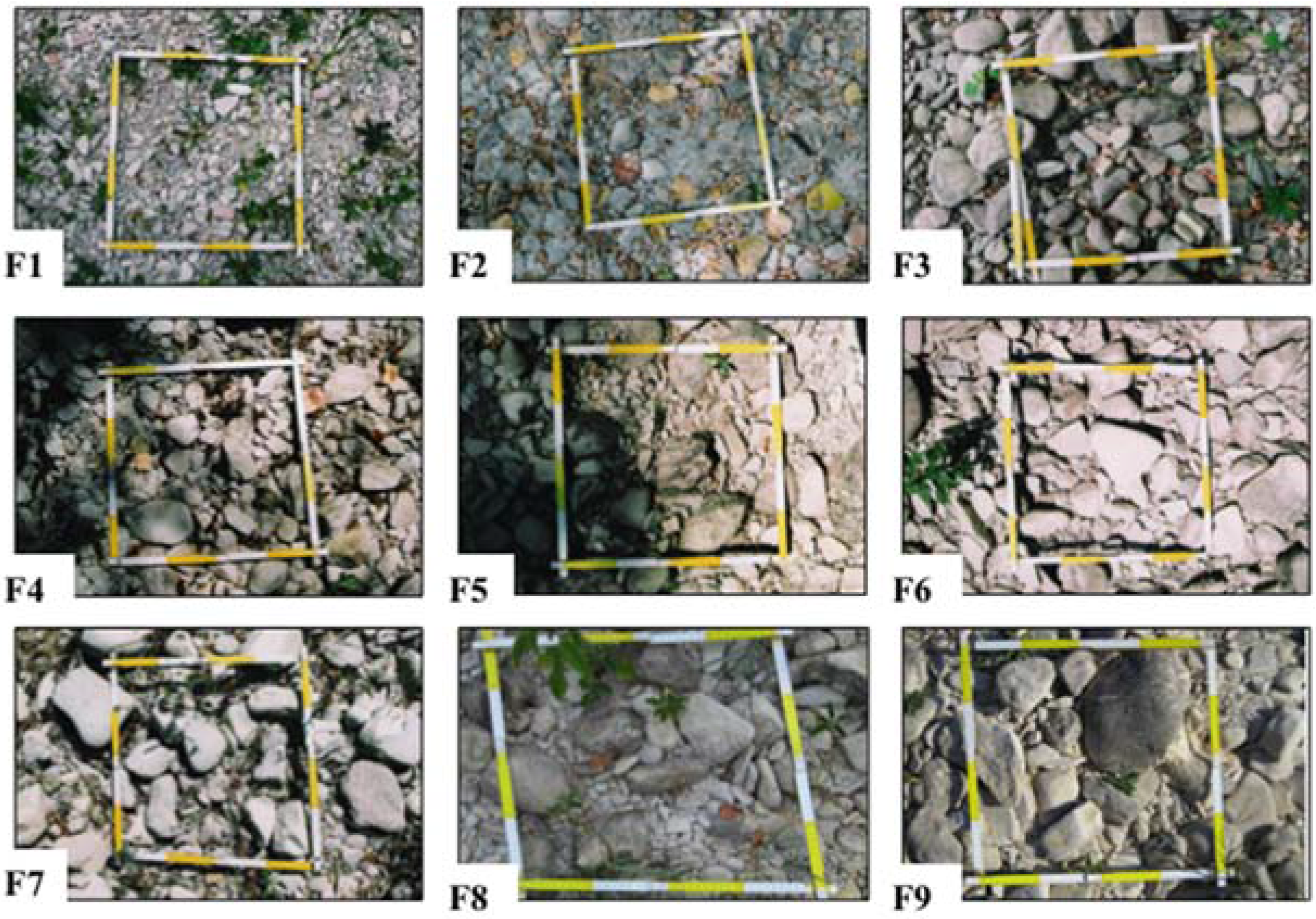
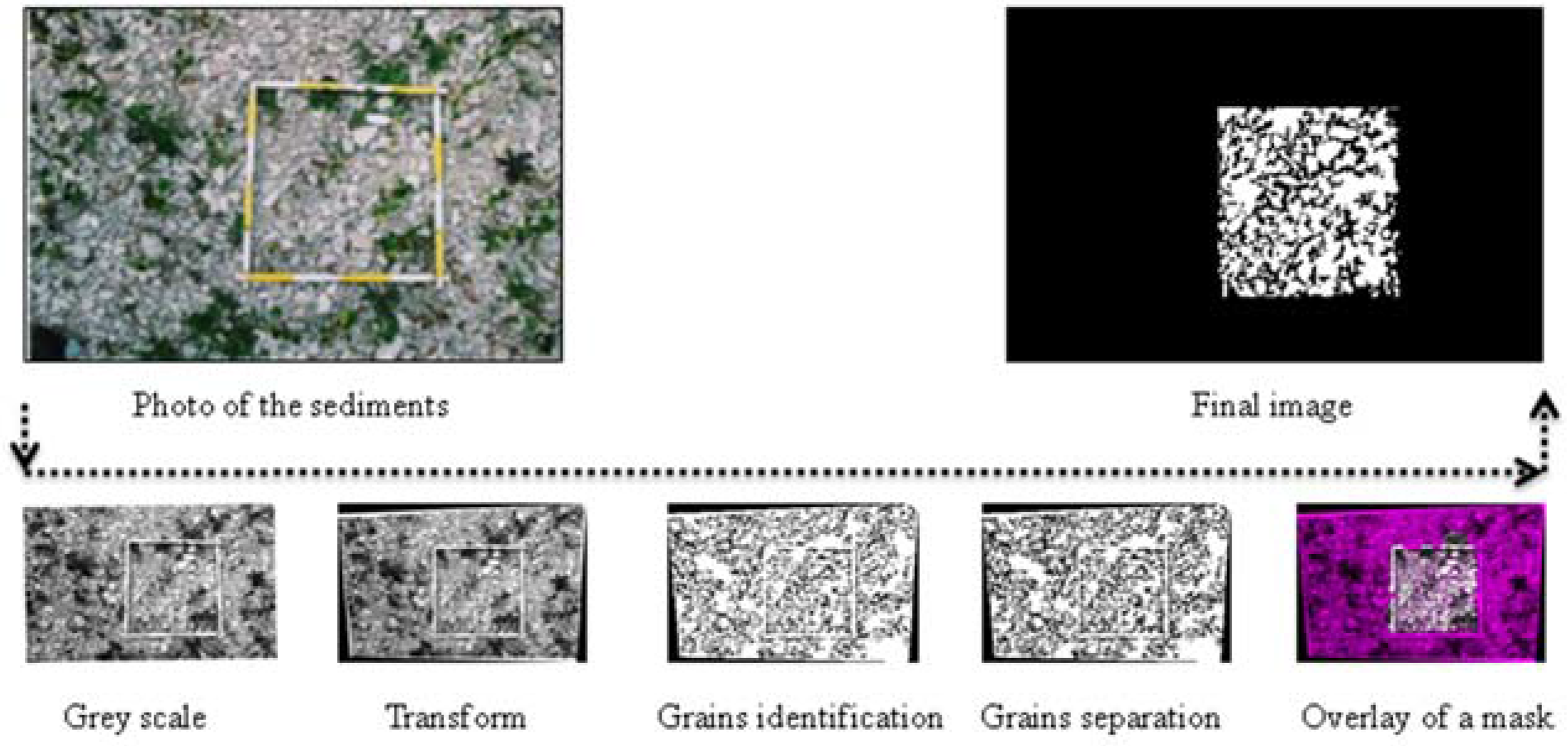
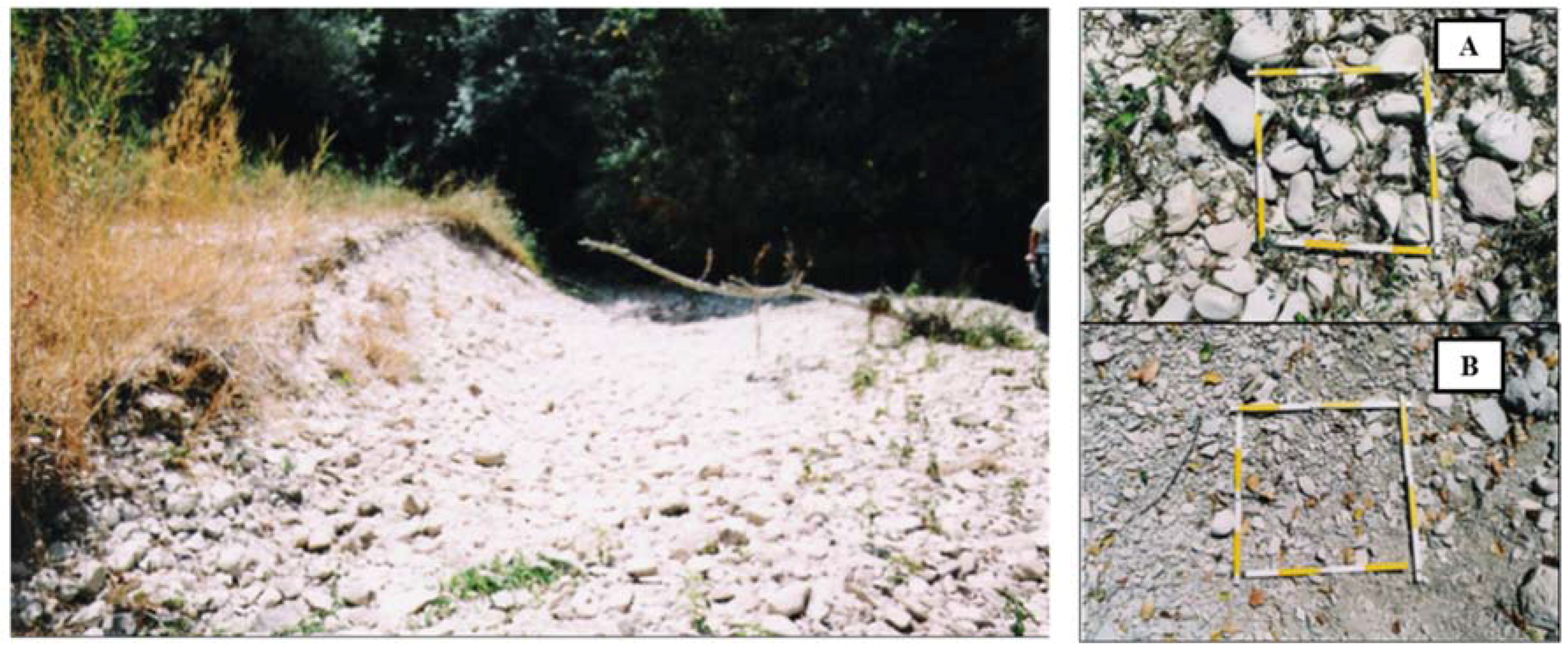
Then, the weights, p_i, were estimated by counting the number of grains of equal characteristics through the areal-based procedure previously described.

Table 4. Particle size distribution of the sediment eroded by the flood.

Sieve Size (mm)	Area of Size Class (mm2)	Percentage in Class (%)	Cumulative Percentage (%)
1.41	0.00	0.00	0.00
2.00	82.56	0.02	0.02
2.83	38.85	0.01	0.04
4.00	60.71	0.02	0.05
5.66	444.39	0.13	0.19
8.00	1189.88	0.35	0.54
11.31	2105.37	0.62	1.16
16.00	6046.56	1.79	2.96
22.63	11,986.27	3.56	6.51
32.00	26,709.27	7.93	14.44
45.25	38,486.70	11.42	25.86
64.00	62,743.36	18.62	44.48
90.51	58,365.07	17.32	61.80
128.00	97,483.14	28.93	90.72
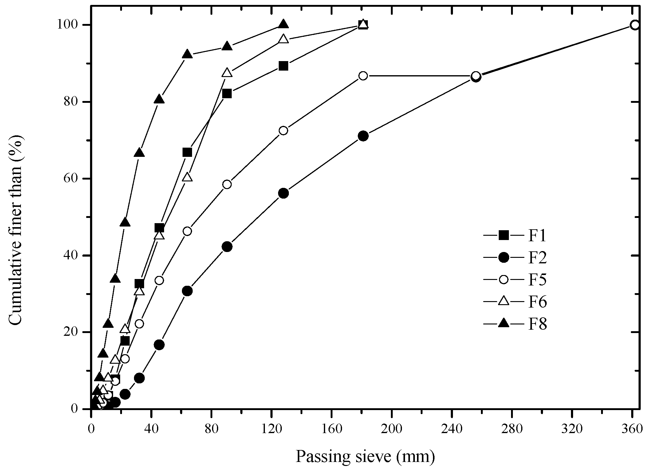
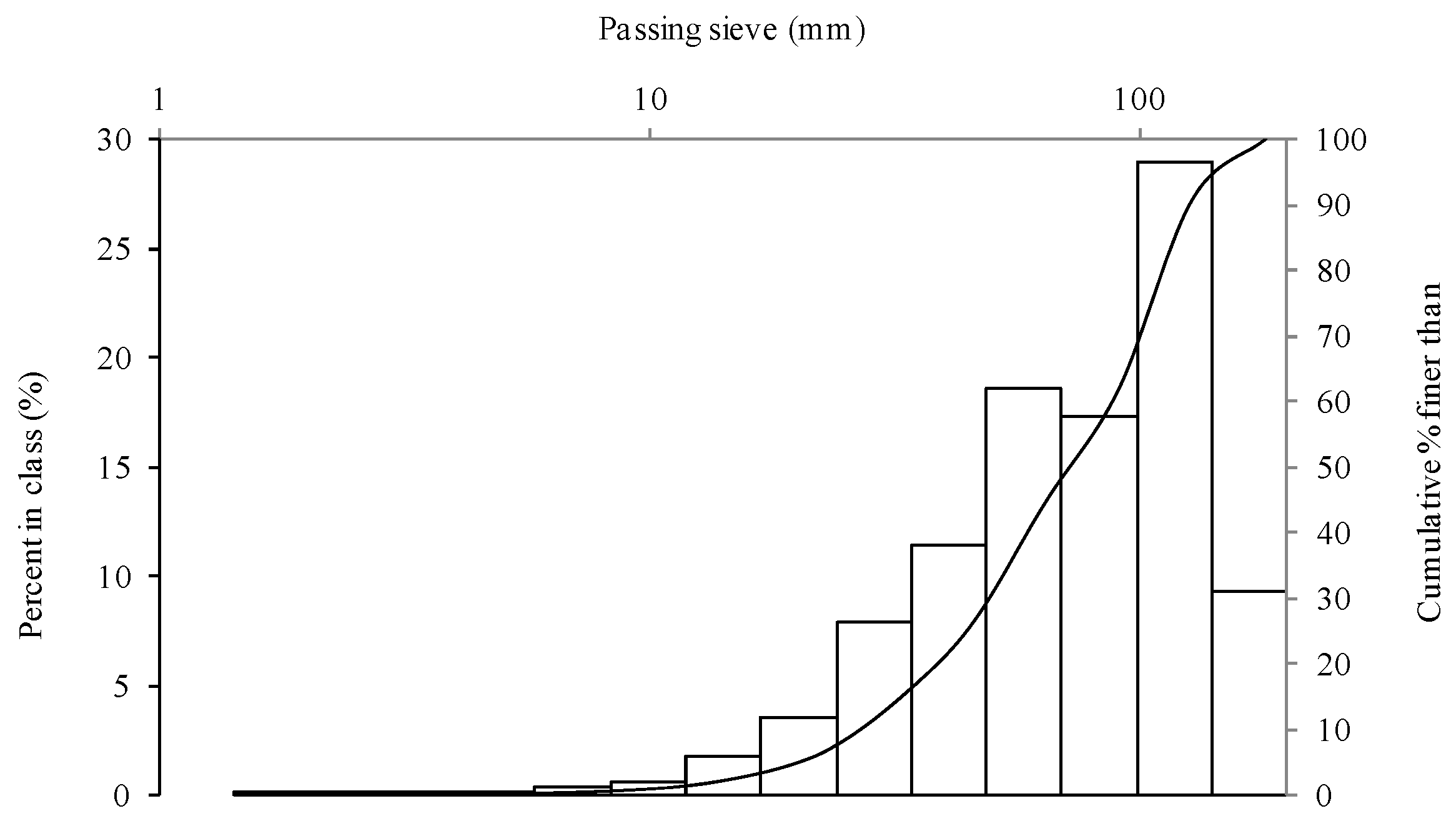
181.02	31,272.12	9.28	100.00

reports the measured grain distribution, from which d_a results as equal to 90.33 mm.

The sediment transport value relative to the diameters d_i can be calculated using Equation (1).

Given the structure of the river reach under investigation, the piezometric surface, j, can be assumed to be equal to the slope of the bottom of the riverbed, i. Therefore, ψ_i can be derived from Equation (12) as follows:

$${\mathsf{\psi }}_i=\frac{{\tau }_0}{g\left({\rho }_s-\rho \right)d_i}=\frac{\gamma Ri}{g\left({\rho }_s-\rho \right)d_i}$$

(12)

In which γ is the specific weight of water and R is the hydraulic radius of the river section. By estimating ψ_i through the Shield’s diagram, it is possible to calculate R = 0.862 m and τ₀ = 73.53 Pa from Equation (12).

Following this, we applied the Chézy’s formula, which describes the mean flow velocity of steady-state turbulent open channel flows, to calculate the flow discharge, Q, by assuming a Manning’s roughness coefficient equal to 0.04 s/m^1/3. It results that the flow rate that caused the erosion during the flood event of known duration is about 22 m³/s.

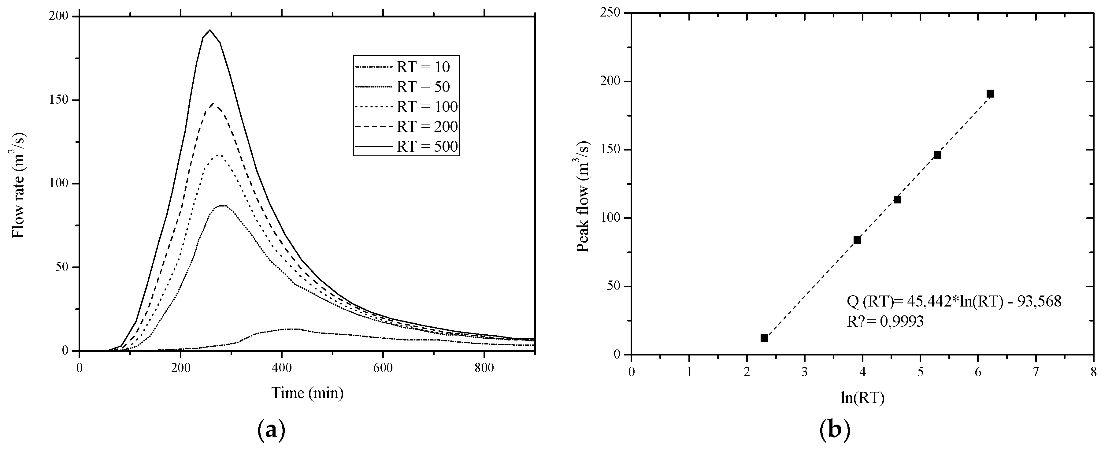
By linearly interpolating the hydrographs obtained through the hydrological analysis, the hydrographs in the river section under investigation for different return periods were obtained, as depicted in Figure 14a. Figure 14b shows the peak flow rates as a function of the return period and the corresponding linear regression, which, in turn, allows for a calculation of a return period of 13 years associated with a flood discharge of 22 m³/s.

4.2. Hydraulic Analysis and Procedure Validation

A validation of the above procedure is here performed through the hydraulic numerical simulation of the river basin under investigation. In particular, the Hec-Ras software was employed to calculate the water depth and the flood areas at different return periods (i.e., 50, 100, 200 and 500 years). The employed numerical modeling is based on a one-dimensional steady flow. Energy losses were calculated through Manning’s equation. Consistent with the approximation of the proposed procedure, the hydraulic analysis was carried out at a fixed riverbed, based on the pre-flood geometry. In the river sections where the current varies rapidly (e.g., bridges, hydraulic jumps, and weirs), the model solves the momentum equation.

The other input data necessary for the hydraulic simulations include geometric data, such as cross section profiles and the slope of the river reach, roughness coefficients, and inlet and outlet boundary conditions (i.e., flow discharges). In particular, the hydraulic simulation was performed in a 13 km long river reach, in order to avoid effects of the boundary conditions, and 72 cross sections were surveyed. Moreover, the water discharges at the different RTs are directly drawn from the results of the hydrologic analysis reported in Section 2.

The results of the hydraulic simulations for the cross section under investigation are reported in

Table 5. Summary of the hydraulic analysis results for different return periods (10, 50, 100, 200, and 500 years). Q is design flow rate, h₁ is the geodetic height, h is the water height, h_c is the critical water height, v is the mean velocity, A is the wetted section, Fr is the Froude number, and τ₀ is the total bed critical shear stress on the wetted perimeter.

RT (Years)	Q (m3/s)	h1 (m)	h (m)	hc (m)	v (m/s)	A (m2)	Fr	τ0 (Pa)
50	88.04	207.12	208.90	208.74	2.71	32.51	0.80	226.52
100	116.86	207.12	209.11	208.95	3.05	38.33	0.84	257.482
200	148.46	207.12	209.31	209.17	3.37	44.05	0.87	279.09
500	192.00	207.12	209.56	209.44	3.75	51.20	0.90	304.99

, where the water discharges at different RTs are also associated to different critical shear stresses.

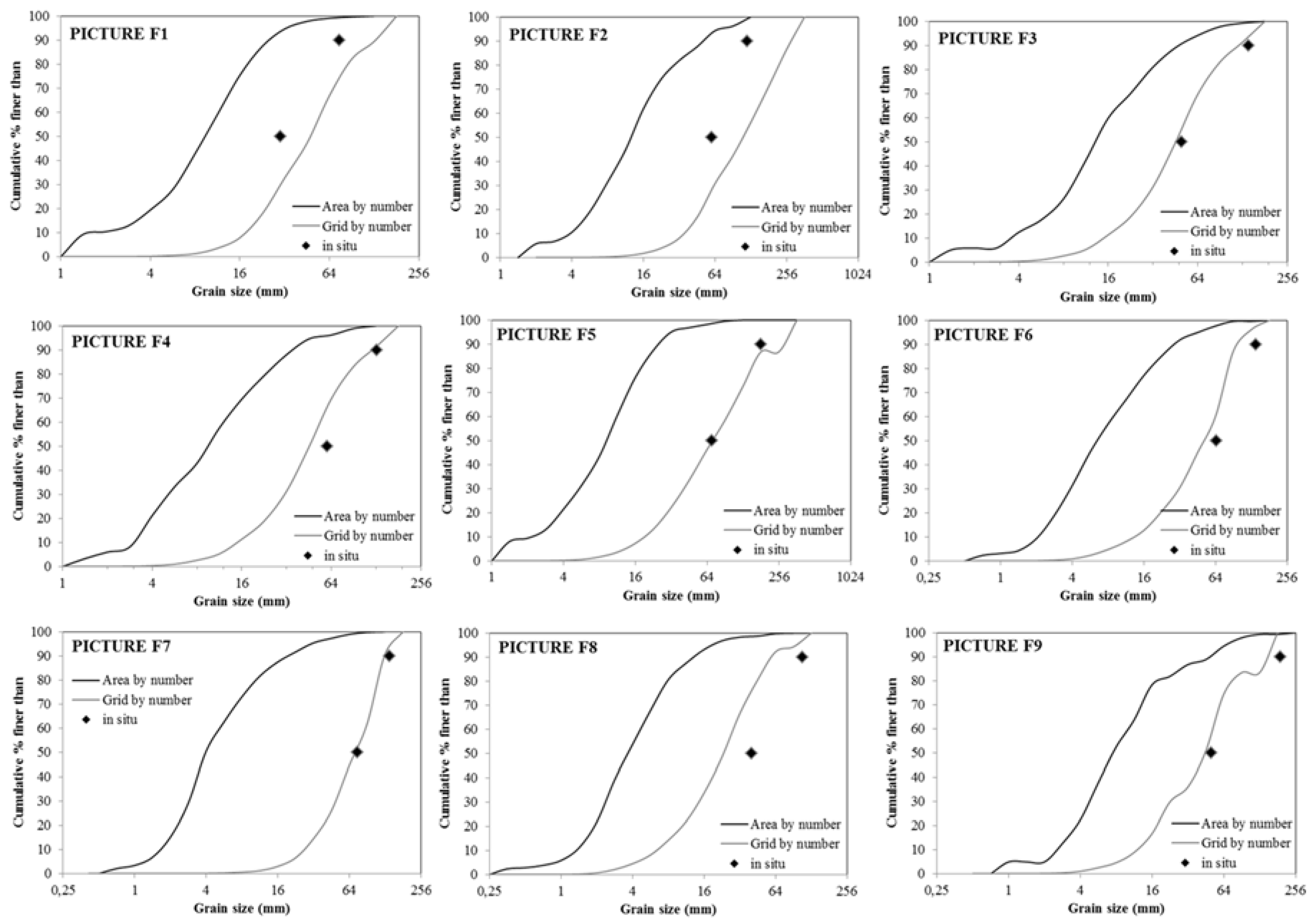
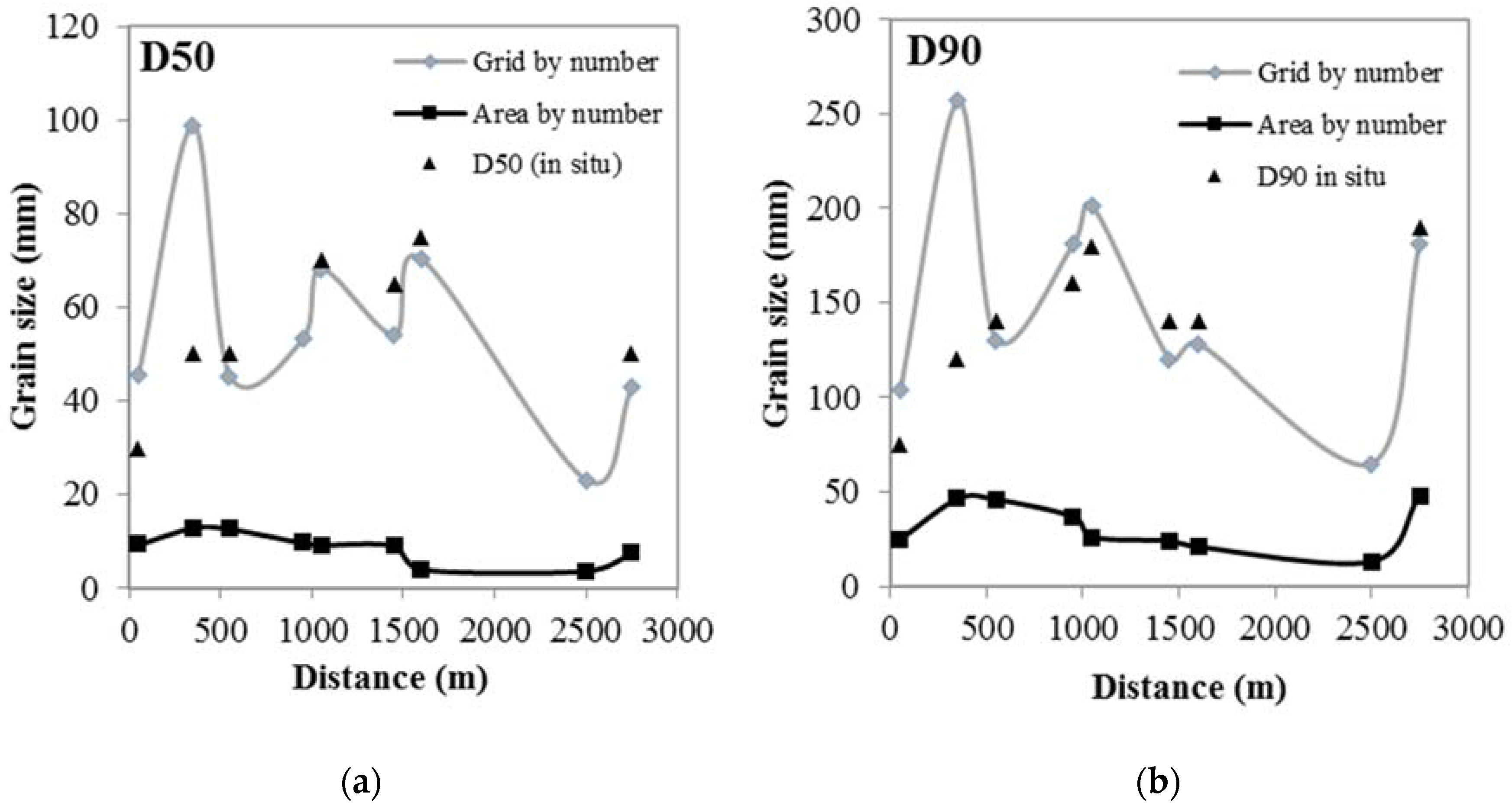
The hydraulic effects on the grain size distribution are evidenced by the data summarized in

Table 6. Evolution of channel characteristics and hydraulic parameters along the river reach under investigation.

Distance (m)	τ0 TR 50 (N/m2)	Velocity (m/s)	Wetted Area (m2)	d50 (GbN) (mm)	d90 (GbN) (mm)
50	39.45	1.7	61.24	45.39	104.03
350	142.64	2.53	42.63	98.9	256.8
550	121.03	2.38	49.15	45.33	130
950	100.54	1.71	51.63	42.04	181
1050	141.20	1.77	67.1	54.7	201
1450	107.26	0.81	109.13	68.25	120
1600	226.51	2.95	29.89	70.36	128.3
2500	130.56	2.49	35.36	23.04	65
2750	96.30	1.35	65.11	42.87	181

, which reports the d₅₀ and d₉₀ values of the nine cross sections under investigation together with the critical shear stress, the flow velocity, and the wetted area. In particular, it can be observed that, as a general trend, d₅₀ and d₉₀ increase with the shear stress and decrease with the wetted area. However, it should be noted that such a relationship is more complex, as differences in grain size with the same shear stress may also be observed locally, as for example in section F2, which has the same τ as section F5, with a comparable d₅₀ but almost double the d₉₀.

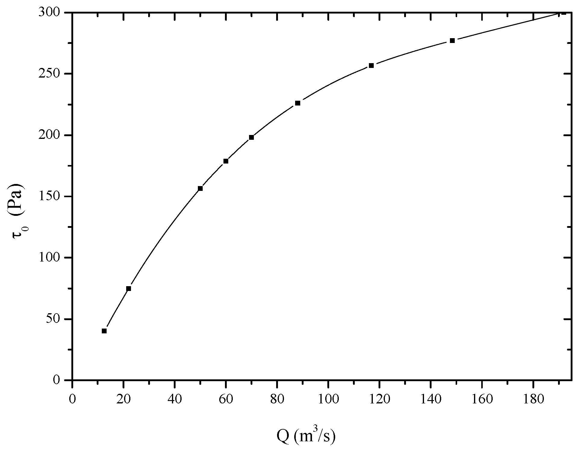
Through the hydraulic simulations, the relationship between Q and τ₀ in section F7 was constructed, as depicted in Figure 15. From this relationship, a critical shear stress of 74.79 Pa associated to the flow discharge of the flood event equal to 22 m³/s was calculated. Such a value is in excellent agreement with that calculated through Equation (12) (τ₀ = 73.53 Pa).

5. Conclusions

The present paper presents the application of a photographic sampling method to the sediments forming the bed of a 3 km reach of the Tescio River, located in the center of Italy, characterized by a length of 20.1 km and an average slope of 3%.

First, a hydrological analysis of the basin was performed, through which the design hyetographs were determined, the basin in plane and channel elements was schematized, the rainfall–runoff model for the calculation of the design flow was calibrated, and the design hydrographs for the basin and sub-basins under investigation related to return periods of 10, 50, 100, 200 and 500 years were calculated.

The grain size distribution analysis is based on digital photos taken when the river was in dry conditions and was performed through the thresholding in grey scale and the segmentation of the resulting binary image. The image analysis was performed using open source software. The procedure has provided good results in determining the particles size distribution.

The performed calculations were then used to estimate the water flow rate of a flood from an erosive event, starting from the erosion caused by the flood event and observed in a river cross section. The whole river reach has been inspected in dry conditions and the only significant armor removal was observed in one cross section, where the erosive event took away a sufficiently large volume of material to be measured with acceptable accuracy.

Through the adoption of sediment transport analytical formulations, it was possible to estimate an average mass flow rate associated to the flood event of 22 m³/s, corresponding to a return period of about 13 years. Finally, a one-dimensional hydraulic analysis of the river reach was performed. The above procedure was validated by calculating the total bed critical shear stress on the wetted perimeter in the cross section under investigation and comparing it with that calculated through the sediment analysis.

It should be noted that riverbed erosion is a complex phenomenon that cannot be completely characterized by the proposed analytical model based on empirical relationships. Therefore, the present procedure should be employed with the consideration in mind that local erosion might also be generated by other causes, such as local hydraulic effects or regressive erosion. In the present work, it is assumed that the observed erosion was attributable exclusively to the transit of a flood. The employed cross section is, in fact, representative of a stretch of the river with an even cross section, an almost constant slope, and low sinuosity. Moreover, there are no obstacles (e.g., trees), bank erosions or any other anthropogenic changes. It can also be observed that the flow in this river reach cannot be affected by possible backwater caused by the confluence with the Chiascio River, which is about 1600 m downstream, or by river flow modifications caused by human artifacts, which are sufficiently far upstream and downstream.

It is worth noting that the particularity of the present work is a methodology for the analysis of ungauged river basins with torrential river regime. While the proposed methodology is certainly affected by uncertainties, this paper demonstrates that it could be a valuable support to the hydraulic modeling of ungauged river reaches, where monitoring through traditional hydrological instruments is not economically viable. The proposed procedure may have other possible practical applications in ungauged river reaches. Such a method, in fact, might also integrate other observations, easily available in situ, to estimate the severity of a flood event, such as flood markers and modification of the riparian vegetation along the river channel. This information, which can be quantitatively gathered by experienced inspectors working on the ground for the control and maintenance of river channels, together with possible erosions of the riverbed, may also allow an indirect validation of rainfall–runoff models.

As a future development, the authors are working on the development of more sophisticated erosion and sediment-transport models.

References

1. Folk, R.L.; Ward, W.C. Brazos River bar: A study in the significance of grain size parameters. J. Sediment. Res. 1957, 27, 3–26. [Google Scholar] [CrossRef]
2. Folk, R.L. A review of grain-size parameters. Sedimentology 1966, 6, 73–93. [Google Scholar] [CrossRef]
3. Friedman, G.M. Differences in size distributions of populations of particles among sands of various origins. Sedimentology 1979, 26, 3–32. [Google Scholar] [CrossRef]
4. Bui, E.N.; Mazullo, J.; Wilding, L.P. Using quartz grain size and shape analysis to distinguish between aeolian and fluvial deposits in the Dallol Bosso of Niger (West Africa). Earth Surf. Process. Landf. 1990, 14, 157–166. [Google Scholar] [CrossRef]
5. Smart, G.; Aberle, J.; Duncan, M.; Walsh, J. Measurement and analysis of alluvial bed roughness. J. Hydraul. Res. 2004, 42, 227–237. [Google Scholar] [CrossRef]
6. Lopez, O.M.; Jadoon, K.Z.; Missimer, T.M. Method of relating grain size distribution to hydraulic conductivity in dune sands to assist in assessing managed aquifer recharge projects: Wadi Khulays dune field, western Saudi Arabia. Water 2015, 7, 6411–6426. [Google Scholar] [CrossRef]
7. Wolman, M.G. A method of sampling coarse river-bed material. EOS Trans. Am. Geophys. Union 1954, 35, 951–956. [Google Scholar] [CrossRef]
8. Dinehart, R.L. Evolution of coarse gravel bed forms: Field measurements at flood stage. Water Resour. Res. 1992, 28, 2667–2689. [Google Scholar] [CrossRef]
9. Bridge, J.S. Rivers and Floodplains: Forms, Processes, and Sedimentary Record; John Wiley and Sons: Hoboken, NJ, USA, 2009. [Google Scholar]
10. Habersack, H.; Piegay, H.; Rinaldi, M. Gravel Bed Rivers 6: From Process Understanding to River Restoration; Elsevier: Amsterdam, The Netherlands, 2011; Volume 11. [Google Scholar]
11. Gurnell, A.M.; Bertoldi, W.; Corenblit, D. Changing river channels: The roles of hydrological processes, plants and pioneer fluvial landforms in humid temperate, mixed load, gravel bed rivers. Earth Sci. Rev. 2012, 111, 129–141. [Google Scholar] [CrossRef]
12. Diplas, P.; Sutherland, A.J. Sampling techniques for gravel sized sediments. J. Hydraul. Eng. 1988, 114, 484–501. [Google Scholar] [CrossRef]
13. Blott, S.J.; Pye, K. Gradistat: A grain size distribution and statistics package for the analysis of unconsolidated sediments. Earth Surf. Process. Landf. 2001, 26, 1237–1248. [Google Scholar] [CrossRef]
14. Aberle, J.; Smart, G.M. The influence of roughness structure on flow resistance on steep slopes. J. Hydraul. Res. 2003, 41, 259–269. [Google Scholar] [CrossRef]
15. Rüther, N.; Huber, S.; Spiller, S.; Aberle, J. Verifying a photogrammetric method to quantify grain size distribution of developed armor layers. In Proceedings of the 35th IAHR Congress, Chengdu, China, 8–13 September 2013.
16. Roberts, R.G.; Church, M. The sediment budget in severely disturbed watersheds, Queen Charlotte Ranges, British Columbia. Can. J. For. Res. 1986, 16, 1092–1106. [Google Scholar] [CrossRef]
17. Adams, J. Gravel size analysis from photographs. J. Hydraul. Div. 1979, 104, 1247–1255. [Google Scholar]
18. Ibbeken, H.; Schleyer, R. Photo-sieving: A method for grain-size analysis of coarse-grained, unconsolidated bedding surfaces. Earth Surf. Process. Landf. 1986, 11, 59–77. [Google Scholar] [CrossRef]
19. Butler, J.B.; Lane, S.N.; Chandler, J.H. Automatic extraction of grain-size data from gravel surfaces using digital image processing. Am. Soc. Civ. Eng. J. Hydraul. Div. 2001, 39, 519–529. [Google Scholar]
20. Lane, S.N. The measurement of gravel-bed river morphology. In Gravel-Bed Rivers V; Mosley, M.P., Ed.; Caxton Press: Christchurch, New Zealand, 2001; pp. 291–338. [Google Scholar]
21. Sime, L.C.; Ferguson, R.I. Gravel-bed river grain size information by automated image analysis. J. Sediment. Res. 2003, 73, 630–636. [Google Scholar] [CrossRef]
22. Graham, D.J.; Rice, S.P.; Reid, I. A transferable method for the automated grain sizing of river gravels. Water Resour. Res. 2005, 41, 226–244. [Google Scholar] [CrossRef]
23. Graham, D.J.; Rollet, A.J.; Piégay, H.; Rice, S.P. Maximizing the accuracy of image-based surface sediment sampling techniques. Water Resour. Res. 2010, 46, 71–73. [Google Scholar] [CrossRef]
24. Strom, K.B.; Kuhns, R.D.; Lucas, H.J. Comparison of automated image-based grain sizing to standard pebble-count methods. J. Hydraul. Eng. 2010, 136, 461–473. [Google Scholar] [CrossRef]
25. Guerrero, M.; Rüther, N.; Szupiany, R.N. Laboratory validation of acoustic Doppler current profiler (ADCP) techniques for suspended sediment investigations. Flow Meas. Instrum. 2012, 23, 40–48. [Google Scholar] [CrossRef]
26. Cislaghi, A.; Chiaradia, E.A.; Bischetti, G.B. A comparison between different methods for determining grain distribution in coarse channel beds. Int. J. Sediment Res. 2016. [Google Scholar] [CrossRef]
27. Guerrero, M.; Rüther, N.; Szupiany, R.; Haun, S.; Baranya, S.; Latosinski, F. The Acoustic Properties of Suspended Sediment in Large Rivers: Consequences on ADCP Methods Applicability. Water 2016, 8, 13. [Google Scholar] [CrossRef]
28. Manciola, P.; Di Francesco, S.; Biscarini, C. Flood Protection and Risk Management: The Case of Tescio River Basin. In Proceedings of the Role of Hydrology in Water Resources Management, Capri, Italy, 13–16 October 2008.
29. Manciola, P.; Casadei, S. Criteria for the evaluation of the rate of water use in a river basin. Int. Assoc. Hydrol. Sci. Publ. 1995, 231, 169–179. [Google Scholar]
30. Ubertini, L.; Manciola, P.; Casadei, S. Evaluation of the minimum instream flow of the Tiber River Basin. Environ. Monit. Assess. 1996, 41, 125–136. [Google Scholar] [CrossRef] [PubMed]
31. Pierleoni, A.; Bellezza, M.; Casadei, S.; Manciola, P. Multipurpose water use in a system of reservoirs. IAHS Publ. Ser. Proc. Rep. 2007, 315, 107–116. [Google Scholar]
32. Nardi, F.; Annis, A.; Biscarini, C. On the impact of urbanization on flood hydrology of small ungauged basins: The case study of the Tiber river tributary network within the city of Rome. J. Flood Risk Manag. 2015. [Google Scholar] [CrossRef]
33. Nardi, F.; Biscarini, C.; Di Francesco, S.; Manciola, P.; Ubertini, L. Comparing A Large-Scale Dem-Based Floodplain Delineation Algorithm With Standard Flood Maps: The Tiber River Basin Case Study. Irrig. Drain. 2013, 62, 11–19. [Google Scholar] [CrossRef]
34. Ferreira, T.; Rasband, W. ImageJ User Guide, IJ 1.46r. Available online: https://imagej.nih.gov/ij/docs/guide/ (accessed on 19 July 2016).
35. Graham, D.J.; Ian, R.; Stephen, P.R. Automated sizing of coarse-grained sediments: Image-processing procedures. Math. Geol. 2005, 37, 1–28. [Google Scholar] [CrossRef]
36. Wentworth, C.K. A Scale of Grade and Class Terms for Clastic Sediments. J. Geol. 1922, 30, 377–392. [Google Scholar] [CrossRef]
37. Parker, G.; Sutherland, A.J. Fluvial armor. ASCE J. Hydraul. Eng. 1990, 28, 529–544. [Google Scholar] [CrossRef]
38. Jain, S.C. Armor or pavement. ASCE J. Hydraul. Eng. 1990, 116, 436–440. [Google Scholar] [CrossRef]
39. Parker, G.; Klingeman, P. On why gravel bed streams are paved. Water Resour. Res. 1982, 18, 1409–1423. [Google Scholar] [CrossRef]
40. Vericat, D.; Batalla, R.J.; Garcia, C. Breakup and reestablishment of the armour layer in a large gravel-bed river below dams: The lower Ebro. Geomorphology 2006, 76, 122–136. [Google Scholar] [CrossRef]
41. Meyer-Peter, E.; Müller, R. Formulas for bed-load transport. In Proceedings of the 2nd Meeting, IAHR, Stockholm, Sweden, 7–9 June 1948; pp. 39–64.
42. Shields, A. Anwendung der Aenlichkeitsmechanik und der Turbolenzforschung auf die Geschiebebewegung. In Doktor-Ingenieurs Dissertation; Technischen Hochschule: Berlin, Germany, 1936. [Google Scholar]
43. Brownlie, W.R. Prediction of Flow Depth and Sediment Discharge in Open Channels; California Institute of Technology: Pasadena, CA, USA, 1981. [Google Scholar]
44. Tatsuzawa, H.; Hayashi, H.; Hasegawa, K. Role of heterogeneous property of bed materials in the formation of step-pool systems in mountain streams. J. Hydrosci. Hydraul. Eng. 1999, 17, 37–45. [Google Scholar] [CrossRef]
45. Egiazaroff, I.V. Calculation of nonuniform sediment concentrations. J. Hydraul. Div. 1965, 91, 225–246. [Google Scholar]
46. Corradini, C.; Melone, F.; Moramarco, T.; Morbidelli, R. Basin representation and direct runoff hydrograph for different basin sizes. In Modeling and Simulation; Hamza, M.H., Ed.; IASTED ACTA Press: Anaheim, CA, USA, 1996; pp. 422–425. [Google Scholar]
47. Govindaraju, R.S.; Morbidelli, R.; Corradini, C. Use of similarity profiles for computing surface runoff over small watersheds. J. Hydrol. Eng. 1999, 4, 100–107. [Google Scholar] [CrossRef]
48. Corradini, C.; Govindaraju, R.S.; Morbidelli, R. Simplified modelling of areal average infiltration at the hillslope scale. Hydrol. Process. 2002, 16, 1757–1770. [Google Scholar] [CrossRef]
49. Grimaldi, S.; Serinaldi, F. Design hyetograph analysis with 3-copula function. Hydrol. Sci. J. 2006, 51, 223–238. [Google Scholar] [CrossRef]
50. Gräler, B.; van den Berg, M.; Vandenberghe, S.; Petroselli, A.; Grimaldi, S.; De Baets, B.; Verhoest, N. Multivariate return periods in hydrology: A critical and practical review focusing on synthetic design hydrograph estimation. Hydrol. Earth Syst. Sci. 2013, 17, 1281–1296. [Google Scholar] [CrossRef] [Green Version]
Figure 1. Map of the geographical area where the river under investigation is located.
Water 08 00308 g001
Figure 2. Hypsographic curve of Tescio River Basin.
Water 08 00308 g002
Figure 3. Sub-basins underpinned by the river sections under investigation.
Water 08 00308 g003
Figure 4. Map of the river reach under investigation. The section used to characterize the flood event is F7, located 1500 m upstream of the confluence with the Chiascio River. The surveyed cross sections are indicated in red and the surveyed and analyzed cross sections in blue.
Water 08 00308 g004
Figure 5. Sampling photos of the bottom channel of the sections under investigation.
Water 08 00308 g005
Figure 6. Schematic representation of the proposed reconstruction technique from the photo to the grain size distribution.
Water 08 00308 g006
Figure 7. Comparison of area- and grid-by-number granulometric curves for nine cross section of the river reach under investigation, named F1, F2, F3, F4, F5, F6, F7, F8, and F9. In situ measurements are also reported for comparison.
Water 08 00308 g007
Figure 8. Comparison of d50 (a) and d90 (b) estimation performed through area-by-number, grid-by-number and in-situ measurements. Distance is measured along the river channel starting from the Chiascio River confluence.
Water 08 00308 g008
Figure 9. Grain distribution along the riverbed at five selected sections (F1, F2, F5, F6, and F8).
Water 08 00308 g009
Figure 10. Change in fluvial deposits along the Tescio River reach under investigation as d50 and d90. The position of hydraulic transversal structures is also indicated.
Water 08 00308 g010
Figure 11. Cumulative grain size distribution of the handled volume in section F7.
Water 08 00308 g011
Figure 12. Tescio River cross section under investigation (i.e., F7) with the main dimensions and distances. View from downstream. The volume of the sediment eroded by the flood per unit length is highlighted. The positions of photographic samples are indicated in red letters. Moreover, the water depths for RT = 50 and 500 years, calculated through the hydraulic analysis reported in Section 4.1, are reported with blue lines. A and B refer to the points where the photos in Figure 13 were taken.
Water 08 00308 g012
Figure 13. Photo of the sediments in the cross section F7 (left). Sediment photographic samples (right) where the armor did not break (A) and where the armor was removed (B). A and B refer to those indicated in Figure 12.
Water 08 00308 g013
Figure 14. Hydrograph (a) and peak flow rates as a function of the return period with the corresponding linear regression (b) of the section under investigation (F7).
Water 08 00308 g014
Figure 15. Critical shear stress as a function of the water discharge in section F7.
Water 08 00308 g015