1. Introduction
The Storm Water Management Model (EPA SWMM) is a hydrologic and hydraulic model used to simulate flows in both storm water runoff and sanitary sewers. It was developed by the United States Environmental Protection Agency (USEPA), and it is a program that is able to solve the hydraulic equations of a network by using three different algorithms: steady flow, kinematic wave, and dynamic wave [
1]. While the first is insensitive to the time interval, the last one requires very short time intervals (about less than one minute). This leads a high computational time.
Research regarding the optimal design of sewerage networks and drainage is becoming more common nowadays. Most of these optimization processes require numerous simulations, which is why the speed at which the calculations and the simulations are done becomes a fundamental aspect. Network design [
2,
3], real time control [
4], and contamination source identification [
5] are some examples of applications that require a hydraulic simulation of the sewerage network. Because such applications require an elevated number of simulations, the optimization process may become very slow. This is why previous studies have worked with constant discharges entering each network node, and steady state models have been used [
2,
6,
7]. Krebs
et al. [
8] performed a sensitivity analysis to find the balance between the simulation time step through the dynamic wave model and the computation time to find a calibration application of a rain water evacuation network.
Although it might be possible to use an external program to connect with the EPA SWMM engine, it is still necessary to handle files either to modify the data or to access the results of the simulation. In order to do this, the project file must be modified or the results binary file read, respectively. Usually, file handling requires longer times than accessing data directly from the application. Hence, EPA SWMM requires a complete Toolkit that allows the manipulation of data from the application itself.
Next, a library of functions that increases the flexibility of EPA SWMM in terms of exchanging information during run-time is presented. This library will be hereinafter referred to as the Toolkit. This Toolkit notably extends those tools already present, thereby going from 9 to 22 functions. The new functions help with simulation execution, result reading, and network characteristic modification. All these steps may be done without the need for handling archives, which means a considerable reduction in calculation times.
Furthermore, a testing protocol has been assembled in order facilitate the use and implementation of this library. This protocol consists of two phases. First, savings in calculation times due to the use of the library are measured. As a result of this first phase, only new functions that imply time saving were considered. In the second phase, the results obtained by using the library are compared to those obtained directly with EPA SWMM. This comparison was made for every new function and only those presenting an exact coincidence were validated.
A typical application where computational efforts are high is the design of hydraulic networks by means of heuristic optimization algorithms. Therefore, the work is completed by using this library for the development of an optimized design model of a sewerage network by using a genetic algorithm.
2. Development of the SWMM Toolkit
In the field of water distribution networks, there are many examples of tools developed in order to facilitate the incorporation of calculating engines in optimization algorithms. EPANET might be considered as the main example of this. EPANET is a program that tracks the flow of water in each pipe within a drinking water system and was also developed by the USEPA. Within its published version, EPANET includes a programming library (EPANET Programmer’s Toolkit) that allows the program to be used as typical programming commands [
9]. Several authors have adapted this library in order to incorporate functions that originally were not thought about being included. This is the case of Kandiah
et al. [
10], who partially modified the EPANET Programmer’s Toolkit in order to include functions for control adaptation in EPANET. Another example is the CWSNet Library [
11]. CWSNet expands this library so that new elements such as variable speed pumps or specific valves could be incorporated, as well as new algorithms. Savić
et al. [
12] continued to develop CWSNet until the creation of the GANet application. Other authors, instead, chose to internally modify EPANET in order to adjust it to their particular needs. Marchi and Simpson [
13], for example, modified the energetic calculation in order to correct the energy calculation for including the efficiency variation due to affinity laws when using pumps with variable speed drives. In other cases, EPANET has been continued by other institutions that have included programming libraries in their commercial programs. Bearing all this in mind, when it comes to potable water supply, there exists a library that allows the speeding up of calculation processes that require constant change or update in the network in which the simulation is being done.
However, that is not the case for sewage systems. The internal structure of EPA SWMM is derived from the structure presented by EPANET. However, unlike EPANET, EPA SWMM has not offered a set of interfacing functions as EPANET does. It only includes some basic functions allowing running of a single event simulation.
EPA SWMM provides several interface tools [
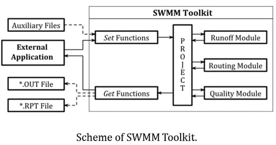
14] that allow using the model by an external application. This works as long as the network characteristics have been previously defined. The performance of the EPA SWMM program is sequential. First, an input module reads the files needed for the simulation. The network data are contained in an input or project file (INP file). These data might be complemented with auxiliary files for hot start conditions, weather data, etc. Then, if the analysis contains rain water data, a hydrologic calculation must be carried out in order to transform the rain in a runoff hydrograph. A hydraulic simulation follows, and then, if considered necessary, a follow-up on contaminant substances may be done in order to produce a quality model. All results are stored in a binary results file (OUT file). Finally, a report file (RPF file) containing some results statistics is written. The whole process is summarized on the right hand side of
Figure 1.
The performance of the interfacing functions provided with EPA SWMM follows the same structure, that is, as soon as the project is open, the input file must be read. Afterwards, the calculation is executed, thus being able to perform a step by step analysis. Finally, the results are written in a binary file that must eventually be read. This tool has 9 functions that can be used in order to manage the project. These functions are listed in
Table 1 as group 1. However, it is not possible to obtain partial results from the said simulation, or to perform data modification until the process is complete.
This performance mode was conceived in order to work with a different user interface, developed “ad-hoc” and well-integrated in other programs. Its most evident application would be the integration of the EPA SWMM engine within a geographic information system. However, the process is slowed down because of file access. On the one hand, it is required that the input file is written for every execution. On the other, in order to process results, EPA SWMM must write the results file and the external application should read it. These two operations require a great deal of programming efforts, and they may consume a significant amount of time.
An alternative to this performance mode is the development of a new set of communication functions. These new functions, integrated as a Dynamic Link Library (DLL), could address a wide array of problems present in applications and programming languages. The final objective is that, eventually, both EPA SWMM and any other application based on the EPA SWMM engine use the same library. An application that is external to EPA SWMM can therefore replace file use for information exchange, thereby ensuring time savings.
The Toolkit replaces the file reading and writing operations with two new groups of functions, as shown on the left hand side of
Figure 1. The first group–referred to as
Get Functions–is composed of functions associated with retrieving information either from project data or simulation results. The second group (
Set Functions) includes all the data modification functions. All the functions within this second group are simultaneously the most relevant and the most sensitive, since these functions will allow successive simulations by modifying data without having to access the files. For instance, by using the function
swmm_setLinkValue, it is possible to change the slope or the Manning roughness coefficient of a pipe during run time.
Table 1 summarizes the functions included in the Toolkit.
The optimal sizing of a storm water network might be taken as a first example. This issue is typically addressed by testing different combinations of diameters and slopes, which are ranked by using an objective function. The objective function includes the cost function for the new conduits and penalization terms when the constraints of the problem are not met. However, the whole problem has seldom been studied, even more so when considering the transient flow. Most authors have usually tackled this problem with oversimplified hypotheses. For example, in order to avoid having to perform a runoff analysis for every case, some authors use a constant inflow at network nodes instead of performing the hydrological model. Another example consists of using a steady flow model based on uniform flow. In this way, no duration is defined so that the calculation process is faster. However, it leads to the appearance of inaccuracies that increase with the size of the network and the discharge increase. Therefore, the steady flow model based on uniform flow is evidently insufficient when addressing situations for which surcharge or flooding risks exist.
If the temporal distribution of the rain water is included, then it becomes unnecessary to execute the hydrologic calculation every time. First, given the modular character of EPA SWMM, it is possible to execute a preliminary hydrologic calculation to obtain runoff hydrographs that enter in each element. With these inflows to the nodes, the hydraulic calculation can be performed as many times as it is required. The repeated modification of various network parameters will be necessary, but by using the Set functions, this no longer implies the constant rewriting of the input file. Because this operation requires a significant amount of computational time, the parameters will be modified directly in memory without accessing the writing of the files.
Finally, the binary results file EPA SWMM produces is not easy to manipulate. This file presents basic statistical summaries of the results (these summaries include items such as maximum discharges, maximum levels, volume balances, etc.). If more detailed information on a specific object must be obtained, the [REPORT] section on the project file must be modified to include this information in the result file, and then filter this latter file in order to look for the specific information needed. Since this process might be complex, it has become preferable to read the results obtained after each itineration. It is no longer necessary to read the result file, and the calculation process may be done faster.
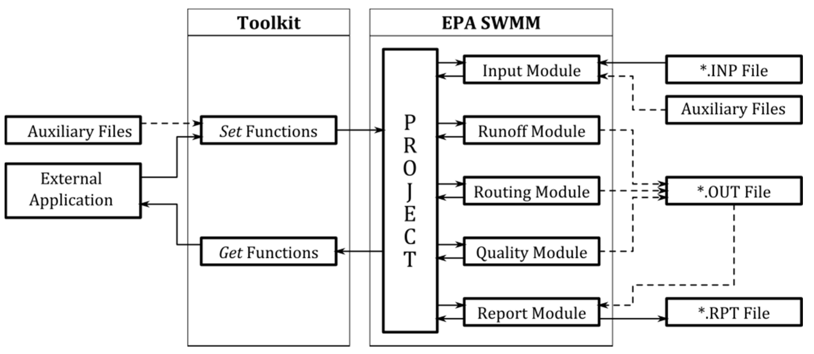
Figure 2 shows the flow chart of an optimization process that is based on the evaluation of an objective function. The left flow chart represents the process that is based on the EPA SWMM native interfacing tool. On the other hand, the right flow chart, instead, represents the same process but implemented using the Toolkit. It can be observed that several operations can be avoided. As the number of iterations increases so will the amount of time that is saved. Bear in mind that if evolutionary algorithms are preferred, the number of evaluations of the object function might be highly elevated.
3. Validation Protocol
3.1. Velocity Tests
Given that for simulations over extended periods, the calculation times can be relevant; this aspect has always constituted a preoccupation for the program's developers. The program was originally developed in FORTRAN [
15], with its successive adaptations. This way, when the original FORTRAN routines were converted to C language, the developers proceeded to make comparisons in terms of execution times [
16] as well as result precision [
17].
A series of tests will be done in order to support the previously mentioned statements. On the one hand, velocity tests have been carried out in order to measure calculation times for both options (EPA SWMM 5 Interface and SWMM Toolkit). A total of 9 cases in which network size, rain duration and rain-runoff simulation are modified have been performed for each option. Just as it was done during the SWMM 4-SWMM 5 transition [
16], and with the hopes of ensuring equality of conditions, every case was processed with the same computer.
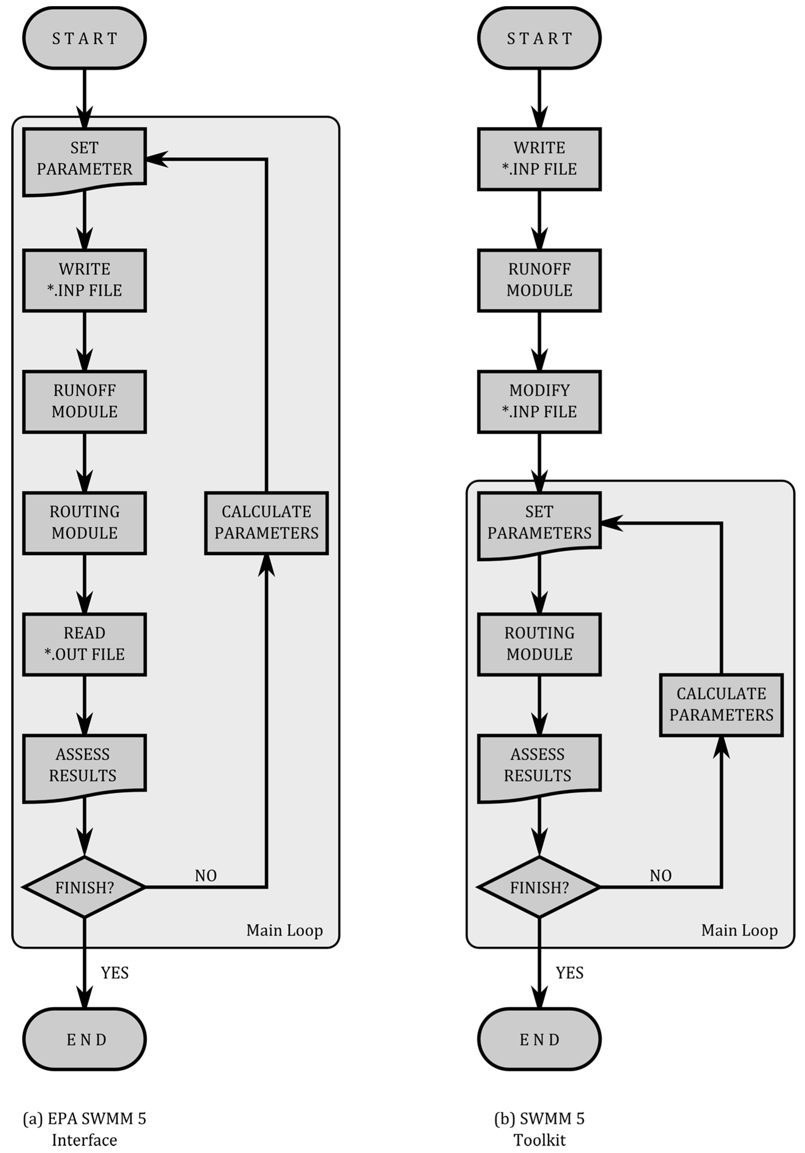
In order to see the effect that is obtained as a result of modifications in network size, three specific networks have been chosen and they are shown in
Figure 3. The first network (Net1) corresponds to the network that is available in the program’s manual [
14]. It is rather simple, as it consists of 5 nodes and 4 pipelines. The second network (Net2) is obtained by simplifying the sewer network of a district of Bogotá (Colombia) and consists of 82 nodes and 83 links. Finally, the third case corresponds to the Xirivella network (Spain). This network possesses all the elements that are typically found in a network, such as pumping stations, sewer overflows, waste water treatment plant, etc. It has 916 nodes and 931 links.
On the other hand, three different rain situations have been tested. In the first situation, once again the expected rain that is provided in the SWMM user’s manual sample is used. It consists of a 6-h long rainfall period, with intensity values that change every hour, and a 12-h long simulation. The second rain period corresponds to the data collected in a rain gage located in Almassora (Spain). All the records corresponding to October 2000 have been processed, with a 31-day long simulation and a rain time interval of one hour. Finally, for each of the three networks runoff, hydrographs obtained with the rain in case 1 have been collected. These hydrographs have been assigned as direct inflows in each of the nodes, and the hydraulic simulation has been done exclusively, thus avoiding hydrologic calculations.
In order to compare the differences in simulation times, the 9 cases (three networks × three rain events) have all been simulated using both the EPA SWMM native interface and the Toolkit. Execution times have been annotated for every case. For the comparison, a small application that allowed the measuring of the time employed in the calculation with millisecond precision was used. Ten simulations were carried out for each case in which some parameters such as slopes or diameters were changed. Total spent time was also measured for every simulation. The results of this test are shown in
Table 2.
It is possible to draw certain conclusions from the previous results. On the one hand, the greater the size of the network, the more time is required to calculate it. These data are obvious; however, it can also be observed that, the greater the size of the network, a larger percentage of time is spent in archive manipulation. When the Toolkit is used, there is a 25% time saving for network 1, 33% for network 2, and 77% for network 3 if the rain lasts 6 hours. It can also be observed that memory data manipulation slows down the process, that is, as the time that is destined for calculation increases, the relative importance of the time employed in archive data decreases. This is also an expected conclusion; however, when analyzing the results obtained in case 2, what is stated in the previous paragraph is ratified, since the Toolkit reduces the calculation time for a month-long rain by 0.2% for network 1, 4.2% for network 2 and 9.2% for network 3. Finally, the previous execution of the hydrologic calculation to write the results as direct inflow in a new archive supposes time savings of 10% in every case. Put differently, once the new archive without hydrologic data but with an entrance hydrograph for each node is obtained, the Toolkit may reduce calculation time by 10% when comparing this with the same operation using the EPA SWMM interface.
Short but intense rain periods are generally used in the optimization process, very similar to those seen in the case that was previously described. In these situations, one can observe how the Toolkit may significantly contribute to savings in calculation times. The larger the network, the more time saved. As has been observed, the saving may exceed 75% for very large networks.
3.2. Function Validation
Along its diverse history, SWMM has experienced numerous changes. The idea of the development team has always been that of maintaining reliability of the calculation, and this has been done through the implementation of a rigorous quality assurance testing program [
18]. In this case, the validation process has followed a similar philosophy to that used in the aforementioned quality assurance program, thereby guaranteeing the perfect coincidence of the results obtained with the Toolkit. This way, and just like it was done during the SWMM 4-SWMM 5 transition, three tests have been performed [
19]. These tests are based on two ideas.
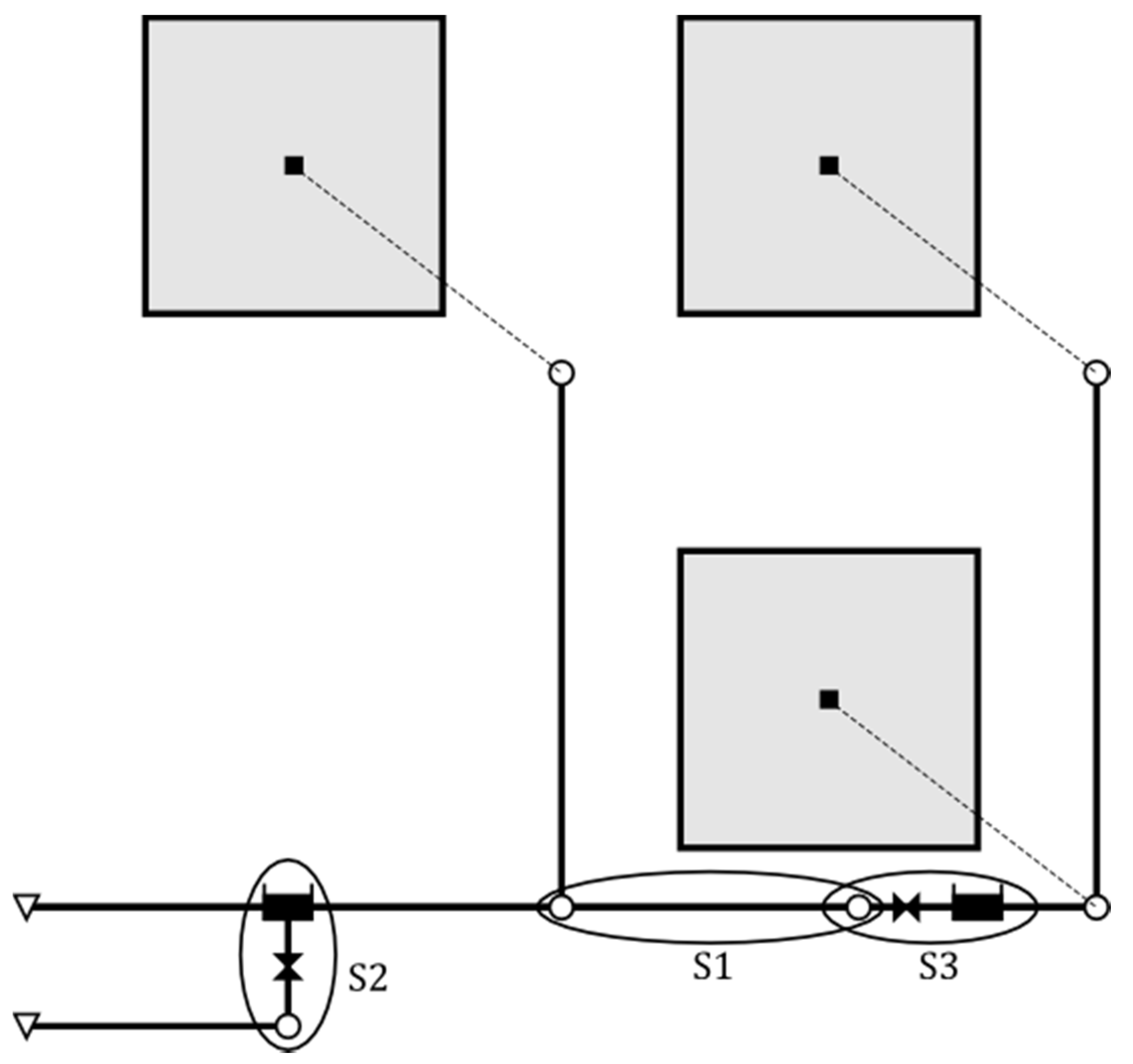
First, in order to ensure the compatibility of the Toolkit with EPA SWMM, a series of tests have been carried out to compare the results of both tools. The tests were conducted using the example network suggested in the SWMM 5 User’s Manual [
14]. This network is presented in
Figure 4, in which control sections S1, S2 and S3 have been established.
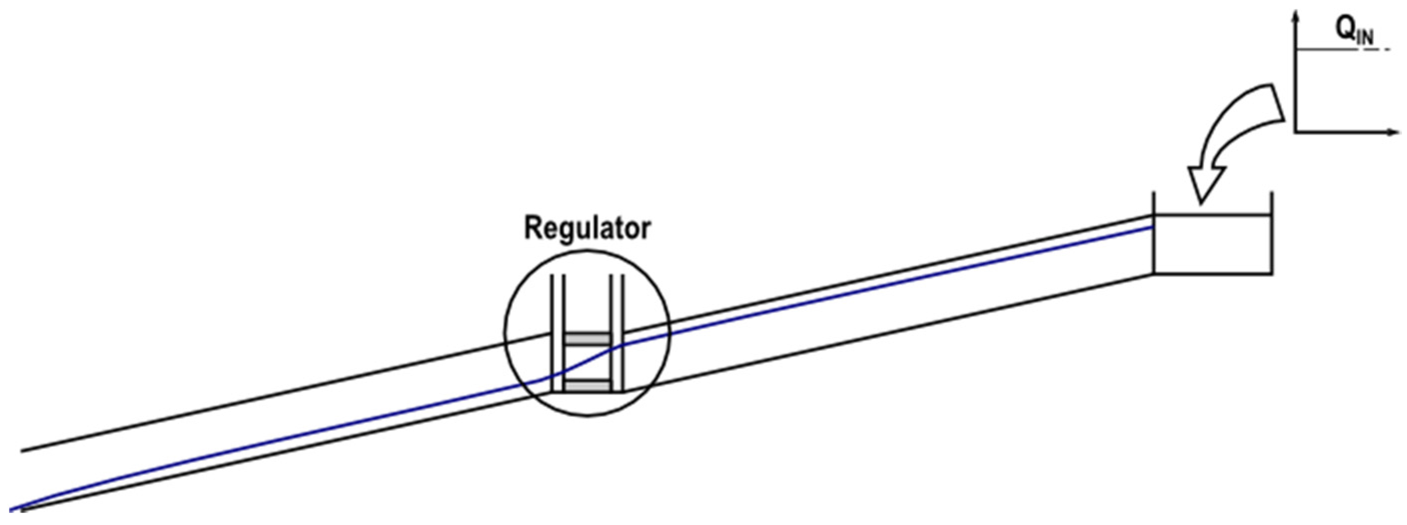
Second, a much simpler network was used to study specific control structures, as is the case of weirs, orifices and pumps. The reason for using a specific network for control structures derives from the way EPA SWMM calculates these types of devices. This way, different situations may be simulated (normal behavior, orifices behaving as a weir or weirs behaving as an orifice for surcharge conditions).
Figure 5 shows a sketch of this network, which consists of a storage unit with a constant direct inflow so that a steady flow regime may be reached. Likewise, the outfall is simulated as a free discharge. Conduits are long enough to allow them to reach the uniform flow in their middle points. Direct numerical calculations can thus be done, and they can be contrasted with those obtained with both EPA SWMM and Toolkit.
The tests could be grouped in two phases, depending on the functions that each of these tested. In the first phase, only the Get functions were tested, and only section S1 in
Figure 4 was used. The tests in this phase consisted of checking that the results obtained with EPA SWMM and the Toolkit are exactly coincidental without the need to manipulate information. The employed network was the one shown in
Figure 4 with a one-hour long rainfall and duration of the simulation of 12 h. The results corresponding to both nodes and pipes were consulted. During the first test, it could be observed that the Toolkit collected all the calculation instants. EPA SWMM, instead, only collected those results corresponding to the report time step. This way, a 10-s hydraulic calculation and report time step was employed in order to ensure equality of conditions. Likewise, in order to ensure the precision of the results, EPA SWMM preferences were modified, so that the reported results were always presented with a numerical precision of four decimals. Regarding the nodes, all the variables that could be read with the Get functions were processed, except for those related to quality water parameters. The same procedure was applied for pipes.
In the second phase, two sets of tests were carried out involving Set functions. These functions allow the integration of EPA SWMM with any other external applications including more complex algorithms of iterative character, such as design, control, or calibration algorithms. Because of this, tests have been more elaborate for this group of functions. Next, a brief description of each one will be done. The first set was carried out in section S3 of
Figure 4, and it included the basic elements such as storage units, junctions and conduits. The following parameters were modified:
Storage Units: invert level, height (maximum depth) y and volume. Regarding the volume, it is defined by a function which relates depth and surface area through three parameters: A, B and C. The surface area of the storage unit varies with water depth following the function shown below:
Junctions: invert level and maximum depth.
Conduits: diameter, invert levels at entrance and exit, and roughness coefficient. Furthermore, other tests were made in order to modify geometric shape and the corresponding geometric parameters. The latter tests were no so exhaustive as long as not all geometric shapes were tested.
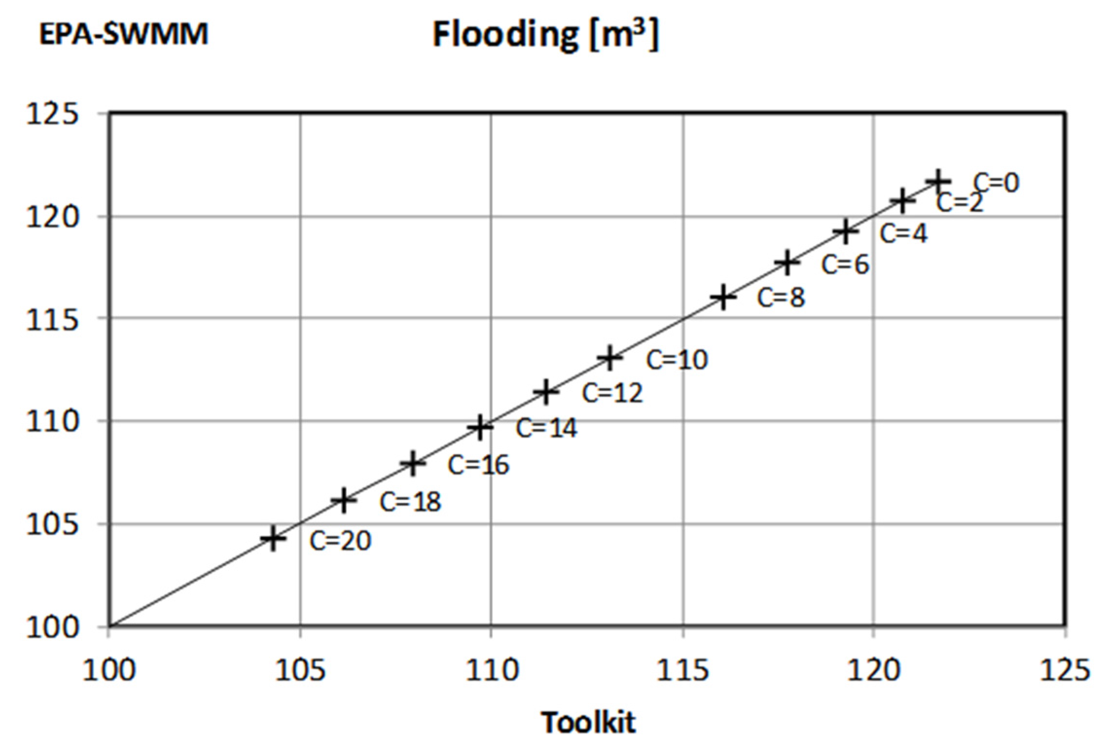
This set’s testing protocol will be briefly described. For each case within the set, three tests were carried out. The first included the analysis of the results obtained using EPA SWMM with a series of values of the analyzed parameter (10 different values ranging between a minimum and a maximum). Next, these same cases have been processed using the Toolkit and without parameter modification, that is, reading each of the 10 prepared archives. Finally, the obtained results have been analyzed by performing 10 calculations in one single process that used Set functions in order to modify parameters. As an example,
Figure 6 compares the results obtained when modifying storage capacity. The data collected for each of the storage volume include maximum discharges at entrance and exit pipes as well as total flood values for the initial and the final nodes. The results obtained through the use of the library have been represented on the horizontal axis. In the vertical axis, instead, those results directly obtained using EPA SWMM are represented. As expected, the results are 100% coincidental.
The second set was done for the exclusive study of control structures (orifices and weirs). Two networks were used on this occasion. Because it was important to use a section that would present discharge derivation, section S2 of
Figure 4 was used. The characteristics of these elements were modified by using the developed functions. This way, the performance of both elements was proven to be the same regardless of whether EPA SWMM or the Toolkit was used. The same behavior was seen in both cases.
Considering that control structures may become very important for applications such as real time control, a more exhaustive analysis was performed. In the case of orifices, EPA SWMM discriminates the case of flooding conditions (behavior as orifice) from that of not-flooding conditions (behavior as weir). Therefore, all the plausible situations contemplated by EPA SWMM were processed as a function of depths upstream and downstream of control element. The transition between the two performance modes is produced from a specific depth denominated critical height. Depending on the case, EPA SWMM implements a different coefficient and exponent. The network shown in
Figure 5 was used for this test. The detailed study that has been carried out helped to understand and perfectly reproduce the behavior shown by these control structures. As a conclusion, both EPA SWMM and the Toolkit presented the same results in all the cases that were analyzed.
4. Application
Usually, the design of a storm water network was solved by using the rational method. However, methods based on the concept of return period do not take into account economic issues. It might result in both overdesigned or underdesigned networks [
20]. Cost-optimal design of hydraulic network is a complex problem for engineers. Meredith [
6] applied dynamic programming to sewer studies including cost functions for pipes. Mays and Wenzel [
21] also used dynamic programming to optimize the design of a gravity sewer network with known pipe flow direction. Recent studies try to solve the problem of designing sewage networks by heuristic algorithms [
22,
23]. Furthermore, costs associated with flooding are rarely considered. Defining flood damage functions are another challenge for storm water network design [
24]. More recently, Guo
et al [
25] combined EPA SWMM with a cellular automata and genetic algorithm hybrid algorithm to design large sewer networks. In all previous studies, the inflows were considered constant. That is, the rainfall-runoff processes were not calculated. Furthermore, most of these studies considered a normal flow regime.
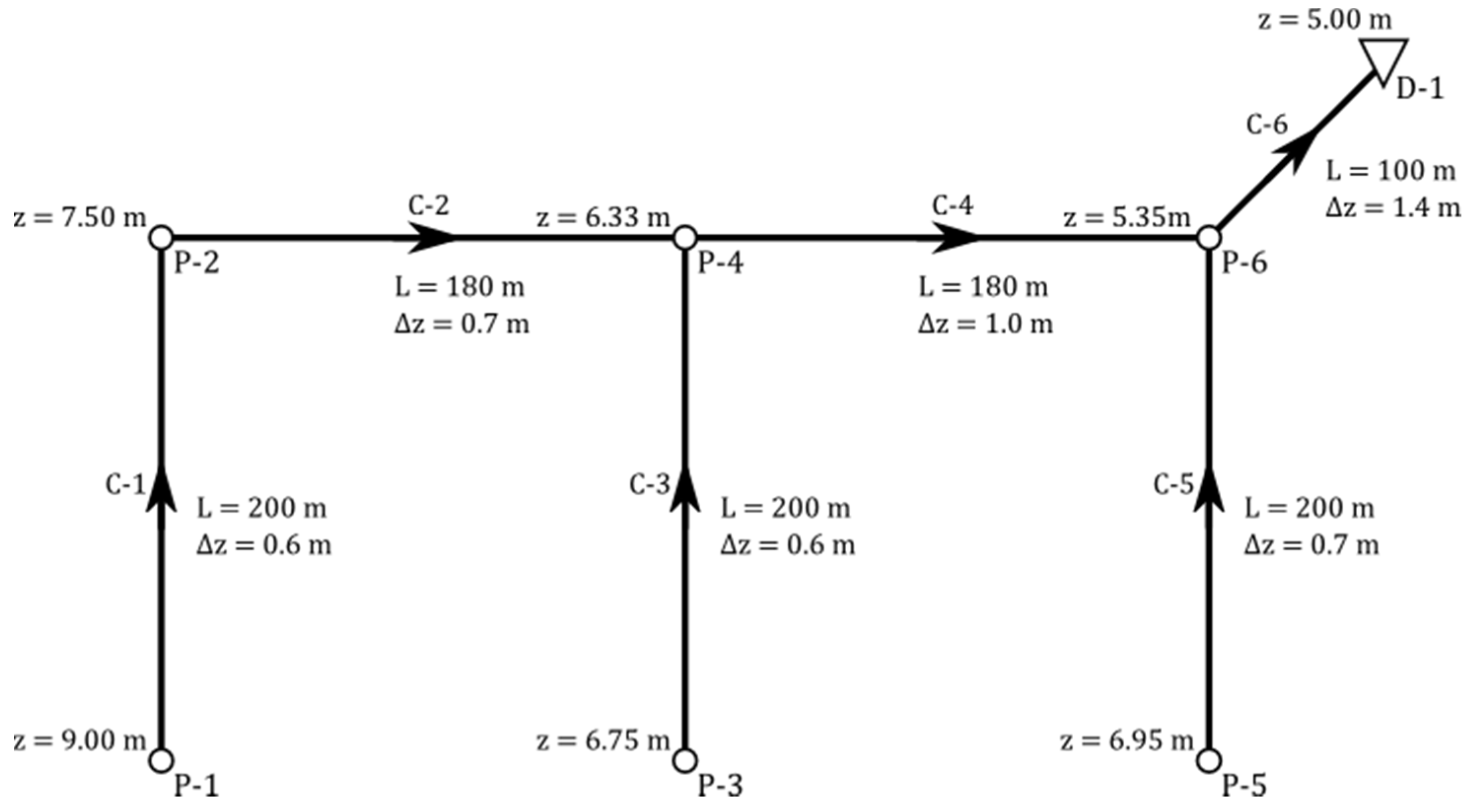
In this case study, the design of a simple sewage network is used as an example of application of the Toolkit. The dynamic wave approach is used for the hydraulic simulation. The network used for this application consists of 6 pipes, 6 manholes and an outfall. Node and pipe data are shown in
Figure 7.
Since the depth of the sewers should allow water flows by gravity, the design includes not only the dimensioning of the pipes, but also the depth at which these pipes must be installed. Hence, both the conduit diameters and their slopes must be calculated. It should be noted that diameters can be coded as discrete variables and they must be chosen among those listed in
Table 3. On the other hand, slopes are derived from the elevation and depth of the conduit ends. Therefore, they are continuous variables that may assume any value. As it happens in every design problem, constraints have been used for maximum velocity, capacity of the conduit and minimum slope. Another restriction was used, based on a similar one proposed by Meredith [
6]: the invert elevation of a pipe leaving a manhole cannot be higher than the lowest invert elevation of a pipe entering the manhole.
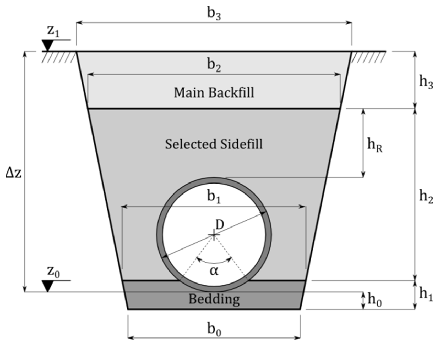
When calculating pipe installation costs, a formulation which involves both cost of the pipe according to
Table 3 and the cost of installing such a pipe. In order to do so, a standardized trench was used (shown in
Figure 8). It will depend on both the diameter (D) and the maximum depth the pipe can be installed (Δ
z). The trench model used is shown in
Figure 8, as well as all the data that defines it. It is worth mentioning that the same type of trench has been used for all the pipes, regardless of the type of terrain in which pipes were located.
This way, the data required to define the trench include:
Pipeline depth, Δz. It will be defined by the design algorithm.
Trench lateral slope, St. For this case study, this slope is considered constant and equal to 0.2 m/m.
Base width (b0). It is equal to pipe diameter plus 50 cm.
Bedding thickness (h0), also constant and equal to 15 cm.
Selected sidefill height (hR), measured from conduit crown level. Again, it is constant and equal to 30 cm.
Pipeline charge angle α. It indicates pipeline portion in contact with bedding. In this case, it is equal to 90°.
Ground elevation, z1
Invert elevation, z0
Likewise, z0 and z1 represent the invert and the ground elevations, respectively. The latter is calculated in the algorithm for all nodes with the exception of the outfall node D-1 for which z0 = 2.5 m. Therefore, using these values and pipe diameters it is possible to calculate the rest of the geometrical parameters of the trench.
With the trench parameters, it is possible to calculate the volumes that correspond to each part of the trench construction. These calculations must then be associated to the costs of the different actuations that were performed on the terrain. A cost function associated with the trench is thus obtained, which is the sum of the terms shown in
Table 4.
The geometrical calculation of the trench gives a cost function for pipe
i that depends on the diameter (
), the depth (
) and the length (
) of the pipe:
According to the object model of EPA SWMM, the elevation of both ends of each conduit will be computed and must be modified during the calculation process. Because of the different nature of the variables, two algorithms have been used for network design: a pseudo-genetic algorithm (PGA) and the particle swarm optimization (PSO) algorithm. PGA is a modified genetic algorithm that replaces the binary coding of each variable by an integer coding [
26]. Therefore, PGA is meant to address problems of discrete character. PSO, instead, is an algorithm more suitable for continuous problems [
27]. In both situations, modifications to the different generations have been performed with the help of the Toolkit functions.
In order to modify the slope of conduits, only the elevation of the downstream end of the pipe was modified, while the upstream end was fixed to the invert of the upstream node. The pipe slopes have been limited to be between 0% and 5%. The slope has been coded differently depending on the algorithm used. In the PSO method, due to its continuous nature, any value within this range has been allowed. In the PGA, instead, the range was divided into 100 intervals. This different coding is one of the reasons why PSO presents higher execution costs but better solutions than PGA.
Some restrictions were imposed. Maximum allowable velocity in pipes (
) was fixed at 4 m/s. As it is common in optimization problems with restrictions, if they are violated, penalizations will be applied to the cost functions. If the velocity in a pipe (
) is bigger than the maximum velocity, a binary variable
will take the value of 1 and the penalty will be the exceedance times the penalty cost (
). Finally, damage functions for flooding and surcharge conditions were assumed. As the target of the design was to avoid both situations, these functions were high enough to discard designs with flood or surcharge. Therefore, if the water level in node
j (
) is higher than the level that provokes surcharging (
), another binary variable
will take the value of 1 and a penalty cost (
) will be added. Then, the fitness of a solution
k will be given by an objective function
that accounts for the pipe costs and the penalties for constraint violations:
In this equation, is the cost of pipe i in solution k according to Equation (2), is the number of links and is the number of manholes in the model.
In order to account for computational costs, nearly 7000 simulations were carried out for every algorithm. All the simulations were done with an initial population of 100 individuals, and the rest of the parameters were tuned for each method [
28].
The optimal result obtained using the AG design model offers a solution that costs 290,441.68 €, while the solution obtained using PSO design model is 287,518.02 €. Both algorithms yielded the same solution for diameters, but since PSO is a continuous algorithm, its results are slightly better (1%) compared to those obtained by using APG. On the other hand, APG needs less than half the number of iterations than PSO. Furthermore, the rate of success of APG (as defined in [
28]) is better. The summary of these results can be seen in
Table 5.
5. Conclusions
The EPA SWMM program is a sewerage network hydraulic simulator that is widespread. However, its integration with other programs is quite limited [
5]. Because of this fact, a function library (known as a Toolkit) that allows the use of EPA SWMM algorithm in more complex calculation programs has been presented.
The principal objective of the present study is the development, testing and application of a functions library that allows the execution of multiple simulations with the EPA SWMM. This library must allow data modification and results querying without reading or writing files.
The library is made up of three different groups of functions. First, the project management functions will be enclosed in the group of interfacing functions provided by the USEPA within the program. The second group consists of those functions that are associated with data and result gathering. These functions can be referred to as Get functions. Finally, a data modification functions (denominated as Set functions) were included in order to give the library a greater degree of flexibility.
This library has been tested in order to show an improvement in simulation times. With it, one can avoid the writing of the data archive for every simulation. Likewise, the functions that are included in this library allow the incorporation of the hydrologic calculation’s results into the project’s data, and the writing of the binary archive as well as the results report has been avoided. In exchange, the results are kept in the memory with the resulting savings in the calculation times. All this has led to saving in calculations times, which in some cases has exceeded 75%.
Finally, the library has been subjected to a result validation protocol that proves the obtained results are 100% similar to those obtained with the original program. The functions that are included in the library have been directly contrasted with the results obtained with the original program, thus obtaining a perfect adjustment for every case. Furthermore, because the library allows the reading of results directly from the calculating tool, a rounding error is avoided as result precision increases. This way, results obtained from the validation process confirm 100% compatibility between those results obtained using EPA SWMM and those obtained by the external programs using the Toolkit.
Once validated, the library has been applied to the design of a sewerage network in which the diameter calculation and the slope adjustment have been combined. This is done by using a cost function expression that takes into account not only pipe acquisition costs but also the costs associated with pipeline installation as well (excavation, trenching and backfilling). For the development of the cost function associated with each diameter, a parameterized-type trench has been defined, one that can be used in other applications. The principal conclusion that can be drawn from this study case is that it is possible to combine the Toolkit with an optimization program that modifies the network data based on the results obtained from the simulation without the need to deal with files, thereby allowing time savings during the simulation.
In this comparison, two different evolution algorithms have been used: one for solving discrete problems (PGA) and another for continuous problems (PSO). This application was meant to contrast the Toolkit utility in more complex problems that were based on repetitive successions of a single simulation. As an additional result, it has been proved that the PSO algorithm (conceived for continuous variable problems) produces better solutions compared to those produced by PGA. However, PGA gets the best solutions with a lower number of simulations, that is, in a smaller time and more frequently. This conclusion confirms what has already been observed with other authors in continuous optimization problems [
29].
There is some field for future research regarding this work. The work was done in response to the problem of the design of a storm water network. Because of that, all the functions presented in this paper are related to hydraulic objects, that is, elements involved with hydraulic calculation. Hydrologic objects such as subcatchments or rain gages were not considered. Since the rainfall runoff process is another important part of the hydrological cycle, it would be interesting to extend the scope of this work to hydrological simulation. Finally, there is a growing interest in Sustainable Urban Drainage Systems (SUDS). EPA SWMM includes these systems and their design might be boosted with the help of similar functions for such a systems.
As a final conclusion, it can be said that the connection library with EPA SWMM represents a powerful tool for applications based on changing network parameters, as is the case of the formulation of sewerage network design. Besides, it allows saving of computational costs. All the aforementioned results allows the possibility of applying this library to other applications of different natures, which is precisely the case of the studies that are currently being implemented for sewerage network adaption to climate change.


 ,
, 


