Article

Water Availability of São Francisco River Basin Based on a Space-Borne Geodetic Sensor

1
School of Earth Sciences and Engineering, Hohai University, Jiangning Campus, Nanjing 211100, China
2
Department of Geomatic Engineering, Kwame Nkrumah University of Science and Technology, Private Mail Box, Kwmasi, Ghana
*
Author to whom correspondence should be addressed.
Water 2016, 8(5), 213; https://doi.org/10.3390/w8050213
Submission received: 3 March 2016 / Revised: 10 May 2016 / Accepted: 17 May 2016 / Published: 20 May 2016

Abstract

:
Brazil has recently experienced one of its worst droughts in the last 80 years, with wide-ranging consequences for water supply restrictions, energy rationing, and agricultural losses. Northeast and Southeast Brazil, which share the São Francisco River basin (SFRB), have experienced serious precipitation reduction since 2011. We used terrestrial water-storage (TWS) fields, inverted from the Gravity Recovery and Climate Experiment (GRACE) mission measurements, to assess and quantify the ongoing drought over the SFRB. We found a water loss rate of 3.30 km3/year over the time-span of April 2002 to March 2015. In addition, the TWS drought index (TWSDI) showed the extension of the recent drought that has jeopardized the SFRB since January 2012, and which reached its maximum in July 2015 (the end of TWS time series). In this sense there seems to be a linkage between the TWSDI (wetness/dryness) and the El Niño Southern Oscillation (ENSO), in terms of the wavelet coherence, at the semi-annual and biennial bands, suggesting a relationship between the two. While acknowledging that further investigation is needed, we believe that our findings should contribute to the water management policies by quantifying the impact of this drought event over the SFRB.

1. Introduction

Drought, as an extreme hydrological event, has serious impact on humanity. Impacts include loss of life, crop failures and food shortages, health issues, and mass migration [1] and the consequences on society and the environment are far reaching. For example, Tøttrup et al. [2] have reported the impact of drought at the Horn of Africa on the phenology of the songbirds’ migrations to Europe. The environmental effects of droughts in Amazonia, a very humid region, have included forest fires, reductions of biomass, and forest mortality [3]. Despite its impacts drought remains a major threat causing extensive damage to the environment and the economy around the world. The global effects of droughts and extreme heat have cut average national cereal production by 9%–10% with more damage in developed countries than developing ones [4].
Even Brazil, known as “the Saudi Arabia of water” due to its abundant renewable water resources, has faced chronic shortages of water availability over its metropolitan regions of São Paulo (20 million inhabitants) and Rio de Janeiro (12 million inhabitants). These two cities are the capitals of the homonymous states which are responsible for 43% of Brazilian gross domestic product [5]. Due to the droughts in Brazil, analysts have predicted potential massive loss in agriculture in the year 2014 which could reach millions of dollars [6]. The consequences of this prolonged water depletion jeopardize Brazil, a country of 206 million inhabitants and with a population growth rate of approximately 0.8% (estimated in 2004), with consequences far beyond the economy. For example, the ongoing drought has been associated with the outbreak of vector-borne (e.g., Aedes aegypti) diseases such as Zika fever [7,8] and dengue fever [9].
The 2013/2014 drought, which affected the southeast of Brazil, including the States of São Paulo, Rio de Janeiro, as well as Minas Gerais, has been described as the worst drought in 80 years [10]. This event has been attributed to an expressive precipitation deficit during the austral summer [11] leading to a number of impacts in the availability of water for human consumption, agriculture, and hydropower production. Coelho et al. [11] have reported on the possible relationship between the rainfall reduction observed in the summer 2014 in Southeast Brazil and the sea surface temperature (SST), as well as atmospheric circulation patterns. They demonstrated the persistence of a mid-atmosphere blocking high over Southeast Brazil during the 2013/2014 drought.
Historically, Northeast Brazil has been struck by many droughts. However, the 2012/2013 drought was one of the most severe in the recent decades [12] with more than 10 million people impacted in the semi-arid region. This extreme condition in the northeast was linked to the deficit of rainfall and drying conditions that contributed to reduced soil water availability [12]. The reduction of rainfall over those regions has been speculated to be due to anthropogenically-induced climate change [13] and deforestation in Amazonia [14]. Otto et al. [9] found limited support for this view, albeit that the possibility of human influence on the water crisis in Southeast Brazil was not completely discarded. Despite the need for further research on the causes of the reduction in precipitation, there appears to be little doubt (e.g., Getirana [15]) that the recent water depletion over Northeast and Southeast Brazil is mainly due to the lower precipitation rates.
The relation between precipitation ( P ) and other hydrologic quantities such as evaporation ( E , describing all process of vaporization) and the surface and sub-surface lateral transport of waters ( · R ) can be described in terms of the terrestrial water balance (TWB) as [16]:
S = t 0 t 1 ( P E · R ) d t
thus, any variation in the quantities of the right hand side of Equation (1), for example, precipitation, gives rise to changes in terrestrial water-storage ( S ; referred to hereafter as TWS). Changes in TWS affect climate and weather and, as such, a good indicator of abnormal hydrological conditions, such as floods and droughts [17]. However, long-term observations of TWS—the sum of water stored in soil, snow, surface and sub-surface reservoirs, and biomass—are still lacking in most parts of the world [18]. This applies especially to regions such as Africa and South America, where hydroclimatic datasets are mostly limited.
Global and local hydrological models provide a valuable tool in assessing TWS. However, the application of these models over a particular region generally relies on ground- and space-based measurements for inputs. The Gravity Recovery and Climate Experiment (GRACE) satellite mission has significantly changed this situation by measuring the Earth’s time-variable gravity field. This can be inverted to produce maps of TWS with a spatial resolution of approximately 333 km (at the equator) and temporal resolution of one month [19]. For instance, Andersen et al. [18] used GRACE-derived TWS fields to assess the droughts on central Europe in 2003. Since then GRACE-derived TWS has been applied as a viable alternative to ground-based observations for monitoring droughts in the continental regions. See, for example, [20,21,22,23,24,25,26,27,28,29] and the citations therein.
In the Brazilian context, GRACE-derived TWS fields have been used to characterize hydrological events in Amazon River basin (see, e.g., [21,22,24,25]) and over the La Plata River basin [23]. For instance, in [22], Chen et al. used GRACE-derived TWS for characterizing the 2005 drought event in the Amazon River basin. They have reported that data-assimilating climate and land surface models (namely National Centers for Environmental Prediction, NCEP, Reanalysis II and the Global Land Data Assimilation System, GLDAS-Noah, respectively) significantly underestimate the drought intensity. In [24], Frappart et al. analyzed the GRACE data and reported that the signature of the 2005 and 2010 droughts in the Amazon Basin in terms of spatial patterns and intensity. Their results are in good agreement with independent datasets (i.e., water levels, discharges, vegetation activity, forest fires, and drought index), which demonstrated the feasibility of GRACE to monitor large-scale droughts. Over the Brazilian Cerrado, Oliveira et al. [30] found that the TWS changes estimated by the TWB approach and those derived from GRACE show a significant correlation for all three watersheds within the region (i.e., Tocantins River basin, Paraná River basin, and São Francisco River basin). Their results indicated that GRACE data may represent the TWS change in the Brazilian Cerrado satisfactorily, allowing assessment of the seasonality of the water balance in this region. In a recent study, Getirana [15] used GRACE-derived TWS monthly fields for characterizing the water deficit in the regions of Southeast and Northeast Brazil, which share the São Francisco River basin (SFRB). He found a water loss rate of −61 mm per year (mm/year) over Southeastern Brazil during the period 2011–2015. The Southeast Brazil covers approximately 37% of the SFRB’s area while the Brazilian Cerrado covers about 57%, with the former being the main headwaters of SFRB.
In this particular contribution however, the focus is specifically on the SFRB, which has been hit by an unprecedented drought since 2012. Severe droughts have caused serious impacts on water supply and agriculture of the SFRB, especially during the rainy season [31]. Previous studies have taken advantage of the freely available precipitation fields to characterize the droughts over Southeast and Northeast Brazil using the Standardized Precipitation Index (SPI), see, e.g., [31,32,33]. However, the SPI does not account for anthropogenic impacts on the water availability of a particular region (or a river basin) such as increased irrigated agriculture, new reservoirs, regularization of discharge or water transfer projects, which are all characteristics of the anthropocene era [34,35]. As mentioned above Getirana [15] examined the regional-scale water deficit using GRACE-derived TWS fields. However, his study did not account for drought characterization for quantifying drought severity in terms of the water absent from the SFRB. Presented here is an analysis of the TWS depletion associated with this extreme hydrologic event over the SFRB and its potential relation with the El Niño Southern Oscillation (ENSO).

2. Materials and Methods
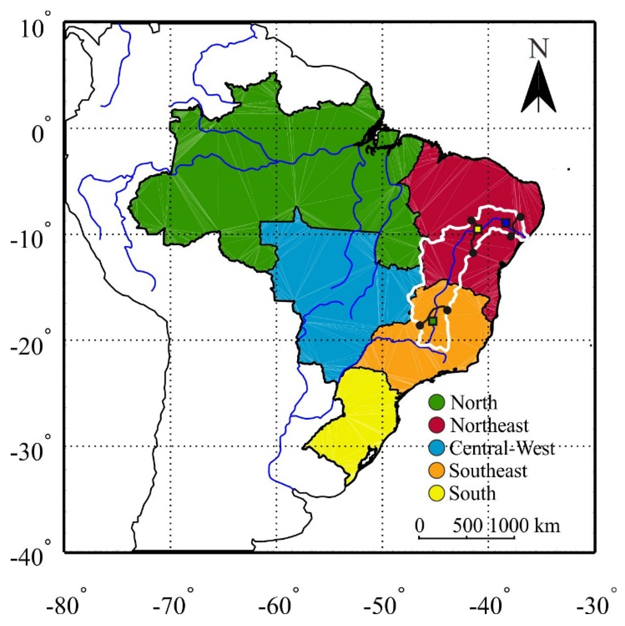
2.1. Study Area

2.1.1. Geography

The SFRB is located in Northeast and Southeast Brazil (Figure 1) and drains a total area of about 639,219 km2 (nearly 7.5% of Brazilian territory). Its main stream, the São Francisco River, has a total length of approximately 2830 km. The São Francisco River unites regions of great climatic, physical, environmental, and social diversity, in particular the southeast and the northeast. Hence, it is known as “the river of national integration”. It originates in the Serra da Canastra (Minas Gerais) in the central part of the Southeast region and finally washes into the Atlantic Ocean between Alagoas and Sergipe. The course of the river, running through five states, is divided into four physiographic regions: the Upper part (from the source up to Jequitaí, 17.2° S and 44.4° W); the Middle part (from Jequitaí up to Sobradinho Dam, 9.0° S and 40.8° W); the Lower-middle part (from the Sobradinho Dam up to Belo Monte, 9.8° S and 37.3° W); and the Low part (from Belo Monte to the river’s mouth on the Atlantic Ocean). A portion of the SFRB (~62.5%) is in the semi-arid region of the northeast, where the river accounts for roughly 2/3 of the freshwater availability. Additionally, SFRB has three reservoirs namely, Sobradinho (9.43° S and 40.83° W), Três Marias (18.21° S and 45.22° W), and Luiz Gonzaga (9.14° S and 38.31° W), where they account to 58.20%, 31.02%, and 6.62%, respectively, of the water used for power generation in the northeast.
The SFRB has an estimated population of approximately 17 million people, or about 8% of the Brazilian population, of which about 21% are considered poor by Brazilian standards [36]. Due to the basin’s enormous potential for additional economic growth, intense economic activities are exerting an ever increasing pressure on its natural and water resources. Of the 800,000 ha of land with potential for irrigation, more than 42% is being intensively irrigated. This is equivalent to about 11% of the irrigated area of Brazil and poses threats to sustainable water resource management. Consequently, efficient management of the SFRB’s water resources is of extreme importance for socioeconomic development of the region. This calls for regular monitoring of the variability of the SFRB’s hydrology, and the consequent impacts on its water resources to ensure sustainable use.

2.1.2. Climate

As mentioned in Subsection 2.1.1, the SFRB is vast and complex. It drains regions with precipitation greater than 1500 mm per year in its humid/sub-humid zones while in the semi-arid/arid zones of the Northeast this figure can be less than 350 mm per year. Fifty-eight percent of the SFRB lies within the area administratively described as the drought polygon, in the interior of the Northeast. The drought polygon’s water scarcity has fundamental natural causes such as extensive crystalline terrenes, annual oscillation of the Inter-Tropical Convergence Zone (ITCZ) and cyclical ENSO events. These are coupled with anthropogenic impact on the regional geography [37]. The main rainy season in the middle of the SFRB is during Nov-Dec-Jan (NDJ) with its maximum in December. In the northern portion of the SFRB, the main rainfall season is observed during February-March-May (FMM). This is linked to a high activity of the ITCZ with some heavy rainfall episodes associated with the passage of easterly waves and squall lines driven by the sea breeze (cf., Trejo et al. in [31] and the references therein). Conversely, the dryness over the northeast and north of the SFRB has been associated with an upper level cyclone over Amazonia [38]. Furthermore, Trejo et al. [31] found a high proportion of dry conditions during the main rainy season in the SFRB, which are attributed to specific partially-coupled atmospheric and oceanic patterns.

2.2. Datasets

2.2.1. Terrestrial Water-Storage (TWS) Monthly Fields

In order to verify the impact of droughts on the water resources of the SFRB, GRACE-derived monthly fields of terrestrial water-storage (TWS) were used. The temporal variations of the Earth’s gravity field as “sensed” by GRACE satellites are mainly due to the variations of the TWS after the atmospheric and oceanic mass variations are corrected for using de-aliasing products. The GRACE data used in this study are Level 3 (L3) products, which are gridded quantities estimating monthly changes of mass in terms of TWS at a spatial resolution of 1° (~111 km at the equator). These data are produced by NASA’s Jet Propulsion Laboratory (JPL) GRACE Tellus [39].
The data have been processed following the methodology developed by Landerer and Swenson as described in [39]. Basically, the monthly set of spherical harmonic coefficients (SHCs), which describes the Earth’s gravitational potential up to a certain degree and order (d/o) were filtered using a de-striping filter in order to minimize the effect of correlated errors which give rise to patterns of north-south stripes in TWS maps [40]. The SHCs were also filtered using a 300 km wide Gaussian filter in order to reduce additional high-frequency noise. The degree-1 coefficients were replaced by the values from the results provided by Swenson et al. [41], which represent the changes in the geo-center owing to mass redistribution in the Earth system. GRACE-derived degree-2 coefficients present high uncertainties. Therefore, they were replaced by those derived from satellite laser ranging as provided by Cheng and Tapley [42]. Neglecting the degree-1 coefficients would impact the amplitudes of annual and semi-annual variations of TWS estimates [43]. A glacial isostatic adjustment correction has also been applied based on the model provided by Geruo et al. [44]. In [45] Cox and Chao observed that the secular decrease in the degree-2 coefficients resulted primarily from the glacial isostatic adjustment, and is modulated by ocean and ice mass redistribution.
In [46], Klees et al. observed that the spatial smoothing reduces the noise and also introduces a bias (amplitude reduction) in the estimated monthly TWS fields. Thus a compensation due to the truncation of the SHCs up to a certain d/o (generally up to d/o 60, which is equivalent to a spatial resolution of ~333 km at the equator), de-striping algorithm and Gaussian smoothing were applied in terms of a gain factor as proposed by Landerer and Swenson in [39]. The gain factors ( k ; dimensionless), at each grid point defined by the latitude φ and longitude λ , were obtained through a least squares minimization as [39]:
[ Δ S u ( φ , λ , t ) k ( φ , λ ) Δ S f ( φ , λ , t ) ] 2 = minimum
where Δ S u and Δ S f is the unfiltered (“true”) and filtered (i.e., after being expanded to SHCs up to d/o 60, and filtered with a de-striping filter and Gaussian smoothing), respectively, water-storage time series at each grid point (1° × 1°) simulated by the Global Land Data Assimilation System (GLDAS) drives the Community Land Model (CLM4.0) version 4.0 [47]. The relationships between filtered and unfiltered TWS (simulated) at each grid point (1° × 1°), expressed in terms of gain factors k , which are independent of the actual GRACE data, can be used to extrapolate the GRACE-derived TWS fields from their nominal spatial resolution (~333 km, depended on the maximum d/o used as well as the filter scheme) to a finer spatial scale (here, 111 km due to the simulated TWS fields from CLM4.0 driven GLDAS used to compute the gain factors). Overall, the gain factors considerably reduce leakage errors, which arise from the GRACE post-processing filters [39]. Considering each TWS grid node as TWS( φ , λ , t ) where t is time (month), and the gain factor grid as k ( φ , λ ) , then the gain-corrected time series TWS′( φ , λ , t ) is simply:
TWS * ( φ , λ , t ) = TWS ( φ , λ , t ) k ( φ , λ )
TWS*, gain-corrected fields with 1° × 1°, from this point on will be designated as TWS.
It is worth noting that, the gain factors only give the relative signal attenuation and restores the signal to its “original” form and when working with other gridded datasets (e.g., soil moisture fields from GLDAS) it is not necessary to filter them as it is with GRACE data. Despite being an easy and comprehensive way to restore the signal losses in GRACE-derived TWS fields, the gain-factor as estimated by Equation (2) relies on the quality of the simulated TWS. For example, Long et al. [48] have shown that neglecting natural and human induced groundwater storage changes, and the interactions between surface and sub-surface waters compromises the effectiveness of the gain factor. To this end, many methodologies are available (cf., Long et al. [48], and references therein) for dealing with the leakage effects on GRACE-derived TWS.
The monthly L3 products are distributed in three versions computed using the solutions provided by the three centers of the GRACE Science Data System (SDS), i.e., the University of Texas Center for Space Research (CSR), the NASA Jet Propulsion Laboratory (JPL), and the Deutsches GeoForschungsZentrum (GFZ). Despite CSR solution provides the best results for the SFRB [49], as recommended by Sakumura et al. [50] and Xiao et al. [51], an ensemble solution was calculated as an arithmetic mean of the three data products (CSR, JPL, and GFZ). The ensemble solution is effective in reduce the noise in comparison with the individual solutions. To this end the time-span of the GRACE L3 data ranges from April 2002 to July 2015 (with the mean value of 2004–2009 removed) and linear interpolation of missing periods (June 2002, July 2002, June 2003, January 2011, June 2011, May 2012, October 2012, March 2013, August 2013, September 2013, February 2014, and December 2014). The reason for removing the mean field is that it is dominated by the static density distribution inside the solid earth and additionally the contributions from the mean stored water are also removed [16]. Thus, only the time-variable component of the water-storage can be recovered, i.e., TWS anomalies.

2.2.2. Bivariate ENSO Time Series (BEST)

The Bivariate ENSO Time series (BEST), which is derived from Niño 3.4 and Southern Oscillation Index (SOI) was used to describe the ENSO phenomenon (for details on BEST, we recommend the work of Smith and Sardeshmukh in the reference [52]). BEST combines the atmospheric (SOI) and oceanic (Niño 3.4) components of the ENSO processes into a single field, and thereby providing a more realistic characterization the phenomenon and was retrieved from http://www.esrl.noaa.gov/psd/data/climateindices/list/.

2.2.3. Tropical Rainfall Measuring Mission (TRMM)

TRMM is a joint mission between the United States (NASA) and Japan (JAXA, Japan Aerospace Exploration Agency) aiming to study rainfall for weather and climate research [53]. TRMM is designed for monitoring rainfall in the latitude range of ±50°. In this study, the monthly averaged 3B43 V7 rainfall products with a spatial resolution of 0.25° were used. The data were obtained from NASA’s Goddard Earth Sciences and Data and Information Service Center (GES DISC) available at http://mirador.gsfc.nasa.gov/. The data have been used in several studies of rainfall over Brazil, see, e.g., Melo et al., 2015 [54], and specifically over SFRB [30]. Note that, for a direct comparison of TWS time series and precipitation, it would be necessary either to integrate the precipitation rates [55] or derive the TWS [16] with respect to the time. If one wished to compare TWS (mm or km3) with precipitation rates (mm/month), a phase shift of at most three months, with respect to the maxima, would be likely (i.e., considering the signal described by harmonic, e.g., sine, waves).

2.3. Methodology

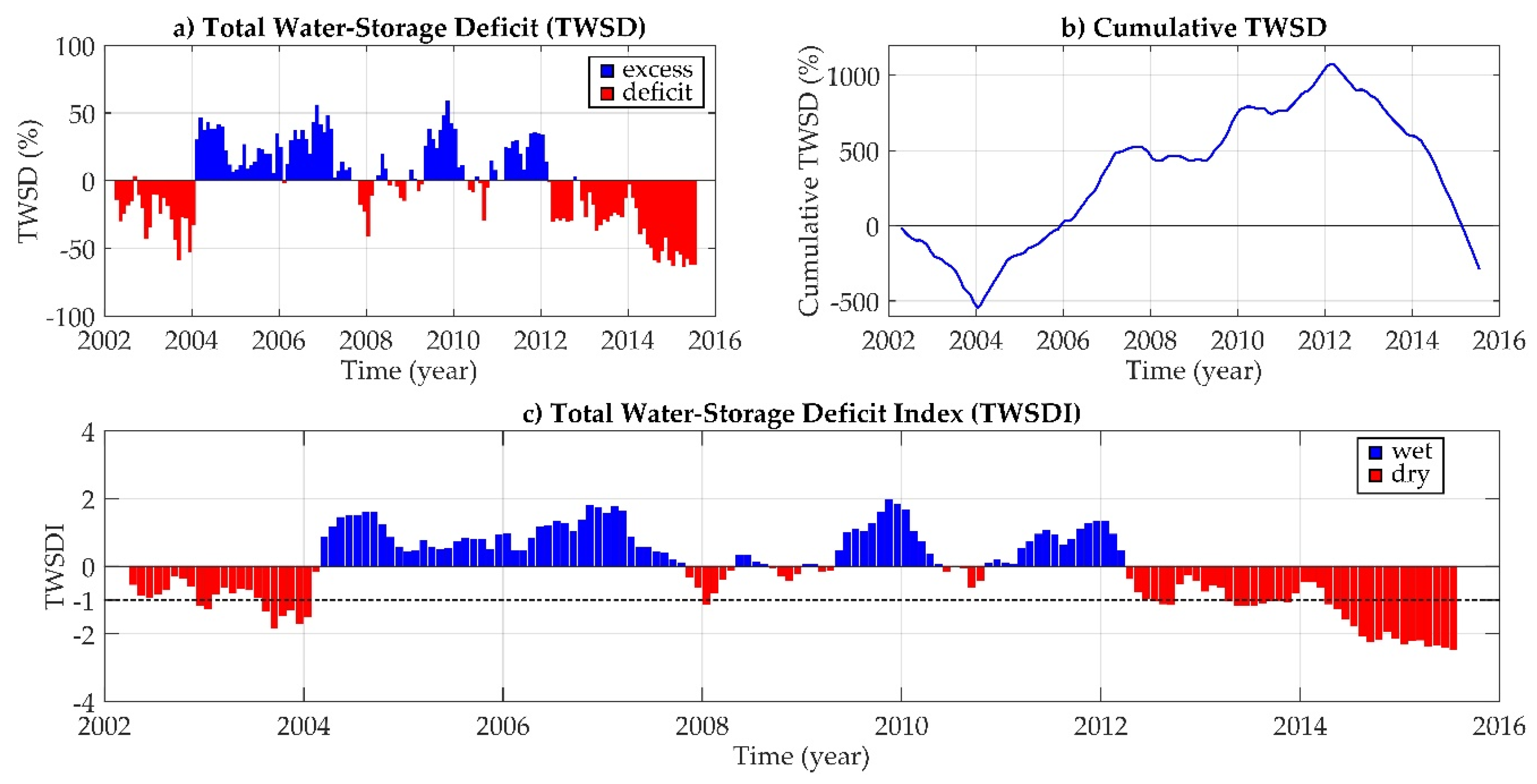
2.3.1. Total Water-Storage Deficit Index (TWSDI)

In [56], Narasimhan and Srinivasan developed a Soil Moisture Deficit Index (SMDI) based on weekly soil moisture. Yirdaw et al. [20] renamed the earlier SMDI as Total Storage Deficit Index (TSDI). Hereinafter it is renamed as Total Water-Storage Deficit Index (TWSDI), which is suitable for GRACE-derived TWS and its application on drought studies. It is important stress that, TWS differs from the soil moisture storage, which is utilized in SMDI. Using the long-term median, maximum and minimum TWS, monthly percentage terrestrial water-storage deficit (or excess) can be computed as [56]:
TWSD i ( % ) = TWS i median ( TWS j ) max ( TWS j ) min ( TWS j ) × 100
where TWSD i is the total water-storage deficit (%) and TWS i is the monthly total water-storage anomaly inverted from GRACE measurements (see Subsection 2.2.1), median ( TWS j ) , max ( TWS j ) , and min ( TWS j ) are, respectively, the long-term median, maximum, and minimum TWS monthly anomaly (i.e., with the mean removed from each monthly value of TWS, see Subsection 2.2.1) and with i = 1 to 160 (160 months from April 2002 to July 2015) and j = 1 to 12 (12 months of the calendar year). The seasonal median, maximum, and minimum were computed for the period of April 2002 to March 2015 (covering an integer number of years) in order to prevent the effects of strong seasonal signals from skewing the TWSD analysis.
The drought index can be calculated on an incremental basis as suggested by Palmer [57]. In this sense, the TWSDI can be calculated from the previous drought index and the current TWSD as [56]:
TWSDI i = 0.5 TWSDI i 1 + TWSD i 50
the initial value of TWSDI i 1 , that is, TWSDI 0 , is computed by multiplying the TWSD for the first month by a value of 2% as suggested by Narasimhan and Srinivasan [56]. TWSDI during a particular month ranges from −4 to +4, which represent the dryness and wetness conditions, respectively. Note that, the coefficients 0.5 and 1/50 (0.02) in Equation (5) are the duration factors p and q , respectively. They can also be determined based on the drought monograph, which is the best-fit line (in the least-squares sense) to the cumulative TWSD curve for the period of dryness. See Equation (12) of Yirdaw et al. [20] and the explanations therein.
Other TWS-based drought indexes have recently been proposed. For instance, Yi and Wen [27] proposed the GRACE-based Hydrological Drought Index (GHDI) for drought monitoring. However, the computation of GHDI also depends on the long-term mean soil moisture storage for the region. This can be retrieved from hydrologic model [47] or from space-borne sensors [58]. In [26] Thomas et al. have proposed a new metric in order to quantify the hydrological drought severity which, they claim, is applicable globally for drought characterization. Their approach is based on the residuals after subtracting the TWS normal hydrological condition of TWS (seasonal cycle) from the TWS time series. This is somewhat equivalent to the numerator of Equation (4) and the analysis proposed in the early work of Chen et al. [21]. In [24], Frappart et al. as also suggested standardized anomaly index of TWS based on the early work of Lamb [59] and it is slight different from Equation (4) since the extreme is considered with respect to the geographic domain of the target area, and not with respect to the averaged time series as it is in this study.

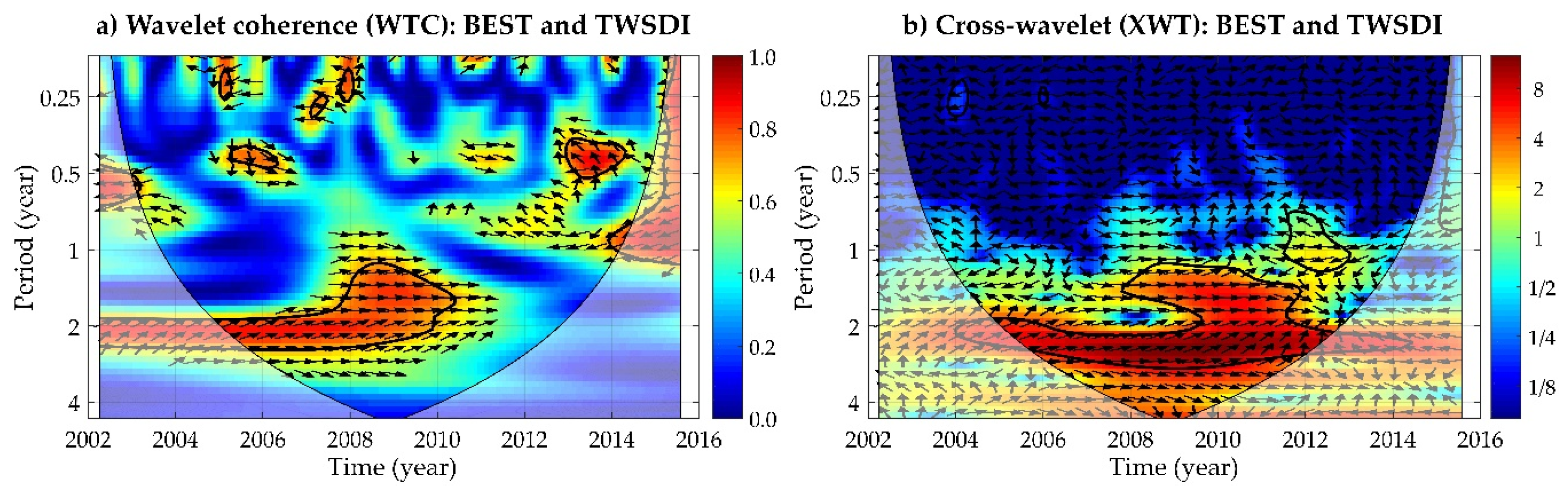
2.3.2. Cross-Wavelet Transform and Wavelet Coherence

It is worth be mentioned that most of the signals encountered in hydrology (e.g., rainfall, streamflow) have transient features, which lead to non-stationary processes. Thus, the use of wavelets, or time localized basis functions, can be used to decompose signals containing time-localized events. Hence. the cross wavelet transforms (XWT), which is capable of revealing regions in the time-frequency space in which two nonlinear time series have a high common power with a consistent phase relationship [60], were used to analyze the TWSDI and ENSO (BEST) time series. By its ability to provide such information, XWT can be used to discover causative relationships between time series. The cross-wavelet transform of two time series x n and y n , is given as [60]:
W = W x W y *
where * denotes a complex conjugation. Consequently, the cross-wavelet power is defined as the magnitude, W x y whiles the complex argument, arg ( W x y ) reveals the local relative phase between the two fields in the time frequency space.
Similarly, wavelet coherence (WTC) is adopted to reveal local non-stationary coherence between pairs of the time series used in this study [60]. WTC between two continuous wavelet transforms (CWTs) is useful to locate significant coherence against a background of red noise. The WTC between two signals is given as [60]:
R n 2 = | S [ s 1 W n x y ( s ) ] | 2 S [ s 1 | W n x ( s ) | 2 ] · S [ s 1 | W n y ( s ) | 2 ]
where S is a smoothing operator, s is the wavelet scale, W x y , the cross wavelet transform between the two CWTs, W x and W y , representing the two time series (e.g., ENSO and droughts). WTC can be seen as a localized correlation coefficient in a time-frequency space [60].

3. Results

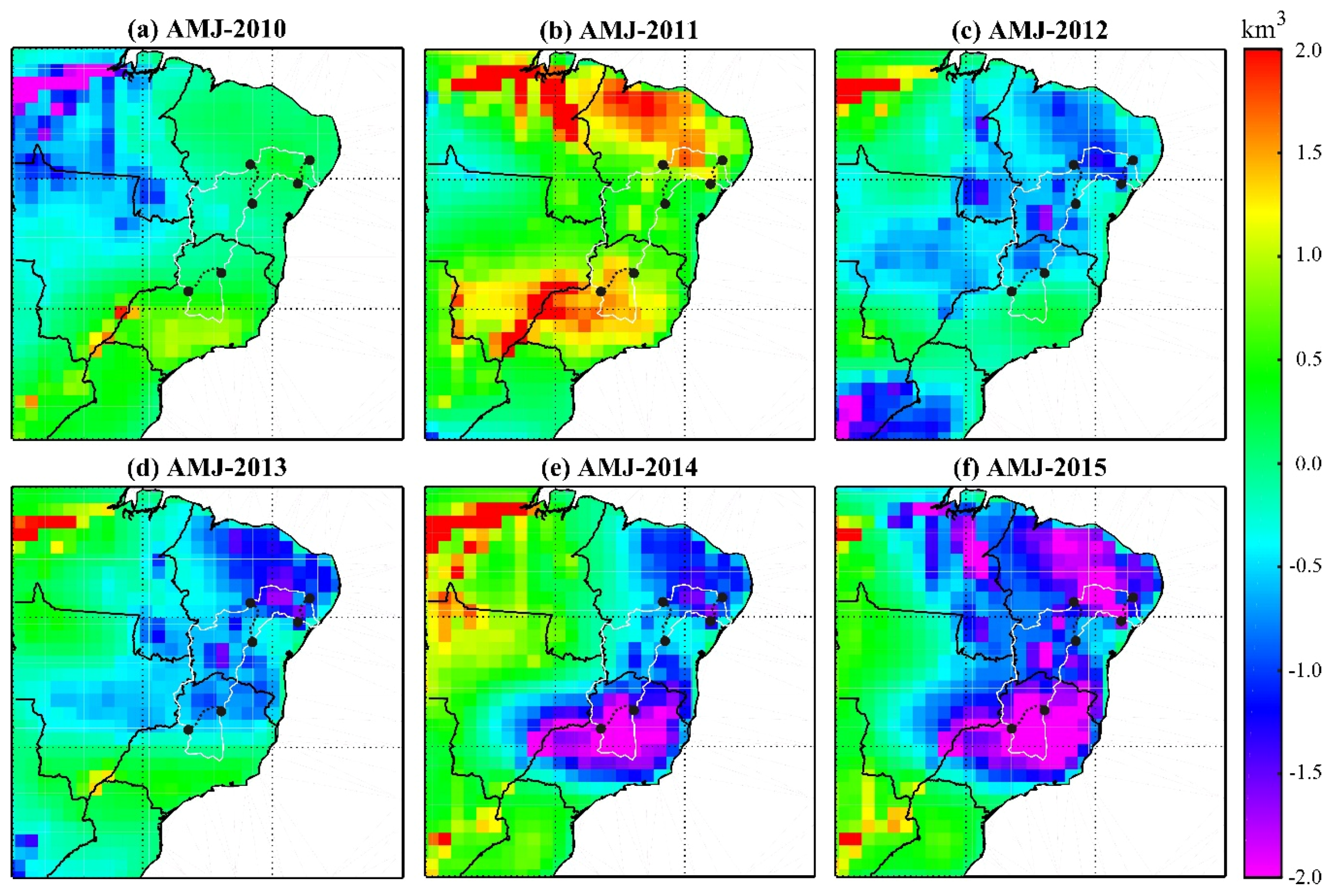
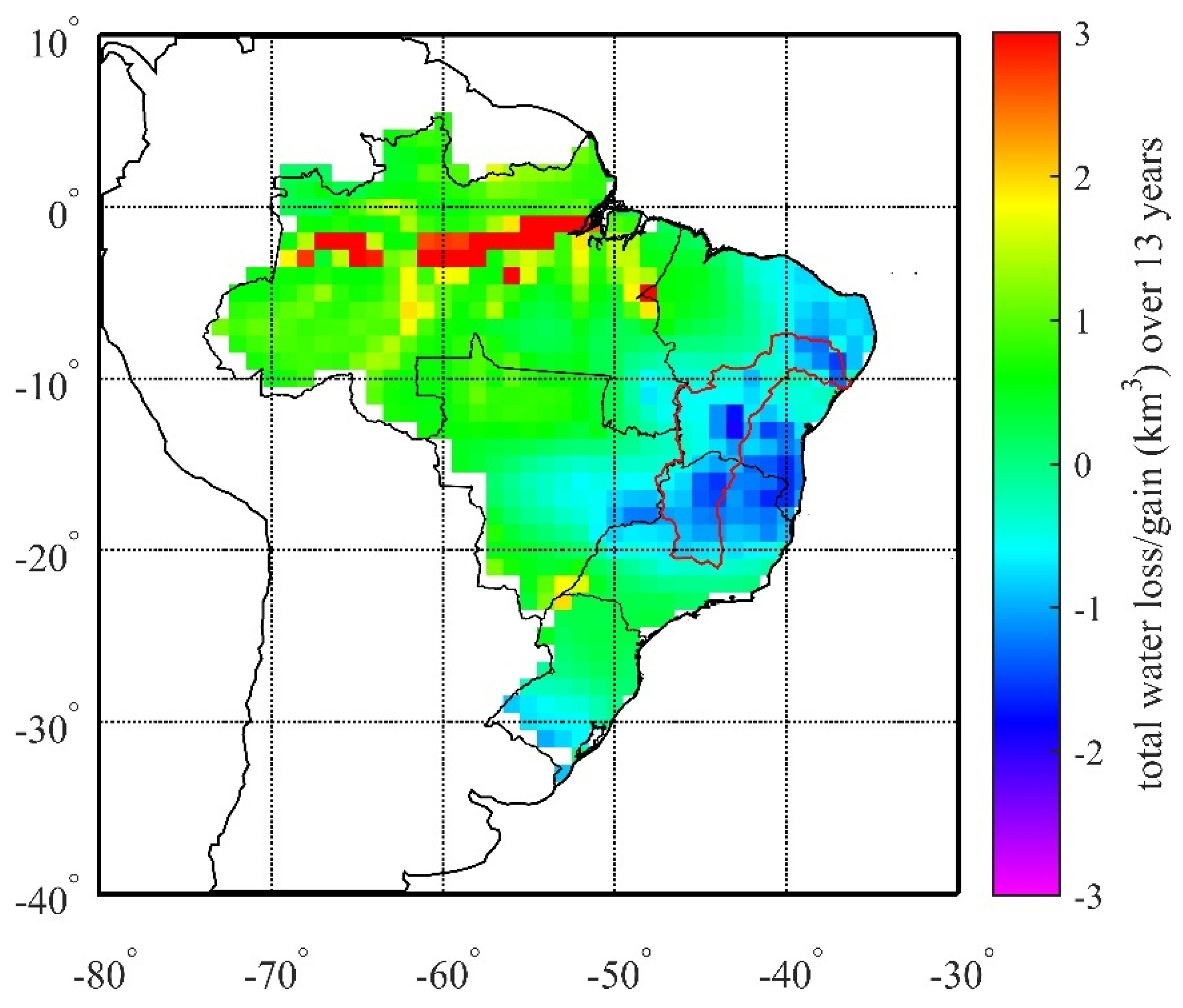
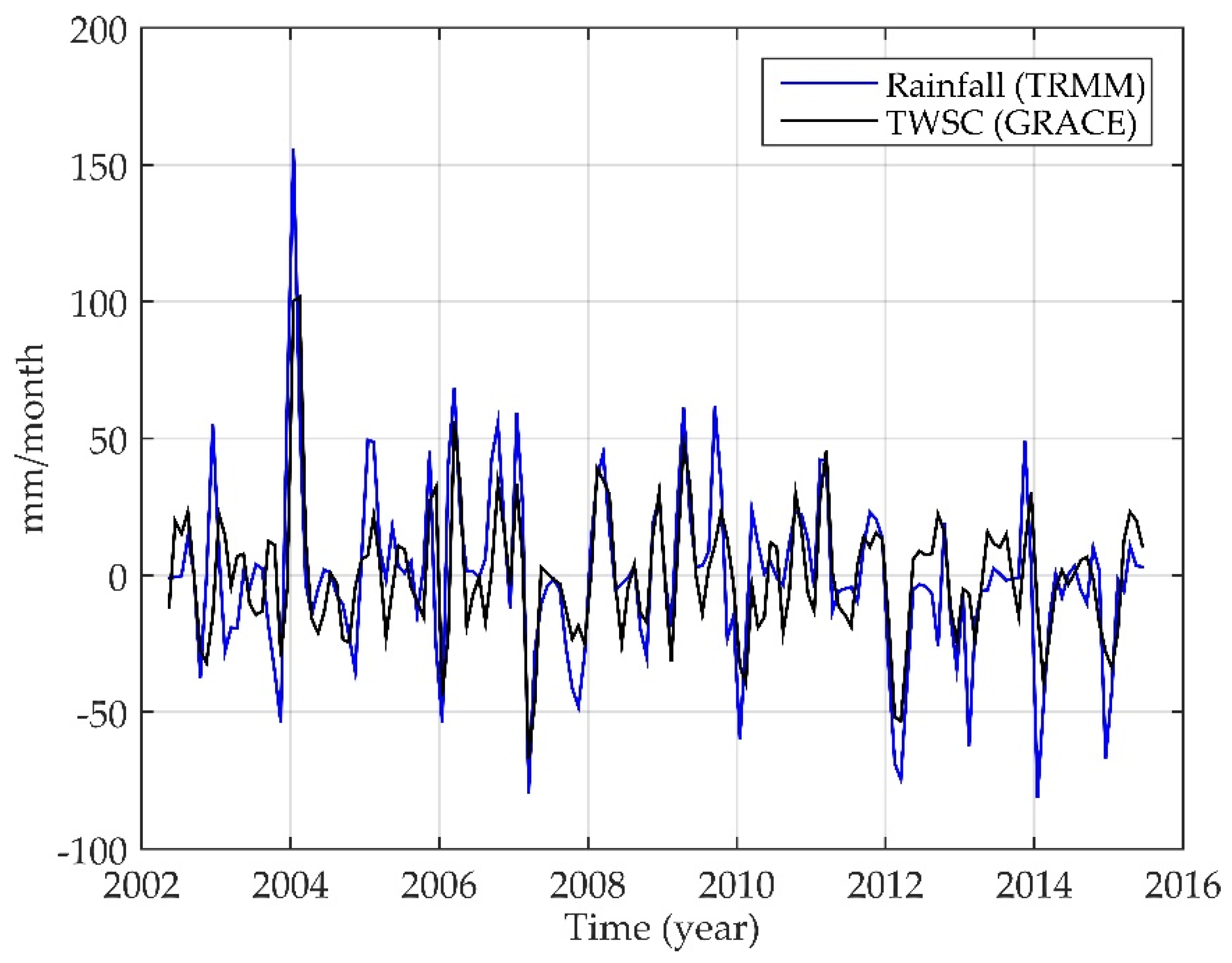
3.1. Variations of TWS

Following the computation of TWS fields (Subsection 2.2), a Mann-Kendall trend analysis and non-parametric Sen’s slope estimates were carried out on the TWS series at each grid point (1° × 1°) to detect monotonic trend direction and magnitude of change over time. The Mann-Kendall test is non-dimensional and quantifies only the direction of trend, hence, in order to quantify the true slope of an existing trend, the Sen’s non-parametric method was used. For more details on Mann-Kendall trend analysis and Sen’s slope estimations, see the reference [61]. The spatial pattern of total water-storage gains or losses estimated from GRACE data for Brazil covering the period of April 2002 to March 2015 (13 years of time span) is shown in Figure 2 in units of km3. The time span of April 2002 to March 2015 (i.e., covering an integer number of years) was chosen in order to prevent aliasing effects of strong seasonal signals from falsifying the time series analysis (see, e.g., Baur and Sneeuw [62]). The most obvious water-storage losses within Brazil are located in northeast and southeast regions. It is also possible to see the overall water loss within SFRB (delineated by the red solid line) over the time-span of 13 years detected GRACE, which shows a significant TWS loss of up to about −2.5 km3 in the Upper and Middle parts of the SFRB.
A regional average of the TWS time series within a particular region can be computed using [63]:
TWS ¯ ( t ) = 1 A i = 1 n TWS ( φ i , λ i , t ) A i
where n is the number of cells in the interior of a particular region (e.g., a river basin), A i is the area of the cell i and A is the total area of the basin. Note that A = i A i , thus the total area of SFRB using the grid resolution of 1° × 1° is different from the value presented in Subsection 2.1.1 (639,219 km2) due to the discretization. Accordingly, using Equation (8), the regional averages of the GRACE-derived TWS time series for the SFRB (Figure 3, top panel) were computed. There are variations due to the seasonal effects in the areal averaged TWS within the SFRB showing that the high water seasons occurs normally in April, with the low water season occurring in October. Furthermore, the variations of the TWS time series indicate a dry trend of −3.30 km3/year (significant at 95% confidence level) over the time window of April 2002 to March 2015. This is equivalent to a total volume loss of 43.77 km3 over the 13 years across the SFRB.
As in Thomas et al. [26] and Getirana [15], the 160-month climatology (April 2002 to July 2015) for the TWS time series, which were computed by averaging the TWS values of each month (e.g., all Januaries in the ~13-year record were averaged), were removed from the TWS time series of the SFRB (Figure 3, bottom panel). It is possible to identify two periods where the de-seasoned TWS time series are below zero (Figure 3, bottom panel). This de-seasoned TWS series seems to indicate water deficit over the periods April 2002 to January 2004 and March 2012 to July 2015. The first period (April 2002 to January 2004) presents an average value of −26.36 km3 and the second period (March 2012 to July 2015) an average of −39.46 km3, both signifying periods with months drier than the normal seasonal cycle of TWS within SFRB. The linear rate over the period of March 2012 to July 2015 is −17.63 km3/year, significant at 95% confidence level. The driest period portrayed in the residual TWS time series is February 2015 with −103.13 km3. The period of February 2004 to February 2012 presents an average value of TWS 22.66 km3 indicating a period wetter than the normal average. Indeed, the overall behavior of water availability in the SFRB is also depicted in its main reservoirs, Três Marias, Sobradinho, and Luiz Gonzaga (Figure 4a–c, respectively) in terms of useful volume (%) provided by the National Electric System Operator (ONS; Operador Nacional do Sistema Elétrico) of Brazil (http://www.ons.org.br/home/index.aspx).
The Sobradinho Reservoir (Figure 4b), the largest reservoir of the SFRB and the Northeast Brazil, went through one of the worst droughts within the time span of January 2002 to December 2015. Sobradinho Reservoir is responsible for 58.20% of the water used for power generation in the Northeast. In Figure 4b it is possible to see that the lowest useful volume is around November 2015 with 1.11%. The overall water depletion situation of the other two reservoirs within SFRB, i.e., Três Marias and Luiz Gonzaga, is the same where the 2012–2015 dry period is evident in terms of surface water storages. The SFRB’s water resources correspond to 96.86% of the water used for power generation in the northeast where Sobradinho Reservoir contributes to 58.20%, Três Marias Reservoir to 31.02%, and Luiz Gonzaga Reservoir to 6.62% (other basins contribute to 3.14%). In order to assess if GRACE is sensitive to the gravitational attraction of the water-mass variations of the reservoirs due to the impoundment of water, GRACE-TWS fields were averaged over a quadrangle area of 3° × 3° centered at the mid-point of the reservoirs (Figure 4d–f), for example, Sobradinho Reservoir ( φ 9.5 °   S and λ 40.5 °   W ). In this context, the volume conservation as:
A Q h Q = A R h R
was used to convert the water level of the reservoir h R into equivalent water layer h Q spread over the quadrangle area A Q . The water level variations of Sobradinho Reservoir were obtained from United States Department of Agriculture (USDA), Foreign Agriculture Service, covering the time period of July 2008 to April 2016 based on Jason-2/OSTM altimetry mission [64]. The time series were re-sampled to monthly values as those of GRACE (Figure 4, panel e). For Sobradinho case, the two series (GRACE and Satellite Altimetry) present a correlation coefficient of 0.86 with high statistical significance (p-value 3.75 × 10⁻²⁶).
The patterns of water-storage deficit from 2010 to 2015 computed as the average of the de-seasoned TWS (i.e., after removing the climatology means) over the months of April to June (AMJ) are shown in Figure 5. AMJ is the austral fall period [15] that follows the rainy summer season over Northeast and Southeast Brazil. It is possible to see the water deficit over the years of 2012 to 2015, which characterize the water depletion that has plagued the northeast and southeast as well as the SFRB. The impact of water depletion on these regions resulted in an abrupt decrease of TWS since 2012. However, the Upper part of the SFRB shows the strong impacts of the 2014/2015 drought events that jeopardized the water availability over the entire basin (see Figure 5). This is demonstrated by the fact that the source of the São Francisco River, which is located in the Southeast region at Canastra Mountain in the state of Minas Gerais, dried up completely in 2014. Though it does not represent the total volume of water in the SFRB, nonetheless it portrays the overall water crisis of Southeast Brazil. These negative anomalous storages represent the drought period that occurred in this basin and were well captured by GRACE satellite mission.

3.2. Terrestrial Water Storage Deficit Index (TWSDI)

Using Equation (4) the seasonality inherent in TWS of the SFRB was removed and the series was then normalized yielding values ranging from −100 to +100 i.e., very dry to very wet conditions [56]. The time series of the GRACE-derived TWSD is shown in Figure 6a. Note that the TWSD series (Figure 6a) and de-seasoned TWS (Figure 3, bottom panel) show almost the same information in terms of water availability within SFRB with respect to the mean seasonal cycle (normal annual). Additionally, Figure 6b depicts the patterns in the historical dryness and wetness resulting from the GRACE-derived TWS fields averaged over the SFRB. The cumulative TWSD curve revealed that the drought of the early 2000’s propagated up to around the later 2003 then rising after the minimum (−546.7%). The TWSDI was then mainly positive until around January 2012. The minimum of the cumulative TWSD (Figure 6b) occurred in early 2004 but the situation got steadily better until around January 2012 when it started to drop and has done ever since. After the maximum point (1074.0%) cumulative TWSD in February 2012 its decline is evident. Its worst recorded period was in July 2015 and the trend shows no signs of changing. This is because, since April 2012, the dry conditions persisted throughout the following month i.e., there was not enough precipitation to reverse the ongoing water depletion. Indeed, Figure 5c shows that the regions of The SFRB (also the northeast and southeast regions) region had its worst period from February 2015 on (Figure 6a).
The temporal evolution of TWSDI over the period of April 2002 to July 2015, calculated using Equation (5) and the TWSD available in Figure 6a, is shown in Figure 6c. When the TWSDI remains below to −1 for three or more consecutive months this period is generally designated as drought event [24]. Thus, it is possible to identify three drought events (see Figure 6c, the dashed black line), the first one from August 2003 to January 2004, the second one from April 2013 to November 2013, and the third one from April 2014 on. However, the dry period of 2012–2015, especially over the years of 2014/2015, is the worst drought in terms of intensity. Due to the fact that the 2014–2015 is an ongoing drought (assumed the GRACE data’s time-span) with no evidence of its ending, no drought classification has been performed. The same holds for the 2002/2003 drought since it started in the early 2000s and GRACE data are available from April 2002 afterwards. Certainly, it is recognized that GRACE measurements of at least 30 years would be preferable for drought studies, yet data from this particular satellite mission are the best available so far [26].
Indeed, several droughts had previously occurred in the region (e.g., 1953/54, 1962/63, 1970/71, and 2001) and all were characterized by rainfall deficits [9]. In order to investigate the overall behavior of TWS series, averaged over SFRB, with respect to the rainfall, (Subsection 2.2.3) TRMM fields were used. However, for a direct comparison between both series, the TWS (state) fields were used to compute the flux, i.e., TWS changes (TWSC) where numeric differentiation using the central derivative operator as TWSC i 1 2 ( TWS i + 1 TWS i 1 ) was applied, i is the month starting from May 2002 to June 2015 (158 months). Figure 7 shows the comparison between the rainfall (TRMM) and TWSC (GRACE) anomaly series after their mean seasonal cycle were removed. The two series have a correlation coefficient of 0.71 (p-value 8.71 × 10⁻²⁶) indicating that TWSC follows the rainfall pattern within SFRB. Moreover, rainfall generally bounds TWSC as expected (see, e.g., references [55,63]).
Overall, the rainfall rates over the time windows of 2002–2003 and 2012–2015 are lower than the average, with respect to the period of May 2002 to June 2015, in −3.55 mm/month (mm/mo) and −13.55 mm/mo, respectively. These prolonged reductions in rainfall affected the water availability of SFRB since the TWSC rates are −1.5 mm/mo and −4.07 mm/mo, respectively, over the same periods. Over the relatively wet period of 2004–2011, the rainfall and TWSC rates are above the average with values of 5.69 mm/mo and 1.48 mm/mo, respectively. Furthermore, rainfall and TWSC series show linear trends of −0.21 mm/mo/year and −0.63 mm/mo/year, respectively, albeit not significant at 95% confidence using Mann-Kendall test (significant at 68%).

3.3. Possible Relation between Drought and ENSO Variability

Figure 8 shows the wavelet coherence (a) and cross power spectrum (b) between BEST and the TWSDI (Subsection 2.2.2). Considering Figure 8a, BEST and TWSDI present a localized correlation of about 0.7 (i.e., 0.7 ≤ R ≤ 0.8) with BEST leading TWSDI around the semi-annual band (period around 0.5 years) between 2005 and 2007. The timeframe corresponds to a period of above-normal TWS, with respect to the time frame considered (refer to Figure 6a). A similar pattern can be observed between 2010 and 2012 (correlation of about 0.6). More so, from 2013 till the end of the time series (i.e., mid-2015), TWDSI and BEST exhibit an anti-phased coherence (i.e., 0.7 ≤ R ≤ 0.8), also around the semi-annual cycle (0.4–0.5 period). This coherence is co-incident with the drought under study and the on-going El Niño event, suggesting a potential relationship between the two. The anti-phase coherence implies that the warm phase of the El Niño is related to negative TWSDI values. Around the biennial band, the two series show similar correlations with BEST leading TWSDI.
The most significant localized co-varying power between the two fields can be observed between the periods of 1.5–3.0 years in Figure 8b. Between 2008 and 2012, BEST and TWSDI present an in-phase relationship at about of the 1.5 period, thus implying a common power relationship. At the biennial band, the two fields co-varied with BEST leading TWSDI. The consistency of the XWT’s arrow and phase patterns show that droughts as depicted by TWSDI and ENSO (BEST) dynamics are physically related. It is worth noting however, Rodrigues and McPhaden [65] reported that dynamics in the Atlantic Ocean has significant impact in determining if a certain ENSO event would result in drier than normal or wetter than normal conditions (i.e., in terms of rainfall). The implication of hypothesis, which should affect TWS/TWSDI conditions over SFRB has not been considered in this study and would be the subject of further studies. More so, with the current El Niño event expected to end by mid-2016.

4. Discussion

In line with the TWB, Equation (1), the availability of TWS over a particular region (e.g., a river basin) impacts evaporation and/or runoff (surface and/or sub-surface). Compared to precipitation, TWS provides more reliable drought assessment measure since it also reflects to man-driven modifications on the local hydrology (e.g., water impoundment). For instance, the linear trends of water gain/loss over Brazil show a strong water depletion over Southeast Brazil from April 2002 to March 2015 (Figure 2). There, it is also possible to identify the water depletion of Northeast Brazil, with a strong loss in its southern part. Furthermore, the northern part of Southeast Brazil also presents a strong water depletion. These two regions cover the SFRB, which shows an overall water depletion of 3.30 km3/year (Figure 3, top panel) over the time span of April 2002 to March 2015 (an integer number of years in order to avoid aliasing). The results of regionally averaged TWS time series over the SFRB are comparable to those of Southeast and Northeast Brazil presented in the earlier study of Getirana [15], which suggested that, from February 2012 to January 2015, these two regions faced water depletions of −61 mm/year (−51.68 km3/year) and −32 mm/year (−49.59 km3/year), respectively. Taking the period February 2012 to January 2015, the water depletion within the SFRB is 27.63 km3/year (at a 95% confidence level), which corresponds to a water deficit of 80 km3 over the period of three years. At the beginning of the de-seasoned TWS time series (Figure 3, bottom panel) one can to see the water depletion from April 2002 to January 2004 with a total volume loss of −62.68 km3 (68% confidence). This period is recognized to be the final throes of a drought that ravaged Brazil during the austral summer 2001 with a serious impact on the electricity system and subsequent nationwide electricity crises and blackouts [11,15].
The Brazilian megacity of São Paulo (Southeast Brazil) was dealing with an unprecedented water scarcity in early 2015 [66]. It can be seen from Figure 6b that the cumulative TWSD started to present negative values at this time. At the same time the main reservoir (Cantareira Reservoir) for São Paulo, which had supplied up to 8.8 million people, was reported as having its level at around 5% of capacity [9]. Although the Cantareira Reservoir is not located in the SFRB its circumstances are typical of other metropolitan areas of the southeast such as Belo Horizonte, the capital of the State of Minas Gerais, located within the SFRB. For example, Figure 4 (top panels) shows the useful volume (%) of the three main reservoirs within SFRB (see Figure 1), i.e., Três Marias, Sobradinho, and Luiz Gonzaga reservoirs. Although these reservoirs are controlled (see Figure 4, top panels), yet the 2012–2015 drought event are depicted. The useful volume of Três Marias Reservoir (Figure 4a) reached 2.89% in October 2014, an even worst scenario is shown in Sobradinho Reservoir, which reached 1.11% in November 2015. These two reservoirs correspond to 89.22% of the water used for power generation in the Northeast Brazil. From Figure 4e it can be seen that the reservoir of Sobradinho modulates the overall water-storage since the satellite altimetry estimated water level (expressed in terms of equivalent water height over a region of 3° × 3° centered at the mid-point of the reservoir) captured the same signal as GRACE. The slight differences between Satellite Altimetry derived “TWS” and those computed from GRACE mainly reflect the soil moisture and groundwater variations.
Northeast and the north part of Southeast started to dry up in 2012 on (see Figure 5, panels c–f) mainly due to the reduction of precipitation since there was not enough precipitation to reverse the ongoing water depletion (see Figure 7). Otto et al. [9] have reported that the January 2014–February 2015 precipitation anomalies, relative to the 1941–2010 mean, presented 25% to 50% deficits over Eastern Brazil. The same conclusion was arrived at by Getirana [15], who showed that the precipitation rates were lower than the average, over the last 13 years (GRACE time-span) by about 16% for the southeast and 19% for the northeast. Considering the timing of this, lower than-usual precipitation rates have to be taken to be the main factor of the abrupt decrease of TWS over Southeast and Northeast Brazil. Over SFRB, during the period of 2012–2015 there is a rainfall reduction of −13.56 mm/mo with respect to the period of May 2002 to June 2015 (GRACE data time span) as shown in Figure 7. Conversely, the relative wet period of 2004–2011 shows 5.69 mm/mo rainfall rates above of the de-seasoned rainfall anomalies of the period 2002–2015 (Figure 7). As expected, the same behavior is seen in GRACE-derived TWSC series (Figure 7) where the period of 2012–2015 shows reduction in TWS rates of −4.07 mm/mo and for the period of 2004–2011, an above of average rate of 1.48 mm/mo is seen.
The reduction of the precipitation rates over those regions and subsequent impacts have been attributed to many factors. For instance, Nazareno and Laurence [14] have reported that the drought that jeopardized Brazil maybe be seen as a consequence of the depletion of water vapor from the Amazon Basin. Escobar [13] reported that moisture reduction over Amazonia might be due to the anthropogenic impact on forest conservation. While man-driven impact on climate could play a partial role in driving the current drought, Otto et al. [9] have found limited support for this view. Furthermore, Coelho et al. [11] analyzed the climate conditions during the current drought event, they found that increased sea temperatures over the southwestern South Atlantic Ocean are consistent with the reduced precipitation observed in 2014. Precipitation over Southeast Brazil is also influenced by the South American Monsoon (SAM), which is strongly influenced by the ENSO dynamics. Seth et al. [66] have found that a warm SST anomaly in the western tropical Pacific Ocean has been an important driver of drought through atmospheric teleconnection in the Dec-Jan-Feb (DJF) season in 2013/2014 and 2014/2015. More specifically, over the SFRB, Trejo et al. [31] have established the connection between large-scale oceanic and atmospheric circulation patterns and the droughts of the SFRB.
On this point, Figure 8a shows the wavelet coherence (WTC) between BEST and the GRACE-derived drought index (TWSDI) where it is possible to identify two bands where the coherence is significant (at a 95% confidence level). These bands are located at about the period of 0.5 years from 2005 to 2007 and from 2013 until mid-2015 (end of the GRACE data used here); and at approximately two-year period from 2003 to 2010. While comparing Ocean Niño Index (ONI) and annual averaged affected area by dry spells (shorter and less severe than a drought) in the SFRB with squared wavelet coherence, Trejo et al. [31] found a significant power at the period of 1–3 years over the period of 1983 to 1990. Overall, their results showed that the ONI within the Niño 3.4 region and the surface affected by dry spells over the SFRB were concomitant, and that the most extensive dry spells were associated, among other variables, with El Niño within the Niño 3.4 region. However, it is worth mentioning that the overall water availability of the SFRB is influenced by many distinct climate systems, which are affected in different ways by ENSO. For example, over Northeast Brazil over the years 1971–1998 about 60% of the occurrence droughts were likely to be associated to El Niño [67]. In this context, the 2012 drought over Northeast Brazil has been attributed to the anomalous SST in the Atlantic Ocean [68] and, in addition, Marengo et al. [12] have pointed out that the 2012/2013 drought occurred when La Niña (wet phase of ENSO) was present in the tropical Pacific during austral summer.
Although the results presented in this study are limited in terms of the time-span of GRACE-derived data (approximately 13 years), it is still the best TWS data available so far. Further research will be conducted to attempt to backcast the GRACE-derived TWS time series to the past 30 years through machine learning algorithms coupled with wavelets and considering fields such as precipitation, soil moisture, net precipitation from reanalysis ( P E ), ENSO, land use change, and topography. More so, the assessment of the impact of 2012–2015 drought event on the surface water reservoirs should be further investigated by considering satellite altimetry and satellite imagery missions. Thus, considering the TWS, surface water storages, and soil moisture fields (satellite-based and/or model-based data), it is possible to estimate the groundwater variations since the current water crisis in Brazil tends to intensify its use, which supplies almost half of Brazilian population and despite that, its management is precarious [69].

5. Conclusions

The SFRB extends to almost one million square kilometers serving the northeast and much of the southeast of Brazil. However, vulnerabilities to water deficit jeopardized these regions, especially due to continuous drought since yearly 2012. In this study we have investigated the spatio-temporal extent of the 2012–2015 drought event that has plagued the SFRB by using GRACE-derived TWS fields. We found that the overall water depletion from April 2002 to March 2015 (just over 13 years) presented a rate of −3.30 km3/year (at 95% confidence). The water depletion rate over the three-year period February 2012 to January 2015 displayed a linear rate of −27.63 km3/year (at a 95% confidence level). The de-seasoned TWS time series indicated that this was a long term drought starting in January 2012. The GRACE-based drought index, TWSDI, confirmed the severity of this 2012–2015 event and is consistent with rainfall rates observed by TRMM. Using wavelet coherence, we found a significant relationship between the TWSDI and ENSO (BEST index) around the semi-annual band (at the periods of 2005–2007 and 2013–2015) and at the biennial band (from 2005 to 2010). Additionally, the co-varying power between the two fields were observed in about 1.5 to 3.0-year band from 2005 to 2012, in which the BEST index leads TWSDI. Although a number of inter-related factors drive SFRB’s weather, further investigation of their impact on water availability is needed. The length of the GRACE-derived TWS time series, much less than 30 years, impose some limitations for long-term studies. However, the future mission GRACE Follow-On (GRACE-FO) will continue to deliver measurements for the TWS computations. This makes the space-borne geodetic sensor a vital tool to capture extreme climatic events. In comparison with other hydrologic variables (e.g., precipitation), TWS accounts for both climate change and human-driven modifications on the local geography. Hence, it is an important means for assessing water depletion.

Acknowledgments

This work was supported by the National Natural Science Foundation of China (Grant Nos. 41204016, 41574001, and 41274017), the Fundamental Research Funds for the Central Universities (Grant No. 2015B21014), the National Key Technology R&D Program (2015BAB07B10), the Priority Academic Program Development of Jiangsu Higher Education Institutions (PAPD), and the Jiangsu Graduate Student Research Innovative Projects (Grant No. KYZZ_0153). We gratefully acknowledge the help provided by the Assistant Editor Nina Yang and the constructive comments of the three anonymous Referees.

Author Contributions

All authors contributed to shaping up the ideas and writing the paper. V.G.F. conceived and designed the experiments while T.S. performed the experiments and analyzed the data. Both wrote the paper. X.H. and S.A.A.-A. discussed the results and helped enhance the final draft of the manuscript.

Conflicts of Interest

The authors declare that they have no conflict of interest.

References

  1. Masih, I.; Maskey, S.; Mussá, F.E.F.; Trambauer, P. A review of droughts on the African continent: A geospatial and long-term perspective. Hydrol. Earth Syst. Sci. 2014, 18, 3635–3649. [Google Scholar] [CrossRef]
  2. Tøttrup, A.P.; Klaassen, R.H.G.; Kristensen, M.W.; Strandberg, R.; Vardanis, Y.; Lindström, Å.; Rahbek, C.; Alerstam, T.; Thorup, K. Drought in Africa caused delayed arrival of European songbirds. Science 2012, 338, 1307. [Google Scholar] [CrossRef] [PubMed]
  3. Brando, P.M.; Balch, J.K.; Nepstad, D.C.; Morton, D.C.; Putz, F.E.; Coe, M.T.; Silverio, D.; Macedo, M.N.; Davidson, E.A.; Nobrega, C.C.; et al. Abrupt increases in Amazonian tree mortality due to drought-fire interactions. Proc. Natl. Acad. Sci. USA 2014, 111, 6347–6352. [Google Scholar] [CrossRef] [PubMed]
  4. Lesk, C.; Rowhani, P.; Ramankutty, N. Influence of extreme weather disasters on global crop production. Nature 2016, 529, 84–87. [Google Scholar] [CrossRef] [PubMed]
  5. Dobrovolski, R.; Rattis, L. Water collapse in Brazil: The danger of relying on what you neglect. Nat. E Conserv. 2015, 13, 80–83. [Google Scholar] [CrossRef]
  6. Rapoza, K. Brazil loses billions as crops reduced by wacky weather. Available online: http://www.forbes.com/sites/kenrapoza/2014/03/03/brazil-loses-billions-as-crop-losses-mount-from-wacky-weather/#622adb0a1c5a (accessed on 20 February 2016).
  7. Paz, S.; Semenza, J.C. El Niño and climate change—Contributing factors in the dispersal of Zika virus in the Americas? Lancet 2016, 387, 745. [Google Scholar] [CrossRef]
  8. Bogoch, I.I.; Brady, O.J.; Kraemer, M.U.G.; German, M.; Creatore, M.I.; Kulkarni, M.A.; Brownstein, J.S.; Mekaru, S.R.; Hay, S.I.; Groot, E.; et al. Anticipating the international spread of Zika virus from Brazil. Lancet 2016, 387, 335–336. [Google Scholar] [CrossRef]
  9. Otto, F.E.L.; Haustein, K.; Uhe, P.; Coelho, C.A.S.; Aravequia, J.A.; Almeida, W.; King, A.; Coughlan de Perez, E.; Wada, Y.; Jan van Oldenborgh, G.; et al. Factors other than climate change, main drivers of 2014/15 water shortage in southeast Brazil. Bull. Am. Meteorol. Soc. 2015, 96, S35–S40. [Google Scholar] [CrossRef]
  10. Dos Santos Targa, M.; Batista, G.T. Benefits and legacy of the water crisis in Brazil. J. Appl. Sci. 2014, 9, 445–458. [Google Scholar]
  11. Coelho, C.A.S.; de Oliveira, C.P.; Ambrizzi, T.; Reboita, M.S.; Carpenedo, C.B.; Campos, J.L.P.S.; Tomaziello, A.C.N.; Pampuch, L.A.; Custódio, M.D.S.; Dutra, L.M.M.; et al. The 2014 southeast Brazil austral summer drought: Regional scale mechanisms and teleconnections. Clim. Dyn. 2015, 45, 1–16. [Google Scholar] [CrossRef]
  12. Marengo, J.A.; Bernasconi, M. Regional differences in aridity/drought conditions over Northeast Brazil: Present state and future projections. Clim. Chang. 2015, 129, 103–115. [Google Scholar] [CrossRef]
  13. Escobar, H. Drought triggers alarms in Brazil’s biggest metropolis. Science 2015, 347, 812–812. [Google Scholar] [CrossRef] [PubMed]
  14. Nazareno, A.G.; Laurance, W.F. Brazil’s drought: Beware deforestation. Science 2015, 347, 1427. [Google Scholar] [CrossRef] [PubMed]
  15. Getirana, A.C.V. Extreme water deficit in Brazil detected from space. J. Hydrometeorol. 2016, 17, 591–599. [Google Scholar] [CrossRef]
  16. Ferreira, V.G.; Andam-akorful, S.A.; He, X.; Xiao, R. Estimating water storage changes and sink terms in Volta Basin from satellite missions. Water Sci. Eng. 2014, 7, 5–16. [Google Scholar]
  17. Cazenave, A.; Chen, J. Time-variable gravity from space and present-day mass redistribution in the Earth system. Earth Planet. Sci. Lett. 2010, 298, 263–274. [Google Scholar] [CrossRef]
  18. Andersen, O.B.; Seneviratne, S.I.; Hinderer, J.; Viterbo, P. GRACE-derived terrestrial water storage depletion associated with the 2003 European heat wave. Geophys. Res. Lett. 2005. [Google Scholar] [CrossRef]
  19. Tapley, B.D.; Bettadpur, S.; Ries, J.C.; Thompson, P.F.; Watkins, M.M. GRACE measurements of mass variability in the Earth system. Science 2004, 305, 503–505. [Google Scholar] [CrossRef] [PubMed]
  20. Yirdaw, S.Z.; Snelgrove, K.R.; Agboma, C.O. GRACE satellite observations of terrestrial moisture changes for drought characterization in the Canadian Prairie. J. Hydrol. 2008, 356, 84–92. [Google Scholar] [CrossRef]
  21. Chen, J.L.; Wilson, C.R.; Tapley, B.D.; Yang, Z.L.; Niu, G.Y. 2005 drought event in the Amazon River basin as measured by GRACE and estimated by climate models. J. Geophys. Res. 2009, 114, 1–9. [Google Scholar] [CrossRef]
  22. Chen, J.L.; Wilson, C.R.; Tapley, B.D. The 2009 exceptional Amazon flood and interannual terrestrial water storage change observed by GRACE. Water Resour. Res. 2010, 46, 1–10. [Google Scholar] [CrossRef]
  23. Chen, J.L.; Wilson, C.R.; Tapley, B.D.; Longuevergne, L.; Yang, Z.L.; Scanlon, B.R. Recent La Plata basin drought conditions observed by satellite gravimetry. J. Geophys. Res. 2010, 115, D22108. [Google Scholar] [CrossRef]
  24. Frappart, F.; Ramillien, G.; Ronchail, J. Changes in terrestrial water storage versus rainfall and discharges in the Amazon basin. Int. J. Climatol. 2013. [Google Scholar] [CrossRef] [Green Version]
  25. Frappart, F.; Seoane, L.; Ramillien, G. Validation of GRACE-derived terrestrial water storage from a regional approach over South America. Remote Sens. Environ. 2013, 137, 69–83. [Google Scholar] [CrossRef]
  26. Thomas, A.C.; Reager, J.T.; Famiglietti, J.S.; Rodell, M. A GRACE-based water storage deficit approach for hydrological drought characterization. Geophys. Res. Lett. 2014, 41, 1537–1545. [Google Scholar] [CrossRef]
  27. Yi, H.; Wen, L. Satellite gravity measurement monitoring terrestrial water storage change and drought in the continental United States. Sci. Rep. 2016, 6, 19909. [Google Scholar] [CrossRef] [PubMed]
  28. Cao, Y.; Nan, Z.; Cheng, G. GRACE gravity satellite observations of terrestrial water storage changes for drought characterization in the Arid Land of Northwestern China. Remote Sens. 2015, 7, 1021–1047. [Google Scholar] [CrossRef]
  29. Zhang, Z.; Chao, B.F.; Chen, J.; Wilson, C.R. Terrestrial water storage anomalies of Yangtze River Basin droughts observed by GRACE and connections with ENSO. Glob. Planet. Chang. 2015, 126, 35–45. [Google Scholar] [CrossRef]
  30. Oliveira, P.T.S.; Nearing, M.A.; Moran, M.S.; Goodrich, D.C.; Wendland, E.; Gupta, H.V. Trends in water balance components across the Brazilian Cerrado. Water Resour. Res. 2014, 50, 7100–7114. [Google Scholar] [CrossRef]
  31. Trejo, F.P.; Brito-Castillo, L.; Barbosa Alves, H.; Guevara, E. Main features of large-scale oceanic-atmospheric circulation related to strongest droughts during rainy season in Brazilian São Francisco River Basin. Int. J. Climatol. 2016. Available online: http://doi.wiley.com/10.1002/joc.4620 (accessed on 15 February 2016).
  32. Blain, G.C. Monthly values of the standardized precipitation index in the State of São Paulo, Brazil: Trends and spectral features under the normality assumption. Bragantia 2012, 71, 122–131. [Google Scholar] [CrossRef]
  33. Paredes, F.J.; Barbosa, A.H.; Guevara, E. Análisis espacial y temporal de las sequías en el nordeste de Brasil. Agriscientia 2015, 32, 1–14. [Google Scholar]
  34. Rockström, J.; Steffen, W.; Noone, K.; Persson, A.; Chapin, F.S.; Lambin, E.F.; Lenton, T.M.; Scheffer, M.; Folke, C.; Schellnhuber, H.J.; et al. A safe operating space for humanity. Nature 2009, 461, 472–475. [Google Scholar] [CrossRef] [PubMed]
  35. Oki, T.; Kanae, S. Global hydrological cycles and world water resources. Science 2006, 313, 1068–1072. [Google Scholar] [CrossRef] [PubMed]
  36. Poverty and Water Management in the São Francisco River Basin: Preliminary Assessments and Issues to Consider. 2006. Available online: http://r4d.dfid.gov.uk/PDF/Outputs/WaterfoodCP/SFRB_Research_Brief__2_final.pdf (accessed on 9 February 2016).
  37. Ioris, A.A.R. Water resources development in the São Francisco River Basin (Brazil): Conflicts and management perspectives. Water Int. 2001, 26, 24–39. [Google Scholar] [CrossRef]
  38. Polzin, D.H.S. Climate of Brazil’s nordeste and tropical atlantic sector: Preferred time scales of variability. Rev. Bras. Meteorol. 2014, 29, 153–160. [Google Scholar] [CrossRef]
  39. Landerer, F.W.; Swenson, S.C. Accuracy of scaled GRACE terrestrial water storage estimates. Water Resour. Res. 2012, 48, 1–11. [Google Scholar] [CrossRef]
  40. Swenson, S.; Wahr, J. Post-processing removal of correlated errors in GRACE data. Geophys. Res. Lett. 2006, 33, L08402. [Google Scholar] [CrossRef]
  41. Swenson, S.; Chambers, D.; Wahr, J. Estimating geocenter variations from a combination of GRACE and ocean model output. J. Geophys. Res. 2008, 113, 1–12. [Google Scholar] [CrossRef]
  42. Cheng, M.; Tapley, B.D. Variations in the Earth’s oblateness during the past 28 years. J. Geophys. Res. 2004, 109, B09402. [Google Scholar] [CrossRef]
  43. Andam-Akorful, S.A.; Ferreira, V.G.; Awange, J.L.; Forootan, E.; He, X.F. Multi-model and multi-sensor estimations of evapotranspiration over the Volta Basin, West Africa. Int. J. Climatol. 2015, 35, 3132–3145. [Google Scholar] [CrossRef]
  44. Geruo, A.; Wahr, J.; Zhong, S. Computations of the viscoelastic response of a 3-D compressible Earth to surface loading: an application to Glacial Isostatic Adjustment in Antarctica and Canada. Geophys. J. Int. 2013, 192, 557–572. [Google Scholar]
  45. Cox, C.M.; Chao, B.F. Detection of a large-scale mass redistribution in the terrestrial system since 1998. Science 2002, 297, 831–833. [Google Scholar] [CrossRef] [PubMed]
  46. Klees, R.; Zapreeva, E.A.; Winsemius, H.C.; Savenije, H.H.G. The bias in GRACE estimates of continental water storage variations. Hydrol. Earth Syst. Sci. 2007, 11, 1227–1241. [Google Scholar] [CrossRef]
  47. Rodell, M.; Houser, P.R.; Jambor, U.; Gottschalck, J.; Mitchell, K.; Meng, C.-J.; Arsenault, K.; Cosgrove, B.; Radakovich, J.; Bosilovich, M.; et al. The global land data assimilation system. Bull. Am. Meteorol. Soc. 2004, 85, 381–394. [Google Scholar] [CrossRef]
  48. Long, D.; Yang, Y.; Wada, Y.; Hong, Y.; Liang, W.; Chen, Y.; Yong, B.; Hou, A.; Wei, J.; Chen, L. Deriving scaling factors using a global hydrological model to restore GRACE total water storage changes for China’s Yangtze River Basin. Remote Sens. Environ. 2015, 168, 177–193. [Google Scholar] [CrossRef]
  49. Ferreira, V.G.; Montecino, H.D.C.; Yakubu, C.I.; Heck, B. Uncertainties of the gravity recovery and climate experiment time-variable gravity-field solutions based on three-cornered hat method. J. Appl. Remote Sens. 2016, 10, 015015. [Google Scholar] [CrossRef]
  50. Sakumura, C.; Bettadpur, S.; Bruinsma, S. Ensemble prediction and intercomparison analysis of GRACE time-variable gravity field models. Geophys. Res. Lett. 2014, 41, 1389–1397. [Google Scholar] [CrossRef]
  51. Xiao, R.; He, X.; Zhang, Y.; Ferreira, V.; Chang, L. Monitoring groundwater variations from satellite gravimetry and hydrological models: A comparison with in-situ measurements in the mid-atlantic region of the United States. Remote Sens. 2015, 7, 686–703. [Google Scholar] [CrossRef]
  52. Smith, C.A.; Sardeshmukh, P. The effect of ENSO on the instraseasonal variance of surface temperature in winter. Int. J. Climatol. 2000, 20, 1543–1557. [Google Scholar] [CrossRef]
  53. Huffman, G.J.; Bolvin, D.T.; Nelkin, E.J.; Wolff, D.B.; Adler, R.F.; Gu, G.; Hong, Y.; Bowman, K.P.; Stocker, E.F. The TRMM Multisatellite Precipitation Analysis (TMPA): Quasi-Global, multiyear, combined-sensor precipitation estimates at fine scales. J. Hydrometeorol. 2007, 8, 38–55. [Google Scholar] [CrossRef]
  54. De Melo, D.C.D.; Xavier, A.C.; Bianchi, T.; Oliveira, P.T.S.; Scanlon, B.R.; Lucas, M.C.; Wendland, E. Performance evaluation of rainfall estimates by TRMM Multi-satellite Precipitation Analysis 3B42V6 and V7 over Brazil. J. Geophys. Res. Atmos. 2015, 120, 9426–9436. [Google Scholar] [CrossRef]
  55. Crowley, J.W.; Mitrovica, J.X.; Bailey, R.C.; Tamisiea, M.E.; Davis, J.L. Annual variations in water storage and precipitation in the Amazon Basin. J. Geod. 2007, 82, 9–13. [Google Scholar] [CrossRef]
  56. Narasimhan, B.; Srinivasan, R. Development and evaluation of Soil Moisture Deficit Index (SMDI) and Evapotranspiration Deficit Index (ETDI) for agricultural drought monitoring. Agric. For. Meteorol. 2005, 133, 69–88. [Google Scholar] [CrossRef]
  57. Palmer, W. Meteorological Drought; Research Paper, 45; U.S. Weather Bureau: Washington, DC, USA, 1965; p. 58.
  58. Font, J.; Camps, A.; Borges, A.; Martin-Neira, M.; Boutin, J.; Reul, N.; Kerr, Y.H.; Hahne, A.; Mecklenburg, S. SMOS: The challenging sea surface salinity measurement from space. Proc. IEEE 2010, 98, 649–665. [Google Scholar] [CrossRef] [Green Version]
  59. Lamb, P.J. Persistence of subsaharan drought. Nature 1982, 299, 46–48. [Google Scholar] [CrossRef]
  60. Grinsted, A.; Moore, J.C.; Jevrejeva, S. Application of the cross wavelet transform and wavelet coherence to geophysical time series. Nonlinear Process. Geophys. 2004, 11, 561–566. [Google Scholar] [CrossRef]
  61. Machiwal, D.; Jha, M.K. Methods for time series analysis. In Hydrologic Time Series Analysis: Theory and Practice; Springer Netherlands: Dordrecht, The Netherlands, 2012; pp. 51–84. [Google Scholar]
  62. Baur, O.; Sneeuw, N. Assessing greenland ice mass loss by means of point-mass modeling: A viable methodology. J. Geod. 2011, 85, 607–615. [Google Scholar] [CrossRef]
  63. Ferreira, V.G.; Asiah, Z. An Investigation on the Closure of the Water Budget Methods Over Volta Basin Using Multi-Satellite Data. In Proceedings of the International Association of Geodesy Symposia; Springer: Berlin/Heidelberg, Germany, 2015. Available online: http://link.springer.com/10.1007/1345_2015_137 (accessed on 25 June 2015). [Google Scholar] [CrossRef]
  64. Birkett, C.; Reynolds, C.; Beckley, B.; Doorn, B. From research to operations: The USDA global reservoir and lake monitor. In Coastal Altimetry; Stefano, V., Kostianoy, A.G., Cipollini, P., Benveniste, J., Eds.; Springer-Verlag: Berlin/Heidelberg, Germany, 2011; pp. 19–50. [Google Scholar]
  65. Rodrigues, R.R.; McPhaden, M.J. Why did the 2011–2012 La Niña cause a severe drought in the Brazilian Northeast? Geophys. Res. Lett. 2014, 41, 1012–1018. [Google Scholar] [CrossRef]
  66. Seth, A.; Fernandes, K.; Camargo, S.J. Two summers of São Paulo drought: Origins in the western tropical Pacific. Geophys. Res. Lett. 2015, 42, 10816–10823. [Google Scholar] [CrossRef]
  67. Kane, R.P. Limited effectiveness of El Niños in causing droughts in NE Brazil and the prominent role of Atlantic parameters. Rev. Bras. Geofis. 2001, 19, 231–236. [Google Scholar]
  68. Pereira, M.P.S.; Justino, F.; Malhado, A.C.M.; Barbosa, H.; Marengo, J. The influence of oceanic basins on drought and ecosystem dynamics in Northeast Brazil. Environ. Res. Lett. 2014, 9, 124013. [Google Scholar] [CrossRef]
  69. Villar, P.C. Groundwater and the right to water in a context of crisis. Ambient. Soc. 2016, 19, 85–102. [Google Scholar] [CrossRef]
Figure 1. Regions of Brazil divided as North, Northeast, Central-West, Southeast, and South (black solid lines) and the SFRB (white solid line) with its main four physiographical regions (approximately defined by the black solid lines with dots on their extremities). The solid blue lines show the major rivers. The squares within SFRB indicate the location of each reservoir, i.e., Três Marias (green), Sobradinho (yellow), and Luiz Gonzaga (blue). The scale bar refers to the centre of the map.
Water 08 00213 g001
Figure 2. Total water gain or loss in km3 over Brazil derived from GRACE data from April 2002 to March 2015 (13-year time span) based on the Sen’s slope with a significance level of 68%. The red solid line delineates the São Francisco River Basin and the black solid lines show the regions of Brazil (see Figure 1).
Water 08 00213 g002
Figure 3. Top panel: GRACE-derived TWS time series (blue solid line) averaged within the SFRB (delineated by the white solid line in Figure 1) using Equation (8). Additionally, it also shows the linear trend (black dashed line) computed over the time span of April 2002 to March 2015 (13 years); Bottom panel: residual time series (de-seasoned TWS) computed as the difference between the TWS time series (top panel) and the 160-month climatology (April 2002 to July 2015). That is, this residual time series depict the deviation from the normal annual (seasonal cycle), which provide the excess/deficit where relatively dry periods are characterized by negative residuals and relatively wet periods by positive residuals.
Water 08 00213 g003
Figure 4. The top panels: (ac), show the useful volume in percentage (%) of the main reservoirs within SFRB (see Figure 1 for locations), namely, Três Marias Reservoir, Sobradinho Reservoir, and Luiz Gonzaga Reservoir; the bottom panels: (df), show the TWS series (blue solid lines), expressed as equivalent water layer in mm, over a quadrangle area of 3° × 3° centered at approximately the mid-point of each reservoir; additionally, panel (e) shows the water mass variations (red solid line) of the Sobradinho Reservoir observed from satellite altimetry and averaged over the correspondent quadrangle area where the gray rectangle shows the overlap period (i.e., from July 2008 to July 2015).
Water 08 00213 g004
Figure 5. Residual GRACE-derived TWS, in km3, averaged during austral falls (AMJ) at the years of 2010 (a); 2011 (b); 2012 (c); 2013 (d); 2014 (e); and 2015 (f) after climatological means were removed. The black dots and the dotted lines show (approximately) the parts of SFRB (see Subsection 2.1.1) as Upper, Middle, Lower, and the Low parts of SFRB.
Water 08 00213 g005
Figure 6. Panel (a) shows the TWSD for the SFRB over the period of April 2002 to July 2015 computed with Equation (4); panel (b) shows the cumulative TWSD for the SFRB; and panel (c) shows the TWSDI for the SFRB over the period of April 2002 to July 2015 computed with Equation (5).
Water 08 00213 g006
Figure 7. Time series of de-seasoned (with the mean seasonal cycle removed) rainfall (blue solid line) and TWSC (black line) anomalies of SFRB in mm/month.
Water 08 00213 g007
Figure 8. Wavelet coherency (a) and cross-wavelet power spectrum (b) analysis showing the relations between BEST and TWSDI. The thick black contour indicates the 95% confidence level against red noise and the cone of influence is shown as the lighter shade. The arrows (vectors) designate the phase difference between BEST and TWSDI with phase arrows pointing right (→): in-phase; pointing left (←): anti-phase; pointing down (↓): BEST leading TWSDI by 90°; and pointing up (↑): TWSDI leading BEST by 90°.
Water 08 00213 g008

