
Discussion on the Choice of Decomposition Level for Wavelet Based Hydrological Time Series Modeling


Abstract
:1. Introduction
2. Methods
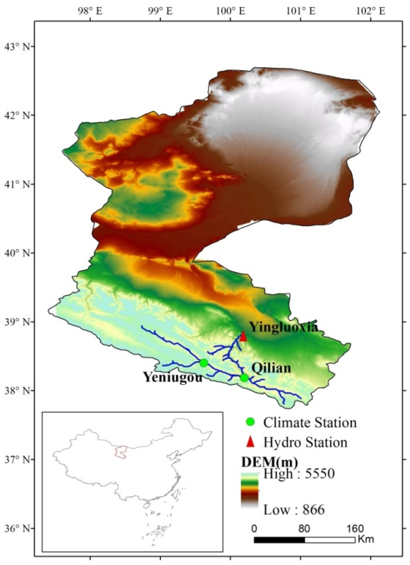
2.1. Study Area
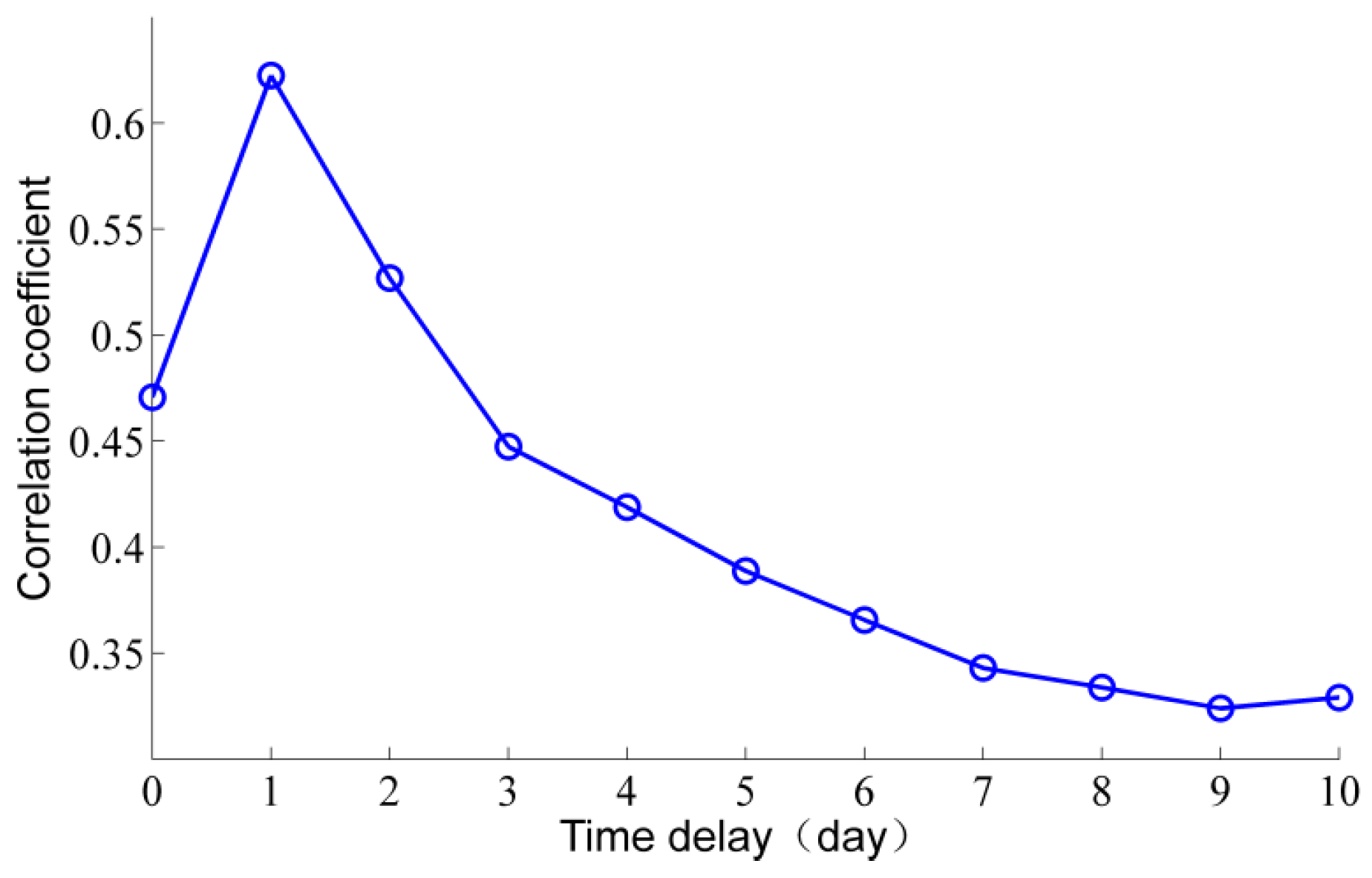
2.2. Precipitation and Streamflow Data
2.3. Discrete Wavelet Transform and Modeling Design
3. Results
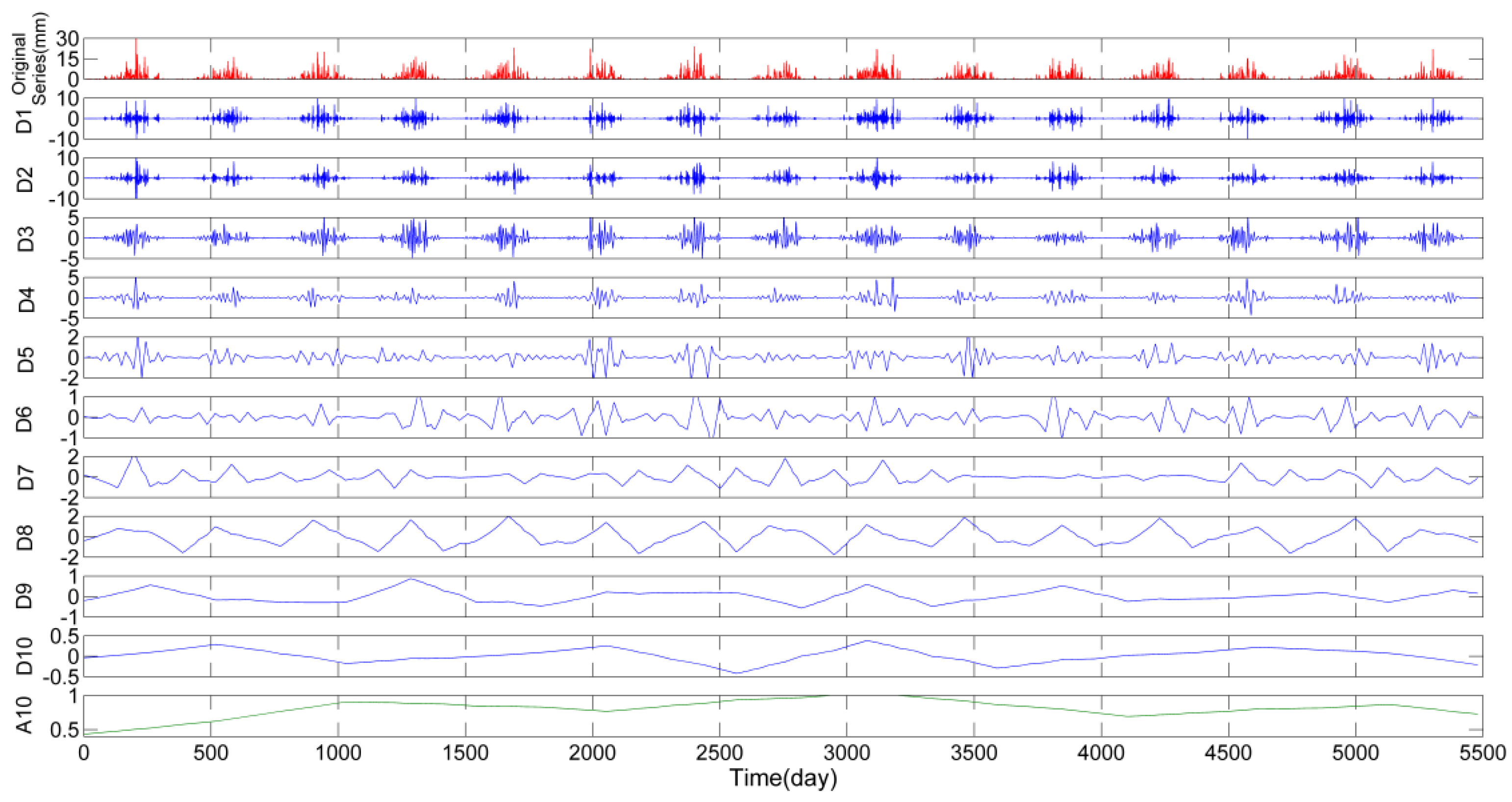
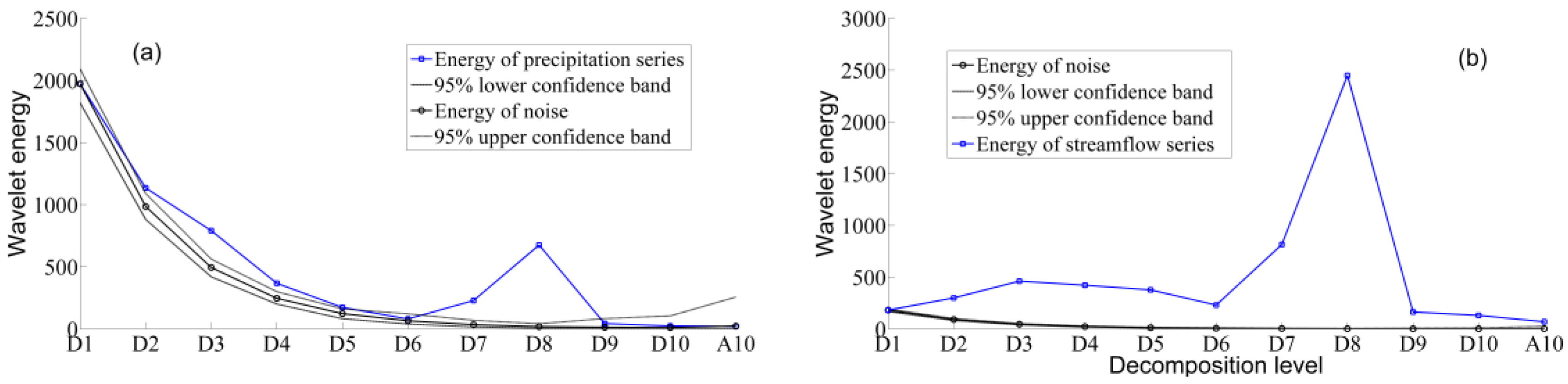
3.1. Wavelet Decomposition of Precipitation
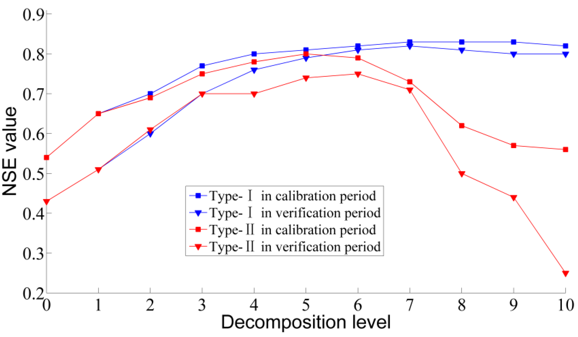
3.2. Forecasting by Different Decomposition Levels
4. Discussion
5. Conclusions
Acknowledgments
Author Contributions
Conflicts of Interest
References
- Cheng, C.T.; Xie, J.X.; Chau, K.W.; Layeghifard, M. A new indirect multi-step-ahead prediction model for a long-term hydrologic prediction. J. Hydrol. 2008, 361, 118–130. [Google Scholar] [CrossRef]
- Tiwari, M.K.; Chatterjee, C. Uncertainty assessment and ensemble flood forecasting using bootstrap based artificial neural networks (banns). J. Hydrol. 2010, 382, 20–33. [Google Scholar] [CrossRef]
- Alvisi, S.; Franchini, M. Fuzzy neural networks for water level and discharge forecasting with uncertainty. Environ. Model. Softw. 2011, 26, 523–537. [Google Scholar] [CrossRef]
- Jain, A.; Kumar, A.M. Hybrid neural network models for hydrological time series forecasting. Appl. Soft. Comput. 2007, 7, 585–592. [Google Scholar] [CrossRef]
- Nourani, V.; Alami, M.T.; Aminfar, M.H. A combined neural-wavelet model for prediction of ligvanchai watershed precipitation. Eng. Appl. Artif. Intel. 2009, 22, 466–472. [Google Scholar] [CrossRef]
- Kisi, O. Wavelet regression model for short-term streamflow forecasting. J. Hydrol. 2010, 389, 344–353. [Google Scholar] [CrossRef]
- Kişi, Ö. Wavelet regression model as an alternative to neural networks for monthly streamflow forecasting. Hydrol. Process. 2009, 23, 3583–3597. [Google Scholar]
- Sang, Y.F. Improved wavelet modeling framework for hydrological time series forecasting. Water Resour. Manag. 2013, 27, 2807–2821. [Google Scholar] [CrossRef]
- Nourani, V.; Baghanam, A.H.; Adamowski, J.; Kisi, O. Applications of hybrid wavelet–artificial intelligence models in hydrology: A review. J. Hydrol. 2014, 514, 358–377. [Google Scholar] [CrossRef]
- Kwon, H.H.; Lall, U.; Khalil, A.F. Stochastic simulation model for nonstationary time series using an autoregressive wavelet decomposition: Applications to rainfall and temperature. Water Resour. Res. 2007, 43. [Google Scholar] [CrossRef]
- Cannas, B.; Fanni, A.; See, L.; Sias, G. Data preprocessing for river flow forecasting using neural networks: Wavelet transforms and data partitioning. Phys. Chem. Earth. 2006, 31, 1164–1171. [Google Scholar] [CrossRef]
- Rajurkar, M.; Kothyari, U.; Chaube, U. Modeling of the daily rainfall-runoff relationship with artificial neural network. J. Hydrol. 2004, 285, 96–113. [Google Scholar] [CrossRef]
- Adamowski, J.; Sun, K. Development of a coupled wavelet transform and neural network method for flow forecasting of non-perennial rivers in semi-arid watersheds. J. Hydrol. 2010, 390, 85–91. [Google Scholar] [CrossRef]
- Grossmann, A.; Morlet, J. Decomposition of hardy functions into square integrable wavelets of constant shape. SIAM J. Math. Ana. 1984, 15, 723–736. [Google Scholar] [CrossRef]
- Maheswaran, R.; Khosa, R. Wavelet–volterra coupled model for monthly stream flow forecasting. J. Hydrol. 2012, 450, 320–335. [Google Scholar] [CrossRef]
- Torrence, C.; Compo, G.P. A practical guide to wavelet analysis. B. Am. Meteorol. Soc. 1998, 79, 61–78. [Google Scholar] [CrossRef]
- Adamowski, J.F. River flow forecasting using wavelet and cross-wavelet transform models. Hydrol. Process. 2008, 22, 4877–4891. [Google Scholar] [CrossRef]
- Kişi, Ö. Neural network and wavelet conjunction model for modelling monthly level fluctuations in Turkey. Hydrol. Process. 2009, 23, 2081–2092. [Google Scholar]
- Nourani, V.; Mogaddam, A.A.; Nadiri, A.O. An ann-based model for spatiotemporal groundwater level forecasting. Hydrol. Process. 2008, 22, 5054–5066. [Google Scholar] [CrossRef]
- Shoaib, M.; Shamseldin, A.Y.; Melville, B.W. Comparative study of different wavelet based neural network models for rainfall-runoff modeling. J. Hydrol. 2014, 515, 47–58. [Google Scholar] [CrossRef]
- Tiwari, M.K.; Chatterjee, C. Development of an accurate and reliable hourly flood forecasting model using wavelet-bootstrap-ANN (WBANN) hybrid approach. J. Hydrol. 2010, 394, 458–470. [Google Scholar] [CrossRef]
- Zhou, H.C.; Peng, Y.; Liang, G.H. The research of monthly discharge predictor-corrector model based on wavelet decomposition. Water Resour. Manag. 2008, 22, 217–227. [Google Scholar] [CrossRef]
- Nourani, V.; Komasi, M.; Mano, A. A multivariate ann-wavelet approach for rainfall-runoff modeling. Water Resour. Manag. 2009, 23, 2877–2894. [Google Scholar] [CrossRef]
- Aussem, A.; Campbell, J.; Murtagh, F. Wavelet-based feature extraction and decomposition strategies for financial forecasting. J. Comput. Intell. Finan. 1998, 6, 5–12. [Google Scholar]
- Partal, T.; Kişi, Ö. Wavelet and neuro-fuzzy conjunction model for precipitation forecasting. J. Hydrol. 2007, 342, 199–212. [Google Scholar] [CrossRef]
- Kisi, O.; Shiri, J. Precipitation forecasting using wavelet-genetic programming and wavelet-neuro-fuzzy conjunction models. Water Resour. Manag. 2011, 25, 3135–3152. [Google Scholar] [CrossRef]
- Shoaib, M.; Shamseldin, A.Y.; Melville, B.W.; Khan, M.M. Hybrid wavelet neuro-fuzzy approach for rainfall-runoff modeling. J. Comput. Civil Eng. 2014, 30, 04014125. [Google Scholar] [CrossRef]
- Shoaib, M.; Shamseldin, A.Y.; Melville, B.W.; Khan, M.M. Runoff forecasting using hybrid Wavelet Gene Expression Programming (WGEP) approach. J. Hydrol. 2015, 527, 326–344. [Google Scholar] [CrossRef]
- Nourani, V.; Kisi, Ö.; Komasi, M. Two hybrid artificial intelligence approaches for modeling rainfall-runoff process. J. Hydrol. 2011, 402, 41–59. [Google Scholar] [CrossRef]
- Li, Z.; Xu, Z.; Shao, Q.; Yang, J. Parameter estimation and uncertainty analysis of swat model in upper reaches of the heihe river basin. Hydrol. Process. 2009, 23, 2744–2753. [Google Scholar] [CrossRef]
- Percival, D.B.; Walden, A.T. Wavelet Methods for Time Series Analysis; Cambridge University Press: Cambridge, UK, 2006. [Google Scholar]
- Daubechies, I. Ten Lectures on Wavelets; Society for industrial and applied Mathematics: Philadelphia, PA, USA, 1992. [Google Scholar]
- Nash, J.E.; Sutcliffe, J.V. River flow forecasting through conceptual models part I—A discussion of principles. J. Hydrol. 1970, 10, 282–290. [Google Scholar] [CrossRef]
- Jain, A.; Srinivasulu, S. Development of effective and efficient rainfall-runoff models using integration of deterministic, real-coded genetic algorithms and artificial neural network techniques. Water Resour. Res. 2004, 40, W04302. [Google Scholar] [CrossRef]
- Sang, Y.F. A practical guide to discrete wavelet decomposition of hydrologic time series. Water Resour. Manag. 2012, 26, 3345–3365. [Google Scholar] [CrossRef]


| Series Type | Period | Statistical Characters | ||||
|---|---|---|---|---|---|---|
| xmean | xmax | xmin | Cv | Cs | ||
| Precipitation (mm) | calibration | 0.85 | 34.70 | 0 | 2.72 | 4.97 |
| verification | 0.84 | 22.00 | 0 | 2.58 | 4.13 | |
| Streamflow (m³/s) | calibration | 50.20 | 788.00 | 5.01 | 1.11 | 3.55 |
| verification | 49.37 | 503.00 | 4.08 | 0.96 | 2.65 | |
| Period | Index | Mode Name * | ||||||||||
|---|---|---|---|---|---|---|---|---|---|---|---|---|
| T-I-0 | T-I-1 | T-I-2 | T-I-3 | T-I-4 | T-I-5 | T-I-6 | T-I-7 | T-I-8 | T-I-9 | T-I-10 | ||
| Calibration | NSE | 0.54 | 0.65 | 0.70 | 0.77 | 0.80 | 0.81 | 0.82 | 0.83 | 0.83 | 0.83 | 0.82 |
| R | 0.74 | 0.81 | 0.84 | 0.88 | 0.89 | 0.91 | 0.91 | 0.91 | 0.91 | 0.91 | 0.91 | |
| AARE | 0.41 | 0.36 | 0.32 | 0.27 | 0.26 | 0.25 | 0.25 | 0.24 | 0.24 | 0.24 | 0.24 | |
| Verification | NSE | 0.43 | 0.51 | 0.60 | 0.70 | 0.76 | 0.79 | 0.81 | 0.82 | 0.81 | 0.80 | 0.80 |
| R | 0.67 | 0.73 | 0.78 | 0.84 | 0.87 | 0.89 | 0.91 | 0.91 | 0.91 | 0.90 | 0.90 | |
| AARE | 0.43 | 0.40 | 0.35 | 0.30 | 0.27 | 0.25 | 0.24 | 0.23 | 0.24 | 0.25 | 0.25 | |
| Period | Index | Mode Name * | ||||||||||
|---|---|---|---|---|---|---|---|---|---|---|---|---|
| T-II-0 | T-II-1 | T-II-2 | T-II-3 | T-II-4 | T-II-5 | T-II-6 | T-II-7 | T-II-8 | T-II-9 | T-II-10 | ||
| Calibration | NSE | 0.54 | 0.65 | 0.69 | 0.75 | 0.78 | 0.80 | 0.79 | 0.73 | 0.62 | 0.57 | 0.56 |
| R | 0.74 | 0.81 | 0.83 | 0.87 | 0.88 | 0.89 | 0.89 | 0.85 | 0.79 | 0.76 | 0.75 | |
| AARE | 0.41 | 0.36 | 0.34 | 0.29 | 0.27 | 0.26 | 0.26 | 0.31 | 0.36 | 0.39 | 0.40 | |
| Verification | NSE | 0.43 | 0.51 | 0.61 | 0.70 | 0.70 | 0.74 | 0.75 | 0.71 | 0.50 | 0.44 | 0.25 |
| R | 0.67 | 0.73 | 0.78 | 0.85 | 0.84 | 0.86 | 0.87 | 0.84 | 0.72 | 0.67 | 0.58 | |
| AARE | 0.43 | 0.40 | 0.35 | 0.29 | 0.31 | 0.28 | 0.29 | 0.32 | 0.39 | 0.45 | 0.40 | |
© 2016 by the authors; licensee MDPI, Basel, Switzerland. This article is an open access article distributed under the terms and conditions of the Creative Commons Attribution (CC-BY) license (http://creativecommons.org/licenses/by/4.0/).
Share and Cite
Yang, M.; Sang, Y.-F.; Liu, C.; Wang, Z. Discussion on the Choice of Decomposition Level for Wavelet Based Hydrological Time Series Modeling. Water 2016, 8, 197. https://doi.org/10.3390/w8050197
Yang M, Sang Y-F, Liu C, Wang Z. Discussion on the Choice of Decomposition Level for Wavelet Based Hydrological Time Series Modeling. Water. 2016; 8(5):197. https://doi.org/10.3390/w8050197
Chicago/Turabian StyleYang, Moyuan, Yan-Fang Sang, Changming Liu, and Zhonggen Wang. 2016. "Discussion on the Choice of Decomposition Level for Wavelet Based Hydrological Time Series Modeling" Water 8, no. 5: 197. https://doi.org/10.3390/w8050197