The Tradeoffs between Market Returns from Agricultural Crops and Non-Market Ecosystem Service Benefits on an Irrigated Agricultural Landscape in the Presence of Groundwater Overdraft

Abstract

Groundwater overdraft has consequences in the long-run for the economic and ecological sustainability of an agricultural landscape. In response to aquifer depletion, we examine the tradeoff of non-market ecosystem service benefits (e.g., groundwater supply, greenhouse gases, and surface water quality) and market returns from crops in the Lower Mississippi River Delta. Farmers may turn to conjunctive water management using on-farm reservoirs and tail water recovery when groundwater pumping becomes expensive. We use separate objectives for market returns from crops and the non-market benefits of ecosystem services to study whether on-farm reservoirs are built with optimal cropping and irrigation choices. The use of reservoirs enables the landscape to attain up to 10% higher market returns for a given level of all non-market ecosystem service benefits by lowering the costs of irrigation, increasing groundwater levels, and reducing fuel combustion and associated greenhouse gas (GHG) emissions from groundwater pumping. A landscape that internalizes both non-market ecosystem service benefits and market value from crops has 30% greater social value than a landscape where only market returns or only non-market value is optimized.

1. Introduction

As the cost of groundwater pumping rises in farming regions, irrigation may rely less on groundwater pumping and more on a coupled use with surface water. This dual use of groundwater and surface water is known as conjunctive water management. Both the economic and institutional aspects of conjunctive water management are well studied [1,2,3], but the influence of irrigation management on the non-market benefits of multiple ecosystem services (in particular, groundwater supply, surface water purification, and greenhouse gas (GHG) reduction) has received less attention. The choice to use conjunctive water management changes the aquifer volume, which in turn affects the crops grown, and the crop production decisions influence nutrient and sediment runoff and GHG emissions. We investigate how conjunctive water management with on-farm reservoirs and tail-water recovery systems influences market returns from crops and non-market ecosystem service values and how this affects the tradeoff between these two objectives on an agricultural landscape.

On-farm reservoirs store surface water abundant in the off-season for later use in the growing season. Tail-water recovery systems bring runoff leaving the agricultural field to a tail-water recovery pit, and this nutrient enriched tail-water from the agricultural field is pumped back to the reservoir for reuse later in the year [4]. There is a suite of non-market ecosystem service benefits that may be affected by the use of the reservoirs and tail-water recovery. Reservoirs may reduce groundwater use and agricultural runoff, but greater rice production may release more methane and destabilize the climate. Although surface water is less expensive to pump than groundwater, there are not necessarily greater economic returns from reservoirs because they occupy productive land and have construction and on-going maintenance costs.

The Lower Mississippi River Basin in Arkansas (a farming region referred to as the Arkansas Delta) has long relied on groundwater from the Mississippi River Valley Alluvial Aquifer. The supplies of groundwater will fall short of agricultural demand for groundwater in 2050 by 7 million acre-feet per year [5]. We use a dynamic spatially explicit farm landscape to optimize farm net returns and ecosystem services by changing the extensive crop margin, the shift in crops such as rice that are irrigation intensive to crops like wheat that are not irrigated, and the irrigation water source, either reservoir or well. Reducing the irrigation water applied to the crop in response to groundwater scarcity through deficit irrigation does not appear to be a common in practice over the long run, which is the time frame relevant for considering groundwater depletion [6]. The presence of reservoirs with tail-water recovery systems to supplement the groundwater is likely to rise with groundwater pumping costs.

The non-market benefits of groundwater supply, surface water purification, and GHG emissions change in response to farm production decisions at the landscape scale. The aquifer’s saturated thickness, hydro-conductivity, and the proximity to nearby wells affect groundwater flows. The slope of the land and the tillage and irrigation practices affect soil and phosphorous runoff that can reduce the quality of waterbodies. Farm practices, soil type, and fuel combustion from irrigation pumping all influence release of GHGs. To compare non-market ecosystem service values and market value from agricultural crops, we use estimates of non-market values from the scientific literature for the ecosystem services to put them in monetary terms.

An efficiency frontier for the landscape is made by maximizing the market returns over the feasible range of non-market ecosystem service values. The tradeoff of least ecosystem service value foregone to achieve greater economic return is observed as the slope of the frontier. The landscape that is societally optimal is where the loss of a dollar of non-market ecosystem service value is exactly balanced by a dollar gain in market returns (Figure 1). Elsewhere on the frontier, a movement along the frontier increases social value by rebalancing toward the objective that gives more value than is given up.

When there is the building of on-farm reservoirs with tail-water recovery on the landscape, the efficiency of the landscape at providing market and non-market value can rise, and this would mean the frontier shifts outward. Since planners may look at only one non-market ecosystem service value, a frontier comparing only one ecosystem service value to economic returns can reveal whether investment in reservoirs and tail-water recovery systems are worthwhile in every case and how the other ecosystem services fare. The crop and water choices when only groundwater value is considered may suggest that reservoir and tail-water recovery systems are a great investment, but when all the ecosystem services are taken into account, the additional release of GHGs make reservoirs only look like a marginal social investment.

Earlier papers looking at ecosystem services and economic returns from an agricultural landscape with groundwater depletion driving landscape change do not consider the spatially explicit tradeoff among economic returns and carbon sequestration [4,7]. Prior work considers tradeoffs among multiple environmental objectives or economic returns [8,9,10,11,12]. These studies find that bundles of land use generate different services such as intensive agricultural production being associated with high production of agricultural products but low water quality and carbon storage. A branch of this research uses efficiency frontiers, which are able to analyze the optimal tradeoffs among ecosystem services or economic returns. The tradeoff between carbon sequestration and species conservation use but not economic returns, and the tradeoff between species conservation but not ecosystem services and economic returns has been considered [13,14]. Marine spatial planning that considers multiple ecosystem services is informed by efficiency frontiers [15]. This earlier work with efficiency frontier does not look at the tradeoffs between economic returns and groundwater, water quality, and greenhouse gas sequestration value or consider the influence of an irrigation practices such as conjunctive water management.

2. Method

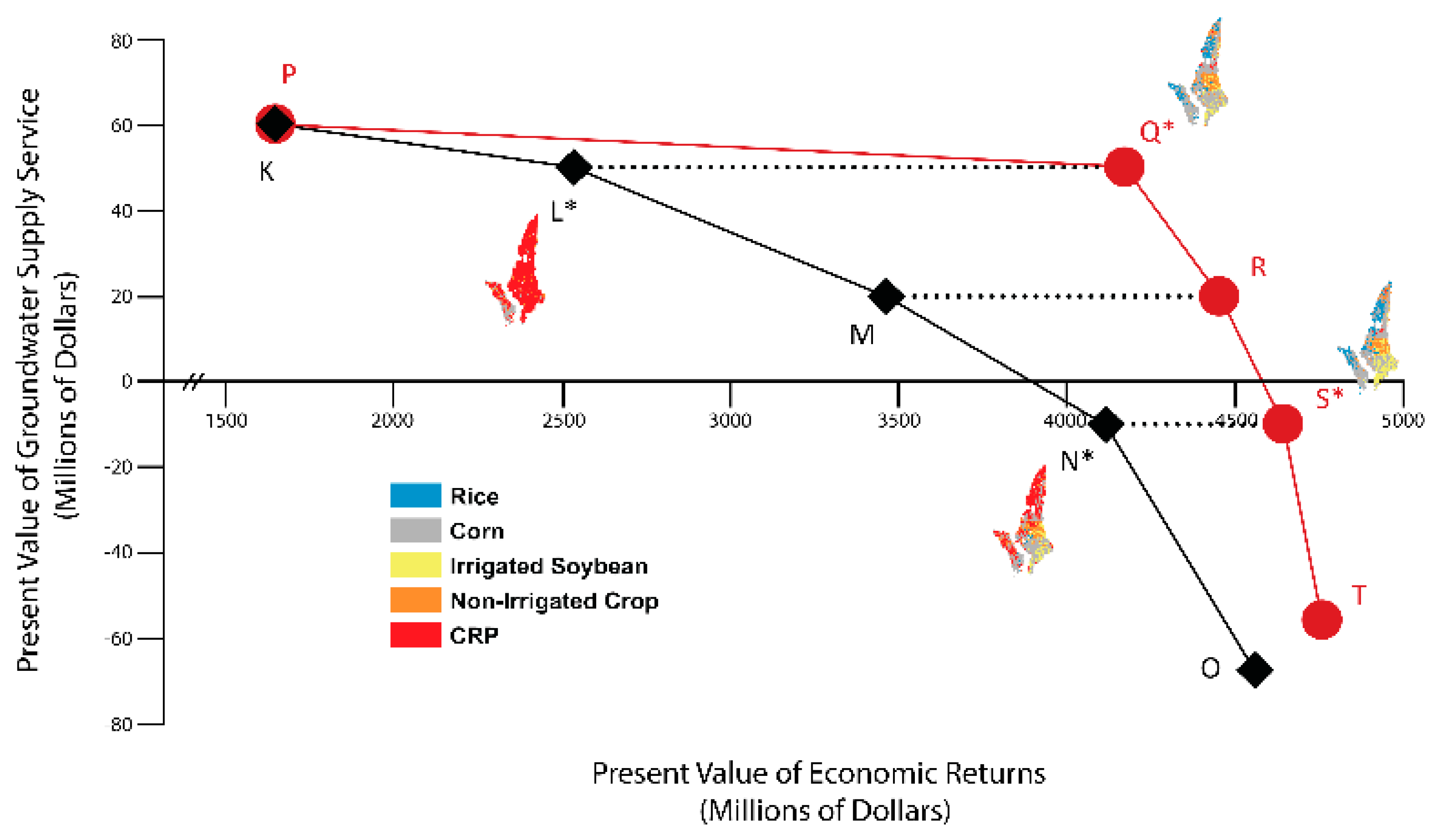
The land cover of the farm landscape includes crops, reservoirs, and conserved land set aside through a rental program of the government. The chosen crops generate economic returns, but irrigation depletes groundwater. Also, agricultural runoff pollutes surface water, and farm production activities release GHGs. The landscape is spatially heterogeneous due to differences in long term investment in farm practices, soil types, and access to water resources. A time horizon T is chosen for a single generation of farmers to observe how depletion of the aquifer influences production decision, and a grid of m cells (sites) represents spatial differences.

The major crops include irrigated rice, soybean, corn, and cotton, non-irrigated sorghum and soybean, and double cropped irrigated soybean with winter wheat. There are n possible land cover types j at the end of period t as denoted by L_ijt for site i that include each of the crops, reservoirs that have tail-water recovery, and the US Department of Agriculture’s Conservation Reserve Program (CRP). At the end of each annual period t, we assume any other land cover j can become on-farm reservoirs and tail-water recovery or CRP, and after a ten-year period CRP can transition into a crop. A profit maximizing farmers may switch land out of irrigated crops into non-irrigated crops with declining groundwater availability at the end of each period.

The initial land availability equals the sum of the land covers chosen for site i at any time t (Equation (1)).

$${\displaystyle {\sum }_j^n{L}_{ijt}}={\displaystyle {\sum }_j^n{L}_{ij0}}$$

(1)

where j = crops, CRP, on-farm reservoirs.

2.1. The Economic Model

The net present value of the agricultural production over all time periods and the entire landscape is the economic objective. The average annual irrigation that crop j receives to supplement precipitation, wd_j, is the demand for irrigation in acre-feet. The groundwater stored in the aquifer beneath site i at the end of the period t is AQ_it. The water that comes from the on-farm reservoirs is RW_it, and the water from well-pumping is GW_it. There is recharge of the groundwater, nr_i, that occurs naturally from precipitation, streams, and underlying aquifers each period.

Equation (2) shows the acre-feet of water stored in an acre reservoir as

$$\left({\omega }_{\text{max}}+{\omega }_{\text{min}}\right)-\frac{{\omega }_{\text{max}}}{{\displaystyle {\sum }_j^n{L}_{ij0}}}{L}_{iRt}$$

(2)

which includes, $L_{iRt}$, as the acres in reservoirs at time t, and the total acreage at site i, ${\sum }_j^n{L}_{ij0}$ [7]. If the reservoir occupies the entire site i and only the rainfall fills the reservoir, then the low-end acre-feet of water that fills each reservoir acres is ${\omega }_{\text{min}}$. If the reservoir is less than the size of the site, then recovery of the runoff and rainfall fills the reservoir to a high-end capacity in acre-feet per reservoir acre of $\left({\omega }_{\text{max}}+{\omega }_{\text{min}}\right)$. We do not account for annual variability in the evaporation, leakage, and the timing of rainfall within a growing season, which could influence ${\omega }_{\text{max}}$ and ${\omega }_{\text{min}}$ for the reservoir. The use of reservoirs and tail-water recovery systems reduces water that reaches streams, and this limits the water available to downstream users and the environment during the growing season. However, most of the water used from the reservoirs is collected in the rainy season before planting.

The intensity of well-pumping across the landscape influences the way in which aquifer depletion varies over space. The proportion of the underground flow into the aquifer at site k and out of site i when an acre-foot is pumped from a well at site k is p_ik, which depends on the distance and the lateral speed of underground water movement based on the soil profiles observed between sites [2]. This means the groundwater that leaves site i is ${\sum }_k^m{p}_{ik}G{W}_{kt}$. We assume pumps have the same efficiency and power units to deliver a fixed amount of water per minute.

The water used for irrigation must be less than the water available from reservoirs and wells (Equation (3)), and Equation (4) indicates that the water stored in the reservoirs must be greater the water used from the reservoirs. The aquifer volume in the previous period less the spatially weighted proportion of water pumped from the surrounding sites plus natural recharge equals the current aquifer volume (Equation (5)). The cost of pumping groundwater at a site, GC_it, depends on the cost to lift an acre-foot of water by one foot, c^p, and the initial depth to the groundwater, dp_i. The depletion of the aquifer volume, $\left(A{Q}_{i0}-A{Q}_{it}\right)$, divided by the area of the site, ${\sum }_j^n{L}_{ij0}$, shows how much the depth to the aquifer increases. Capital costs per acre-foot for the well, which accounts for new well-drilling in response to aquifer decline, is c^c (Equation (6)).

$${\displaystyle {\sum }_{j=1}^{n}w{d}_j{L}_{ijt}}\le G{W}_{it}+R{W}_{it}$$

(3)

$$R{W}_{it}\le \left(\left({\omega }_{\text{max}}+{\omega }_{\text{min}}\right)-\frac{{\omega }_{\text{max}}}{{\displaystyle {\sum }_j^n{L}_{ij0}}}{L}_{iRt}\right)L_{iRt}$$

(4)

$$A{Q}_{it}=A{Q}_{i(t-1)}-{\displaystyle {\sum }_k^m{p}_{ik}G{W}_{kt}}+n{r}_i$$

(5)

$$G{C}_{it}=c^c+c^p\left(d{p}_i+\frac{\left(A{Q}_{i0}-A{Q}_{it}\right)}{{\displaystyle {\sum }_j^n{L}_{ij0}}}\right)$$

(6)

The cost to produce an acre of the crop excluding the irrigations costs ca_j and the price per conventional unit of the crop is pr_j are constant in real terms. We assume no productivity growth trend for the constant yield of crop j per acre at site i, y_ij. Excluding the costs of irrigation, the net value for crop j is then pr_jy_ij − ca_j per acre. The CRP payment per acre to the landowner, pr_crpy_icrp, with yield normalized to one and price is the payment per acre, less the cost to establish and maintain an acre of CRP (ca_crp) is net value per acre of CRP. The reservoir pumping cost per acre-foot is c^rw, and the per acre capital and maintenance cost of a reservoir each period is c^r. We make values over time comparable in monetary terms using the real discount factor, ${\delta }_t$.

Equation (7) indicates the economic objective to maximize the present value of farm profits over the fixed horizon T by changing the amount of land in each crop or CRP, the reservoir water use, and groundwater use, namely L_ijt, RW_it, and GW_it. The initial condition of the state variables and the non-negativity constraints on land, water use, and the aquifer are shown in Equations (8) and (9).

$$\underset{L_{ijt},R{W}_{it},G{W}_{it}}{\text{max}}:{\displaystyle \sum _{t=1}^T{\delta }_t\left({\displaystyle \sum _{i=1}^m{\displaystyle \sum _{j=1}^n\left(p{r}_j{y}_{ij}-c{a}_j\right)L_{ijt}-c^r{L}_{iRt}-c^{rw}R{W}_{it}-G{C}_{it}G{W}_{it}}}\right)}$$

(7)

Subject to:

$$L_{ij0}=L_0^{ij},L_{iR0}=0,A{Q}_{i0}=A{Q}_0^i,$$

(8)

$$L_{ijt}\ge 0,R{W}_{it}\ge 0,G{W}_{it}\ge 0,A{Q}_{it}\ge 0$$

(9)

and the spatial dynamics of land and irrigation (Equations (1)–(6)). The crop and irrigation choices from the optimization of Equation (7) influence ecosystem services related to GHGs, water purification, and groundwater availability, but they are not directly considered by producers.

2.2. The Ecosystem Service Model

We track changes in the physical ecosystem services over time and use estimates of non-market values taken from the scientific literature to determine the monetary value of the changes in ecosystem services to calculate the net present value of ecosystem services from the landscape.

GHG emissions per acre of vegetation on a land cover are associated with the production of crops and CRP for the major production practices of the Arkansas Delta based on a life cycle assessment (LCA) up to the farm gate [16]. Fuel use and emissions generated during the manufacture of chemicals and fertilizer, methane emissions from rice production, and nitrous oxide emissions from the application of nitrogen fertilizer to soil are tracked in carbon equivalents (CE) in kg per acre for land cover j ($E_j$). Pumping ground and reservoir water releases fuel combustion emissions, and the range of irrigation emissions is shown in Figure S1. The depth of the well multiplied by a conversion factor ${\sigma }_g$ that identifies the carbon emitted from fuel combustion to lift an acre-foot of water one foot and multiplied by the acre-feet of groundwater pumped indicate the emissions from groundwater pumping at site i, $E{G}_{it}$. The acre-feet of reservoir water pumped multiplied by a conversion factor ${\sigma }_r$ for the carbon emitted from fuel combustion to pump an acre-foot of water into a reservoir and back out to the field is the emissions from pumping reservoir water at site i, $E{R}_{it}$. The total carbon emissions for time t at site i ($E_{it}$) is shown in Equation (10) as

$$E_{it}={\displaystyle {\sum }_j^n{E}_j}{L}_{ijt}+E{G}_{it}+E{R}_{it}$$

(10)

Aboveground biomass ($AG{B}_{ij}$) and belowground biomass ($BG{B}_{ij}$) sequester carbon, with the parameter values in the Supplementary Materials, and this sequestration depends on the soil texture and tillage practices [17]. A weighting of soil textures at each site i determines the soil factor, ${\xi }_i$, which is the fraction of carbon lost to respiration due to soil related microbial activity. Porous soil (i.e., sandy) has more intense wetting and drying cycles, and this encourages microbial activity and respiration compared to finer textured soils (i.e., clay). Equation (11) tracks the carbon sequestration, $S_{it}$, for time t at site i as

$$S_{it}={\displaystyle {\sum }_j^n\left[\left(AG{B}_{ij}+BG{B}_{ij}\right){\xi }_i\right]}{L}_{ijt}$$

(11)

Although the sequestration is likely to be greater initially and slower later on CRP land, we suppose sequestration occurs evenly over time [18]. Equations (10) and (11) constrain the ecosystem services objective but do not influence the economic returns objective.

The cost to society incurred by the predicted damages from each additional ton of carbon equivalent emitted to the atmosphere is the social cost of carbon, $p_c$, and this indicates the monetary value of a ton less of carbon equivalent GHGs from the agricultural landscape [19]. Equation (12) says the value of avoided damages, $V_c$, is negative if the emissions outweigh sequestration (Equation (12)).

$$V_c={\displaystyle \sum _{t=1}^T{\delta }_t}\left({\displaystyle {\sum }_i^m{p}_c\left(S_{it}-E_{it}\right)}\right)$$

(12)

We use the InVEST (Integrated Valuation of Ecosystem Services and Tradeoffs) water purification model to estimate how sediment, phosphorus, and nitrogen runoff responds to land cover transitions [20]. Natural land, urban areas, public land, and lakes are in the water purification model, although not part of the land cover in the optimization model, because they affect the agricultural runoff from each site that reaches streams. Based on soil characteristics, precipitation, slope, and evapotranspiration, the expected annual water yield at each site is calculated. The expected pollutant loading and the filtering capacities for each land cover is combined with the water yield to calculate the pollutants from each site that eventually reach a stream. The initial land cover determines pollutant k export per acre from land cover j for farm site i reaching a stream, $P_{ijk0}$. We assume pollutant exports from site i are associated only with the land cover changes at site i but not the land cover changes at surrounding sites. Tail-water recovery systems with reservoirs capture runoff, and the slope at site i affects the effectiveness of the system. The tail-water recovery system effectiveness, $0\le {\theta }_i\le 1$, is greater if site i is flatter [21].

Equation (13) indicates the amount of pollutant k reaching the mouth of a watershed from each site i at time t ($E{X}_{ikt}$) as

$$E{X}_{ikt}={\displaystyle {\sum }_j^n{P}_{ijk0}{L}_{ijt}}\left(1-{\theta }_i\frac{L_{iRt}}{\left(L_{iRt}+1\right)}\right)$$

(13)

where $P_{ijk0}{L}_{ijt}$ is the export without reservoirs of the pollutant k to a stream from site i and land cover j [7]. A site with reservoirs has a value less than one for ${\theta }_i\frac{L_{iR\_t}}{\left(L_{iR\_t}+1\right)}$ because there is land in $L_{iR\_t}$, and this reduces the export of pollutants to streams.

The willingness to pay (WTP) per household for a water purification improvement ($wtp{q}_b$) depends on the baseline water quality and median household income of the basin b. The WTP values per household are prorated to the percent reduction in the pollutant k loading from all sites i in basin b, $\left(\frac{{\displaystyle \sum _{i\in b}\left(E{X}_{ikt}-E{X}_{ik(t+1)}\right)}}{{\displaystyle \sum _{i\in b}E{X}_{ikt}}}\right)$. We use ${\displaystyle \sum _{i\in b}\left(E{X}_{ikt}-E{X}_{ik(t+1)}\right)}$ because a fall in pollutant exports corresponds to an increase in water purification value. Multiplying the number of households in the basin ($h{h}_b$) by the prorated WTP per household for pollutant k is the present value of the surface water purification, $V_w$, shown as Equation (14)

$$V_w={\displaystyle \sum _{t=1}^T{\delta }_t}\left({\displaystyle \sum _k{\displaystyle \sum _{b}h{h}_{b}wtp{q}_b\left(\frac{{\displaystyle \sum _{i\in b}\left(E{X}_{ikt}-E{X}_{ik(t+1)}\right)}}{{\displaystyle \sum _{i\in b}E{X}_{ikt}}}\right)}}\right)$$

(14)

We consider only the groundwater value to agricultural producers to buffer against periodic shortages in surface water supplies, $p_{bv}$, because there is inadequate data to estimate the damages from subsidence and losses to in-stream flows. Aquifer volume falls if the natural recharge of the aquifer is less than the groundwater withdrawal for irrigation. Equation (15) indicates the present value of the groundwater buffer value, $V_g$, as

$$V_g={\displaystyle \sum _{t=1}^T{\delta }_t}\left({\displaystyle {\sum }_i^m{p}_{bv}\left(A{Q}_{i(t+1)}-A{Q}_{it}\right)}\right)$$

(15)

The sum of the present value of GHG reduction, surface water purification, and groundwater buffer value is the ecosystem services objective (Equation (16)). The objective is to maximize the present value of ecosystem services by determining L_ijt, RW_it, and GW_it over the fixed time horizon T

$$\underset{L_{ijt},R{W}_{it},G{W}_{it}}{\text{max}}:V_c+V_w+V_g$$

(16)

subject to the Equations (1)–(6), (10), (11) and (13). The crop and irrigation choices from the optimization of Equation (16) influence farm profits but they are not directly considered by planners.

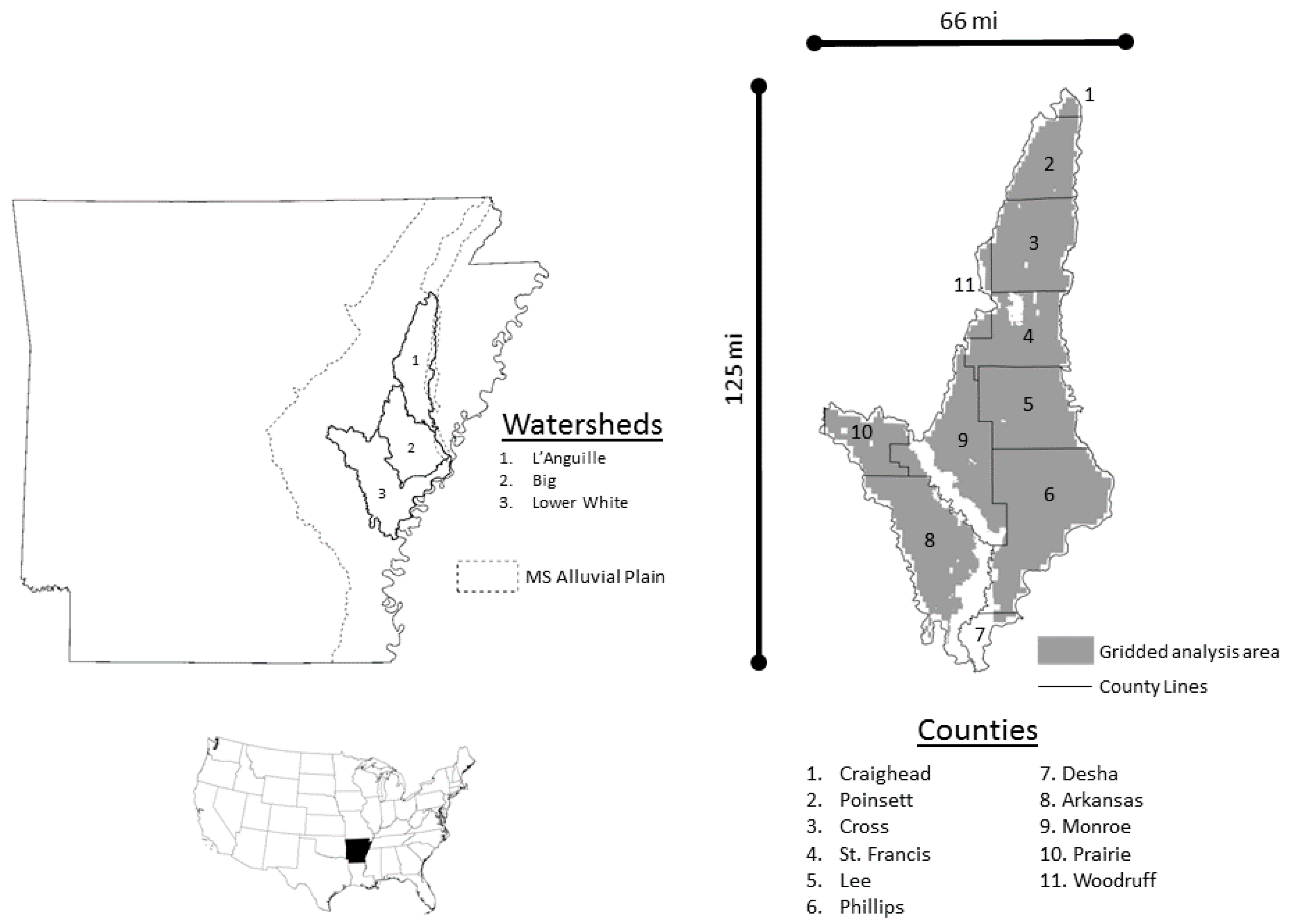
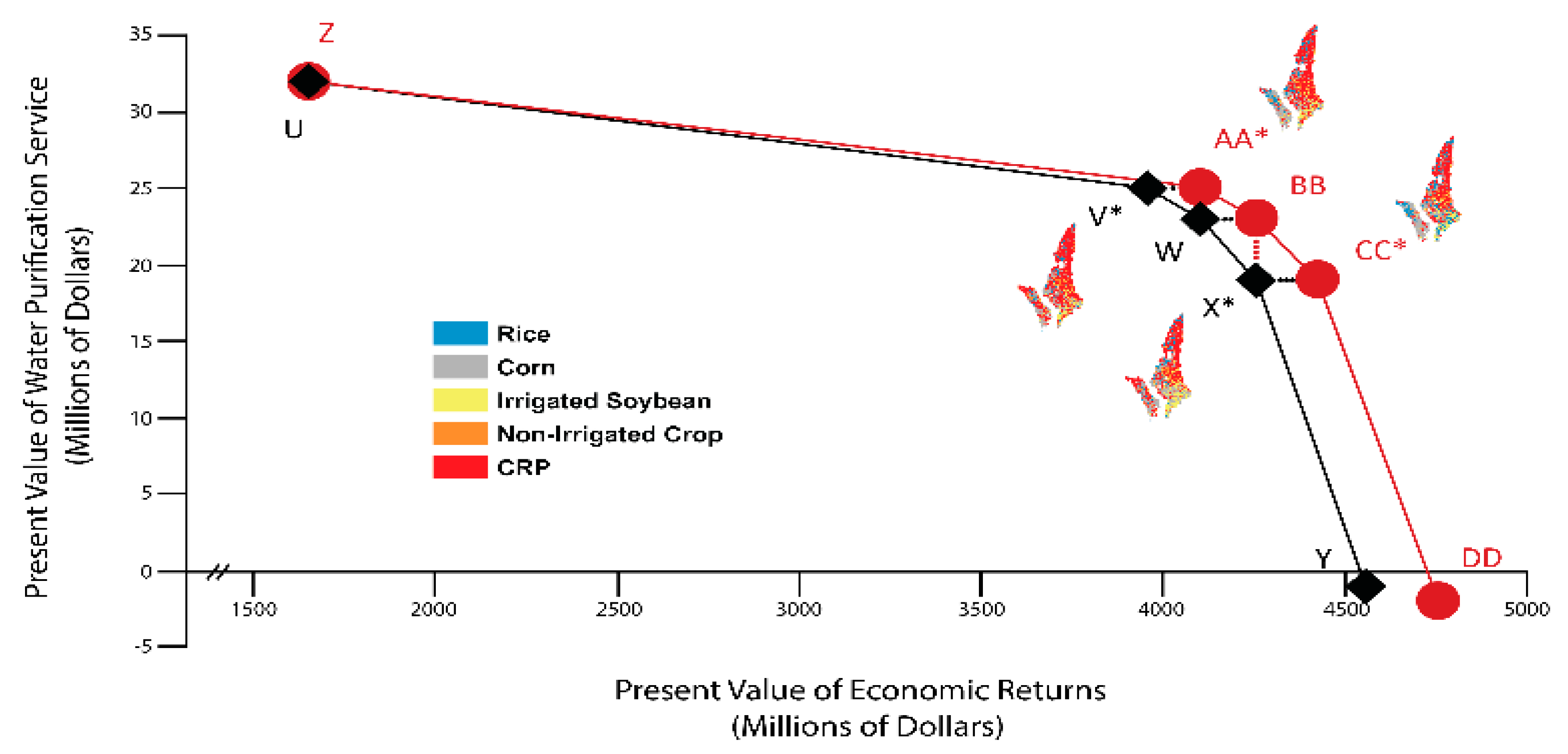
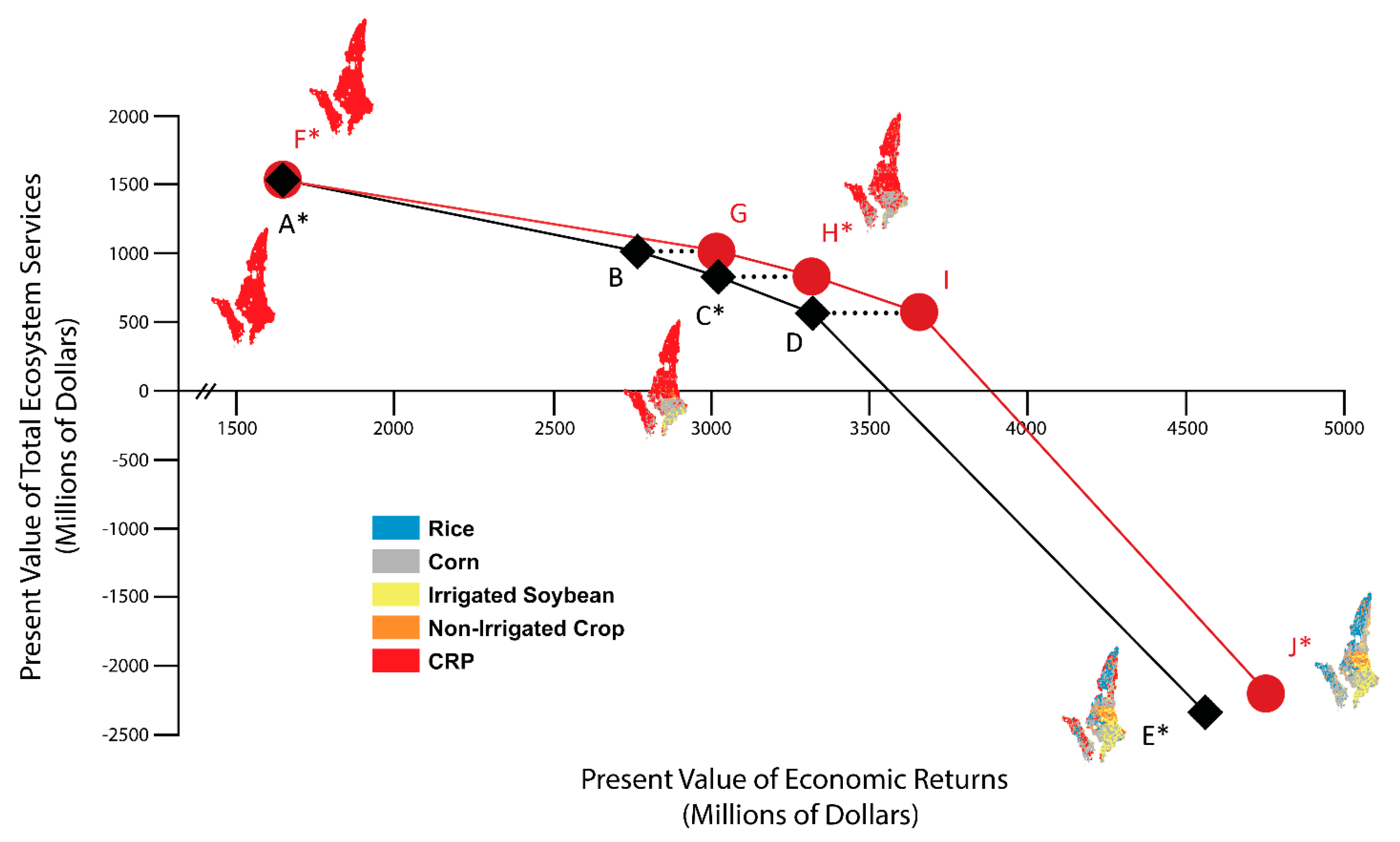
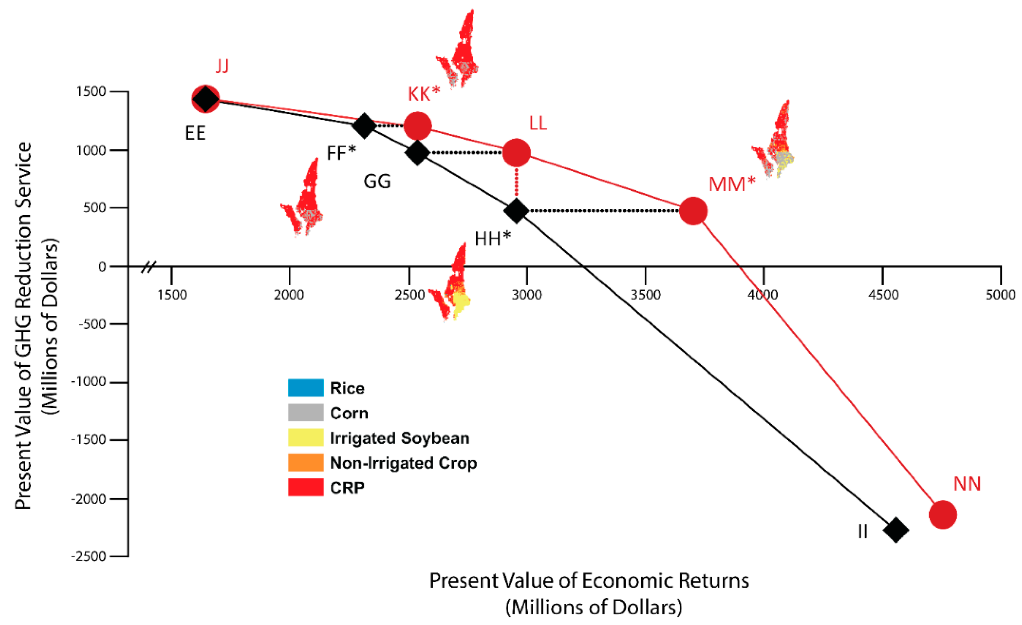
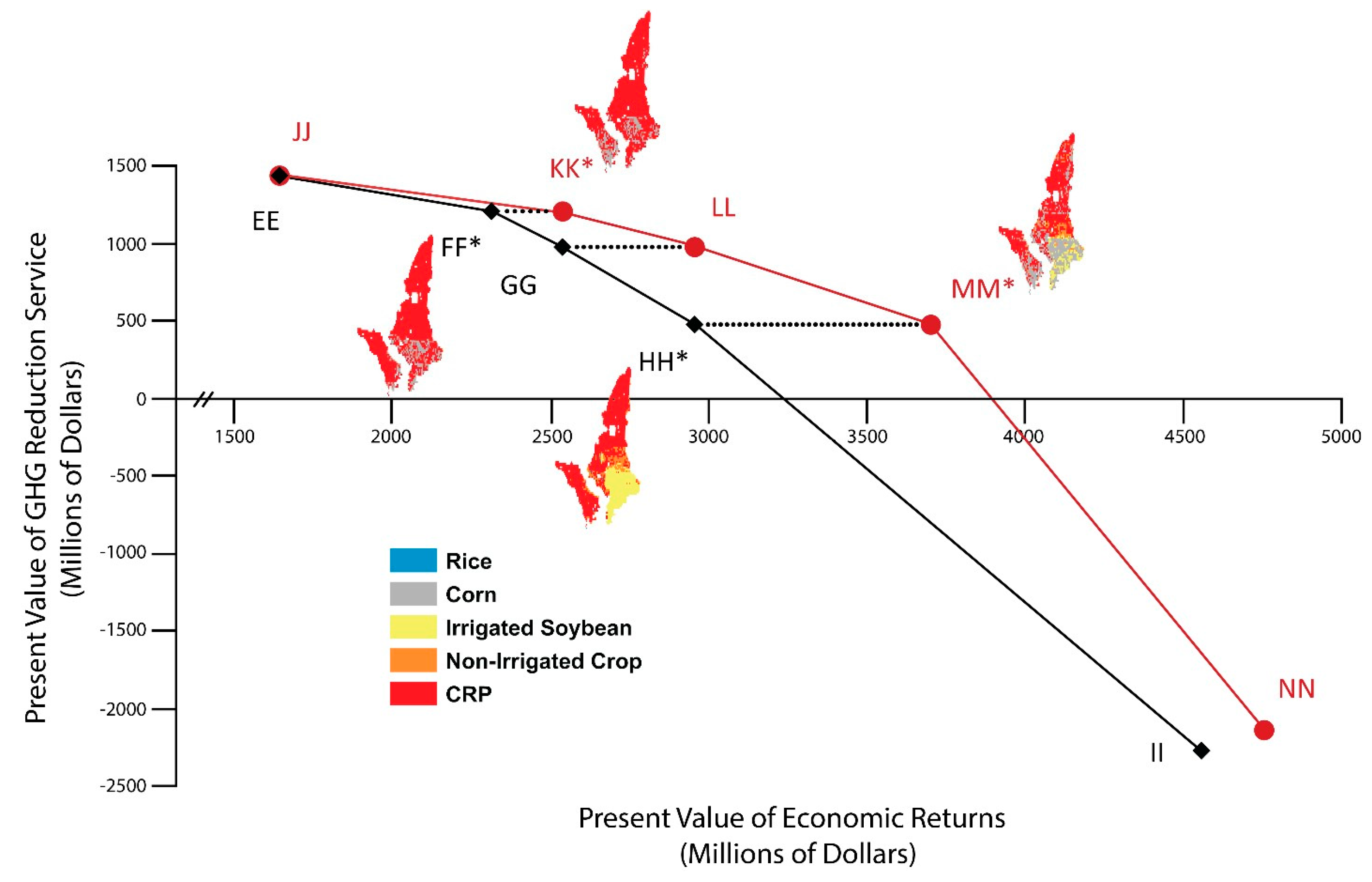
2.3. Efficiency Frontier

We trace out an efficiency frontier, showing the tradeoff of non-market ecosystem service value and market economic returns, by finding the maximum economic returns for a fixed value of an ecosystem service, and then varying the fixed non-market value of the ecosystem service over its entire potential range [13,14]. We compare how the reservoirs affect the shape and position of the efficiency frontier by finding efficiency frontiers without and with reservoirs. The efficiency frontier illustrates the greatest market return and non-market values feasible on the landscape and the necessary reduction in non-market value to increase market returns from the landscape.

By optimizing the non-market ecosystem service benefit objective without a restriction on market returns, the maximum non-market value of the ecosystem services is found. Conversely, by optimizing market returns without restriction on the ecosystem service value, the minimum non-market value of the ecosystem services is found. Next, ecosystem service values are chosen that extend for the range of minimum and the maximum ecosystem service values to trace out the shape of the frontier. Lastly, for each level of ecosystem service value from the previous step, we maximize market returns. A combination that rests on the efficiency frontier is a market returns maximum that corresponds to a given non-market ecosystem service value.

Non-market ecosystem service benefits for the efficiency frontier with reservoirs are chosen because they match the non-market ecosystem service values chosen for the efficiency frontier without reservoirs. A determination of the gains from moving to an outer frontier is possible by using the same non-market ecosystem service values across frontiers. We trace out the rest of the frontier with reservoirs by choosing evenly spaced ecosystem service values. We use the non-linear programming solver CONOPT from AKRI Consulting and Development to perform the optimization in the Generalized Algebraic Modeling System (GAMS) [22].

2.4. Conservation Policies

Conservation policies aim to align profit-making decisions with the provision of non-market ecosystem service value. We compare the model of the market returns objective with reservoirs and no conservation policy to the conservation policies that include cost-share on reservoir construction costs, tax on groundwater use, a total maximum daily load of phosphorous and sediment, and carbon credits. The policies for the cost-share on reservoir costs and groundwater taxes result in transfers between the government and producers while the carbon credits cause transfers among producers. A conservation policy should increase the total value to society, which is the economic returns less transfers from the government plus the ecosystem service value.

3. Data

The outer boudary of the study area consists of three eight-digit hydrologic unit code watersheds in the Arkansas Delta region with critical groundwater areas and non-point source pollution priorities (Figure 2). These watersheds overlap eleven Arkansas counties, and the average for the past 5 years of crop yields by county is a proxy for the yield of the crops [23]. We evaluate crop mix and irrigation methods on a landscape with spatial heterogeneity by dividing the study area into 2724 sites. Sites having entirely non-cropland uses, e.g., public lands water, and urban areas, in the 2013 Cropland Data Layer (CDL) are removed [24]. The initial acreage of rice, corn, cotton, soybeans, and sorghum comes from the 2013 CDL, and on the basis of harvested acreage for 2010–2011 the soybean acreage is split into non-irrigated soybean, irrigated soybean, and double crop soybeans (Table S1) [25]. The yield of the 30-year Treasury Bond over the last decade suggests a real discount rate of 5% [26].

3.1. Aquifer

Table S1 shows the initial depth to the water table and saturated thickness of the Alluvial aquifer from the Arkansas Natural Resources Commission [27]. The acreage of the site times the saturated thickness of the aquifer is the volume of the aquifer at site i. Precipitation and the flow from streams and the underlying Sparta aquifer influences the natural recharge (nr_i) [28]. The spatial weight (p_ik) based on soil properties and proximity determines how well-pumping reduces the aquifer beneath the surrounding cells [2]. The data for the aquifer model are shown in more detail above in Table S1. Based on the variability of seasonal rainfall, the curvature of the soybean yield response to water, and net profit of soybeans, the constant in real terms estimate of the per-acre-foot groundwater is $5.19 [2].

3.2. Farm Production and the On-Farm Reservoir and Tail-Water Recovery System

The costs of production by crop from the 2014 Crop Cost of Production estimates, excluding irrigation, are shown in Table S2 [29]. The crop specific irrigation water use comes from the Division of Agriculture [22]. The five-year average of December futures prices for harvest time contracts for all crops are used for the crop prices [30]. The sign-ups in Arkansas as of March 2015 indicate the CRP payment per acre [31].

The minimum volume of water (ω_min) an acre reservoir will hold comes from the tail-water recovery system collecting rainfall alone to fill a reservoir by 1.4 acre-feet of water [32]. The maximum capacity accounting for evaporation of 11 acre-feet per acre is based on irrigation runoff supplementing the rainfall runoff [33]. The average share of nutrients and sediment captured by reservoirs (${\theta }_i$) varies according to the slope of each site i, and this is about 0.87 [4,34].

3.3. Water Purification and Greenhouse Gases

A digital elevation model directs surface water downhill in a geographic information system (GIS). As the water travels over each site, the site either subtracts of adds, depending on the land cover, to the quantity of the nutrient (Table S3) and sediment (Table S4) that reaches a stream. The cumulative loadings to the mouth of a watershed is the export of the nutrients and sediment from all the sites in the watershed that reach the streams.

In a contingent valuation study of agricultural nonpoint pollution in Mississippi, Hite et al. find an average willingness to pay (WTP) value per household per year of $49.94 for a 20% reduction in pollutant loadings and $46.97 for a 10% reduction in pollutant loadings [35]. The more conservative estimate of WTP to pay used for the analysis is based on the 20% reduction in pollutant loadings. The multiplication of the household WTP prorated to the percentage reduction in loadings at the mouth of each watershed and the projected number of households in the basin gives the WTP per basin in each period [36].

Using the production estimates from crop enterprise budgets, we track greenhouse gas emissions from fuel, fertilizer, and chemical applications [28]. We track above and below ground biomass production with county level yields to determine soil carbon sequestration [17]. Plant residue left in the soils becomes a fraction of carbon after microbial decomposition and gas fluxes (Table S5). Further adjustment to carbon sequestration occurs based on tillage and soil texture. Emissions from irrigation fuel combustion change in response to the model outcome for the depth to the aquifer.

There is social value to reduction of GHGs in the atmosphere because of avoided damages from climate change. Based on the fitted median distribution and a 1% pure rate of time preference from and after adjusting to 2013 dollars, the constant real estimate is $129 per ton carbon equivalent ($35.14 per ton CO₂e) [19]. The social value to reduce GHGs is much higher than the prices for carbon created by governmental bodies throughout the world, where the majority of emissions have prices less than $10 per ton CO₂e [37].

4. Results

Four sets of efficiency frontiers (shown in Figure 3, Figure 4, Figure 5 and Figure 6) examine the tradeoff of non-market ecosystem service benefits necessary to increase market economic returns. A set of efficiency frontiers includes one without on-farm reservoirs and one with on-farm reservoirs. The tradeoff differs depending on whether the model includes all the ecosystem services (Points A to J), groundwater supply value only (Points K to T), water purification value only (Points U to DD), or GHG reduction value only (Points EE to NN).

Point A in Figure 3, where all the land is put into CRP, generates the maximum value of non-market ecosystem services when all ecosystem service benefits are taken into account. The rental payments by the government for CRP mean the landscape at Point A also has positive economic returns. Moving from point A to point C increases economic returns by 83% while reducing the non-market value of all ecosystem services by 47% (see

Table 1. Ecosystem service and economic return values for points along efficiency frontiers.

Without Reservoirs				With Reservoirs
Efficiency Frontiers	Present Value of Economic Returns	Present Value of Optimized Ecosystem Service(s)	Present Value of Ecosystem Services	Efficiency Frontiers	Present Value of Economic Returns	Present Value of Optimized Ecosystem Service(s)	Present Value of Ecosystem Services
All ecosystem service values
A	1,649	1,532	1,532	F	1,649	1,532	1,532
B	2,768	1,000	1,000	G	3,021	1,000	1,000
C	3,021	819	819	H	3,322	819	819
D	3,322	567	567	I	3,656	567	567
E	4,559	−2,345	−2,345	J	4,757	−2,206	−2,206
Groundwater supply values only
K	1,649	60	1,532	P	1,650	60	1,529
L	2,539	50	885	Q	4,169	50	−620
M	3,463	20	331	R	4,449	20	−796
N	4,118	−10	−450	S	4,638	−10	−1,178
O	4,559	−68	−2,345	T	4,757	−56	−2,206
Water purification values only
U	1,649	32	1,532	Z	1,649	32	1,531
V	3,957	25	−1,526	AA	4,102	25	−1,348
W	4,102	23	−1,699	BB	4,260	23	−1,524
X	4,260	19	−1,895	CC	4,429	19	−1,720
Y	4,559	−1	−2,345	DD	4,757	−2	−2,206
Greenhouse gas reduction values only
EE	1,649	1,439	1,532	JJ	1,649	1,439	1,532
FF	2,319	1,200	1,269	KK	2,456	1,200	1,276
GG	2,456	9,69	1,033	LL	2,961	969	1,033
HH	2,961	478	516	MM	3,708	478	5,18
II	4,559	−2,276	−2,345	NN	4,757	−2,147	−2,206

Note: The values of economic returns and ecosystem service values are reported in millions of 2013 constant dollars.

). The switch from CRP to irrigated corn and non-irrigated crops raises market returns (see

Table 2. Present value of economic returns and ecosystem services for select points on the efficiency frontier using all ecosystem service value (in millions of 2013 constant dollars).

Ecosystem Service or Land Cover Value	Without Reservoirs			With Reservoirs
	A	C	E	F	H	J
Greenhouse gases	1,439	771	−2,276	1,439	760	−2,147
Groundwater supply	60	27	−68	60	41	−56
Water purification	32	21	−1	32	19	−2
Total ecosystem services	1,532	819	−2,345	1,532	819	−2,206
Rice	0	0	769	0	0	932
Irrigated soybeans	0	121	674	0	21	698
Non-irrigated crop	0	543	625	0	477	587
Corn	0	1,300	1,940	0	1,953	2,081
Cotton	0	54	430	0	21	439
CRP	1,649	1,003	121	1,649	851	20
Total economic return	1,649	3,021	4,559	1,649	3,322	4,757
Total of economic return and ecosystem service value (Value to society)	3,181	3,840	2,214	3,181	4,141	2,551

and Table S6). Greenhouse gas value declines by 46%, and the groundwater supply value and water quality value decline by 55% and 34%, respectively. Going around the efficiency frontier from point C to point E shifts nearly all land into irrigated production, and this increases market returns by 51% while ecosystem services decline by 386%. Rice acreage increases the most with the move to point E as well as significant increases in corn and irrigated soybean. The combined value of market and non-market returns is higher at Point C than at Point E.

The availability of reservoirs does not affect the maximum non-market ecosystem service value because a landscape entirely in CRP provides the greatest ecosystem service value. By moving from point F to point H, market returns increase by 101% because irrigated crops are grown at a lower cost because of less well-pumping (see Table 2). Comparing the maps of points C and H in Figure 3, reservoirs increase corn on the landscape in the southern and eastern sites of the study area. Movement from point H to point J shifts more CRP land into rice and irrigated soybeans in the western and northern sites where groundwater is relatively scarce. The move to point J raises the market returns by 43%, but non-market ecosystem service benefits fall by 369%. The non-market value of ecosystem services at point J is higher than at point E because reservoirs conserve more groundwater and more GHG sequestering corn is grown. The landscape at Point H achieves a higher value for society than a landscape managed for market returns alone (Point J).

Rather than consider all ecosystem services, planners may consider only one in their conservation efforts, and this may be less beneficial to society as a whole. For the tradeoff of groundwater supply alone and economic returns, movement from point K to point M increases the economic returns from by 110% and decreases all ecosystem services by 150% (

Table 3. Present value of economic returns and ecosystem services for select points on the efficiency frontier optimizing groundwater buffer value (in millions of 2013 constant dollars).

Ecosystem Service or Land Cover Value	Without Reservoirs			With Reservoirs
	L	M	N	Q	R	S
Greenhouse gases	813	300	−442	−672	−816	−1,167
Groundwater supply	50	20	−10	50	20	−10
Water purification	22	11	2	2	0	0
Total ecosystem services	885	331	−450	−620	−796	−1,178
Rice	0	0	125	702	757	816
Irrigated soybeans	0	0	315	290	377	634
Non-irrigated crop	945	942	937	817	823	646
Corn	521	1,703	1,959	1,952	2,056	2,079
Cotton	16	132	423	386	412	437
CRP	1,058	685	360	23	24	25
Total economic return	2,539	3,462	4,118	4,169	4,449	4,638
Total of economic return and ecosystem service value (Value to society)	3,424	3,793	3,668	3,549	3,653	3,460

and Table S7). Targeting only groundwater supply value preserves less non-market ecosystem service value than targeting all ecosystem service values. There is a greater shift from CRP to non-irrigated crops at Point M than at Point C because CRP and non-irrigated crops are equally useful at maintaining groundwater supply (Table 2 and Table 3), but the GHG value is much lower since non-irrigated crops sequester less GHG than CRP.

Figure 4 shows that the use of reservoirs boosts economic returns for points with the same groundwater supply value across the frontiers (L and Q, M and R, and N and S). Efficiency frontiers are farther apart than in Figure 3, suggesting that reservoirs substantially increase economic efficiency when only groundwater supply matters. Reservoirs allow valuable irrigated crops to be grown on most of the landscape with only minimal losses to groundwater supply. However, these irrigated crops release GHGs (rice in particular) and surface water pollutants (corn in particular) rather than absorb them as CRP does, and this means that except for groundwater supply that total ecosystem service value falls for a move across frontiers. The value to society of a landscape at Point R with reservoirs is less than at Point M without reservoirs because the reservoirs mean more GHG releasing rice is grown.

For the tradeoff of non-market water purification value alone and economic returns (Figure 5), there is more rice and soybean and less CRP for the efficiency frontier without reservoirs because rice can purify the water nearly as well as CRP and generates more economic returns. Efficiency frontiers are closer together than in Figure 3, indicating that reservoirs do not have much influence on economic efficiency when only water purification matters. However, rice is irrigation-intensive and a significant GHG emitter, and the non-market value of all ecosystem services is low (

Table 4. Present value of economic returns and ecosystem services for select points on the efficiency frontier optimizing water purification value (in millions of 2013 constant dollars).

Ecosystem Service or Land Cover Value	Without Reservoirs			With Reservoirs
	V	W	X	AA	BB	CC
Greenhouse gases	−1,506	−1,671	−1,858	−1,340	−1,509	−1,697
Groundwater supply	−45	−51	−57	−32	−37	−43
Water purification	25	23	19	25	23	19
Total ecosystem services	−1,526	−1,699	−1,895	−1,348	−1,524	−1,720
Rice	739	746	758	887	904	924
Irrigated soybeans	547	587	625	556	601	635
Non-irrigated crop	347	377	440	319	362	419
Corn	1,574	1,685	1,778	1,675	1,788	1,898
Cotton	233	265	311	228	260	307
CRP	518	443	348	438	346	246
Total economic return	3,957	4,102	4,260	4,102	4,260	4,429
Total of economic return and ecosystem service value (Value to society)	2,431	2,403	2,365	2,754	2,736	2,709

and Table S8). Market returns are greater with reservoirs because rice and other crops are grown at lower irrigation costs. Also, the GHG reduction value rises because the reservoirs reduce fuel combustion from groundwater pumping. A movement across frontiers increases market returns only slightly because both frontiers have similar crop landscapes. More value to society accrues as non-market water purification value is emphasized over market returns because GHG releasing rice is reduced from the landscape.

From the tradeoff between non-market GHG reduction value alone and market returns (Figure 6), points FF and KK have similar market returns because both have predominantly corn and CRP on the landscape to maintain the high GHG value (

Table 5. Present value of economic returns and ecosystem services for select points on the efficiency frontier optimizing greenhouse gases value (in millions of 2013 constant dollars).

Ecosystem Service or Land Cover Value	Without Reservoirs			With Reservoirs
	FF	GG	HH	KK	LL	MM
Greenhouse gases	1,200	969	478	1,200	969	478
Groundwater supply	41	41	25	49	42	28
Water purification	28	23	13	28	22	11
Total ecosystem services	1,269	1,033	516	1,276	1,033	518
Rice	0	1	28	0	0	0
Irrigated soybeans	2	650	856	0	4	266
Non-irrigated crop	63	570	907	0	80	604
Corn	853	0	0	1,087	1,756	2,076
Cotton	15	73	374	15	16	134
CRP	1,386	1,162	796	1,354	1,104	628
Total economic return	2,319	2,456	2,961	2,456	2,961	3,708
Total of economic return and ecosystem service value (Value to society)	3,588	3,489	3,477	3,732	3,994	4,226

and Table S9). Efficiency frontiers are closer together than in Figure 3 at higher ecosystem service values and farther apart than in Figure 3 at lower ecosystem service values. This suggests reservoirs enhance economic efficiency by allowing corn to be grown with lower irrigation costs and less GHG emitting fuel combustion. To increase market returns, the landscape without reservoirs switches corn into irrigated soybean and non-irrigated sorghum to reduce irrigation costs while the landscape with reservoirs increases corn. The gap between the frontiers widens as market economic returns increase because growing irrigated soybeans and non-irrigated sorghum is the only way without reservoirs to increase market returns and maintain GHG reduction value, which depends on fuel combustion from well-pumping.

The frontier without reservoirs has a slightly higher non-market water purification value because less corn is grown and the frontier with reservoirs has higher water supply value because of the reservoirs. Point GG on the frontier without reservoirs is where total value to society is the greatest because market returns are the largest before GHG emitting rice is present on the landscape. The frontier with reservoirs has the highest total value to society at point MM because rice has not yet appeared on the landscape.

Table 6. Present value of economic returns and ecosystem services that result when conservation policies influence the economic returns objective for the landscape with reservoirs (in millions of 2013 constant dollars).

Ecosystem Service or Land Cover Value	Baseline (Point J)	Conservation Policies
		Cost-Share Reservoir Construction Costs a	Tax on Ground-Water b	Total Maximum Daily Load c	Carbon Credits d
Greenhouse gases	−2,147	−1,815	−1,715	−1,948	−1,203
Groundwater supply	−56	−40	−39	−49	−20
Water purification	−2	−2	−2	7	−1
Total ecosystem services	−2,206	−1,857	−1,755	−1,991	−1,224
Rice	932	962	902	963	754
Irrigated soybeans	698	716	687	670	690
Non-irrigated crop	587	523	597	482	644
Corn	2,081	2,083	2,086	2,056	2,087
Cotton	439	437	442	373	445
CRP	20	12	25	111	50
Total economic return before government transfer	4,757	4,734	4,738	4,654	4,669
Government transfer	0	98	−125	0	2,521
Total of economic return before government transfer and ecosystem service value (Value to society)	2,551	2,877	2,983	2,663	3,445
Economic cost per dollar of ecosystem service value gained (dollars) e	-	0.07	0.04	0.48	0.09

Notes: ^a The cost share for irrigation reservoir construction is 65% based on the rate from Natural Resource Conservation Service’s (USDA-NRCS) Agricultural Water Enhancement Program [38]; ^b A tax on groundwater pumping cost of 15% is chosen to achieve groundwater conservation similar to the cost share on reservoir construction; ^c The total maximum annual load is chosen as the phosphorus and sediment exports from point CC on the efficiency frontier for water purification value alone; ^d The value of a carbon credit is $28.51 per metric ton of carbon according to the clearing price of the March 2015 auction by the European Union Emission Trading Scheme and an exchange rate of $0.87 per euro [39]; ^e The economic cost per dollar of ecosystem service value gained is calculated as the difference in economic returns without and with the policy and dividing this by the difference in total ecosystem service value with and without the policy.

indicates the cost-share on reservoir construction cost increases the value to society from $2,551 million to $2,877 million (or 13%) because the water supply is larger and GHG emissions from fuel combustion fall (Table S10). The tax on groundwater encourages a switch away from groundwater to reservoir water, rather just an increase in reservoir water. The tax on groundwater has a lower market value loss per non-market ecosystem dollar gained than the cost-share on reservoir construction.

A total maximum daily load (TMDL) improves surface water quality by increasing land in rice, CRP, and reservoirs, and the water supply and GHG reduction value also increases. The increase in CRP land at the expense of corn makes the market returns fall. The value to society from the TMDL rises by only 4%, and the market value loss per non-market ecosystem dollar gained is the highest of the policies. A carbon credit policy decreases rice and irrigated soybean, and the increases in reservoirs and sorghum reduce the GHG emissions from irrigation related fuel combustion. The carbon policy has a higher economic cost per non-market ecosystem dollar gained than the cost-share on reservoir construction or the tax on groundwater.

5. Conclusions

Reservoirs allow irrigated crop production to expand and use less groundwater, but this often comes with more GHG emitting crops and surface water pollution. If GHG emissions are regulated not to increase, the reservoirs increase groundwater supply and economic returns, and carbon sequestering corn pollutes the surface water. Reservoirs support a landscape with a higher value to society, up to 10% greater market returns for a given level of all non-market ecosystem service value in some cases, but tradeoffs among ecosystem service values mean that not necessarily all of them flourish, even when valued at their appropriate non-market values.

A compromise among objectives often generates more social value than directing the landscape exclusively to one objective. The social value of a landscape that incorporates both market and non-market value is 30% greater than a landscape at the endpoint of a frontier where only non-market or only market value is taken into account. This compromise is possible in part because corn generates strong market returns and effectively sequesters GHG while using less irrigation water than rice. Also, many crops on the landscape, such as non-irrigated sorghum or irrigated soybeans, can provide moderate market returns without significantly harming ecosystem service benefits. The compromise would be much more difficult if corn prices fell or rice prices rose. Also, a higher non-market value for water purification would make corn, as a surface water-polluting crop, less effective at bridging the market and non-market objectives. Conservation policies targeting one or more of the ecosystem services can tilt the landscape toward greater non-market ecosystem service value. Policies targeting groundwater conservation, either with a cost-share on reservoir construction costs or a tax on groundwater, increase the non-market value of the ecosystem services at the least market loss.

When the market returns are at the maximum, there are large non-market ecosystem service benefits that can be achieved at a relatively low economic cost, but achieving large conservation benefits is costly for the market economy. We find when comparing groundwater supply, water quality, and GHG sequestration value to market returns that 73% without reservoirs and 77% with reservoir of the maximum market returns increases the ecosystem service value to just 37% of the maximum ecosystem service value. Comparing only groundwater supply value and market returns without reservoirs suggests a similar tradeoff. At 76% of the maximum market returns, the groundwater supply value is 33% of the maximum groundwater supply value. However, with reservoirs, just 94% of the maximum market returns is necessary for groundwater supply value to be 33% of the maximum groundwater supply value. The tradeoff is more favorable if only water quality value and economic returns are compared because 78% of the maximum water quality value can be achieved with just 86% of the maximum economic returns. Overall this is less optimistic than Polasky et al. who find that lowering economic returns to just 97.1% of a maximum economic score can increase the biological score to 94.7% of the maximum biological score [14].

Our research suggests that tradeoffs among ecosystem services occur when moving along a frontier that compares only one non-market ecosystem service value and market economic returns. Along the frontier with only the objective of non-market water purification value, a landscape with 78% of the maximum water purification value has a groundwater value that is −75% of the maximum groundwater value and a GHG sequestration value that is −116% of the maximum GHG sequestration value. This lack of alignment is because rice is the most effective at improving water quality but is also the most irrigation intensive and GHG polluting. There is more correspondence among ecosystem services if only the objective of groundwater supply is considered. A landscape with groundwater supply value that is 83% of the maximum groundwater supply value has a water purification value that is 69% of the maximum water purification value and a GHG sequestration value that is 55% of the maximum GHG sequestration value. The greater alignment when focusing only on the groundwater supply is because of the association between fuel combustion from groundwater pumping and GHG emissions, and also because when rice acreage falls to support groundwater supply so does GHG releases.

There is the potential for multiple lines of further inquiry to continue our research. Non-market ecosystem service values not considered here include the value of recreation on land that agricultural land owners might choose to make available to the public, pollination, and flood control. Also, there is no examination of the consequence of these landscape choices on biological diversity. The inclusion of other ecosystem services and the scoring of biodiversity would broaden and enhance the discussions in the planning and policy process that the efficiency frontier analysis is used to inform.

Feedbacks between water conservation practice adoption such as reservoir construction and land prices is an important issue not considered here, which could then drive cropping decisions on other agricultural land. Land market feedbacks and water conservation practice adoption factor into the discussion of policies to reduce groundwater overdraft [40]. While we find that policies such as cost-share of reservoir construction or a total maximum daily load increase the social value of a landscape, we did not attempt to solve for the optimal level of the cost-share or limit on pollutant loadings that would maximize social net benefits. In addition to land-use change, a greater consideration of management practices, such as fertilizer application rates and tillage practices in agriculture, can provide additional options for performance. Another approach is to explore tenure arrangements between the tenant and landlord that make certain crop and irrigation practices unlikely. Spatial interactions, where the benefit of taking action on one land parcel depends upon actions taken nearby, are taken into account for the aquifer but are not accounted for with the water purification model. Nor are natural disasters such as droughts, floods, and species invasions that limit transitions among crops and viable landscapes.

References

1. Blomquist, W.; Heikkila, T.; Schlager, E. Institutions and conjunctive water management among three western states. Nat. Resour. J. 2002, 41, 653–683. [Google Scholar]
2. Kovacs, K.; Popp, M.; Brye, K.; West, G. On-Farm reservoir adoption in the presence of spatially explicit groundwater use and recharge. J. Agric. Resour. Econ. 2015, 40, 23–49. [Google Scholar]
3. Noel, J.; Gardner, B.D.; Moore, C. Optimal regional conjunctive water management. Am. J. Agric. Econ. 1980, 62, 489–498. [Google Scholar] [CrossRef]
4. Popp, J.; Wailes, E.; Young, K.; Smartt, J.; Intarapapong, W. Use of on-farm reservoirs in rice production: Results from the MARORA model. J. Agric. Appl. Econ. 2003, 35, 69–86. [Google Scholar] [CrossRef]
5. Arkansas Natural Resources Commission (ANRC). Arkansas Water Plan Update 2014|Summary; Arkansas Natural Resources Commission: Little Rock, AR, USA, 2015.
6. Wang, C.; Segarra, E. The economics of commonly owned groundwater when user demand is perfectly inelastic. J. Agric. Resour. Econ. 2011, 36, 95–120. [Google Scholar]
7. Kovacs, K.; Wailes, E.; West, G.; Popp, J.; Bektemirov, K. Optimal spatial-dynamic management of groundwater conservation and surface water quality with on-farm reservoirs. J. Agric. Appl. Econ. 2014, 46, 1–29. [Google Scholar]
8. Chan, K.M.A.; Shaw, M.R.; Cameron, D.R.; Underwood, E.C.; Daily, G.C. Conservation planning for ecosystem services. PLoS Biol. 2006, 4, e379. [Google Scholar] [CrossRef] [PubMed]
9. Egoh, B.; Reyers, B.; Rouget, M.; Richardson, D.M.; Le Maitre, D.C.; van Jaarsveld, A.S. Mapping ecosystem services for planning and management. Agric. Ecosyst. Environ. 2008, 127, 135–140. [Google Scholar] [CrossRef]
10. Egoh, B.; Reyers, B.; Rouget, M.; Bode, M.; Richardson, D.M. Spatial congruence between biodiversity and ecosystem services in South Africa. Biol. Conserv. 2009, 142, 553–562. [Google Scholar] [CrossRef]
11. Naidoo, R.; Balmford, A.; Costanza, R.; Fisher, B.; Green, R.E.; Lehner, B.; Malcolm, T.R.; Ricketts, T.H. Global mapping of ecosystem services and conservation priorities. Proc. Natl. Acad. Sci. USA 2008, 105, 9495–9500. [Google Scholar] [CrossRef] [PubMed]
12. Raudsepp-Hearne, C.; Peterson, G.; Bennett, E. Ecosystem service bundles for analyzing tradeoffs in diverse landscapes. Proc. Natl. Acad. Sci. USA 2010, 107, 5242–5247. [Google Scholar] [CrossRef] [PubMed]
13. Nelson, E.; Polasky, S.; Lewis, D.; Plantinga, A.; Lonsdorf, E.; White, D.; Bael, D.; Lawler, J.J. Efficiency of incentives to jointly increase carbon sequestration and species conservation on a landscape. Proc. Natl. Acad. Sci. USA 2008, 105, 9471–9476. [Google Scholar] [CrossRef] [PubMed]
14. Polasky, S.; Nelson, E.; Camm, J.; Csuti, B.; Fackler, P.; Lonsdorf, E.; Montgomery, C.; White, D.; Arthur, J.; Garber-Yonts, B.; et al. Where to put things? Spatial land management to sustain biodiversity and economic returns. Biol. Conserv. 2008, 141, 1505–1524. [Google Scholar] [CrossRef]
15. White, C.; Halpern, B.; Kappel, C. Ecosystem service tradeoff analysis reveals the value of marine spatial planning for multiple ocean uses. Proc. Natl. Acad. Sci. USA 2012, 109, 4696–4701. [Google Scholar] [CrossRef] [PubMed]
16. Nalley, L.; Popp, M.; Fortin, C. The impact of reducing green house gas emissions in crop agriculture: A spatial and production level analysis. Agric. Resour. Econ. Rev. 2011, 40, 63–80. [Google Scholar] [CrossRef]
17. Popp, M.; Nalley, L.; Fortin, C.; Smith, A.; Brye, K. Estimating net carbon emissions and agricultural response to potential carbon offset policies. Agron. J. 2011, 103, 1132–1143. [Google Scholar] [CrossRef]
18. Barker, J.; Baumgardner, G.; Turner, D.; Lee, J. Potential carbon benefits of the Conservation Reserve Program in the United States. J. Biogeogr. 1995, 22, 743–751. [Google Scholar] [CrossRef]
19. Tol, R.S.J. The economic effects of climate change. J. Econ. Perspect. 2009, 23, 29–51. [Google Scholar] [CrossRef]
20. Tallis, H.T.; Ricketts, T.; Guerry, A.D.; Nelson, E.; Ennaanay, D.; Wolny, S.; Olwero, N.; Vigerstol, K.; Pennington, D.; Mendoza, G.; et al. InVEST 2.1 beta User’s Guide; The Natural Capital Project: Stanford, CA, USA, 2011; Available online: http://www.naturalcapitalproject.org/InVEST.html (accessed on 28 April 2013).
21. Sharpley, A.; (Crop, Soil, and Environmental Sciences, University of Arkansas). Personal communication, 11 July 2013.
22. General Algebraic Modeling System (GAMS). GAMS Release 24.7.3; General Algebraic Modeling System Development Corporation: Washington, DC, USA, 2016. [Google Scholar]
23. Division of Agriculture—University of Arkansas. 2012 Crop and Enterprise Budgets; AG-1272; University of Arkansas: Little Rock, AR, USA, 2012; Available online: http://www.uaex.edu/depts/ag_economics/budgets/2012/Budgets 2012.pdf (accessed on 25 July 2013).
24. Johnson, D.M.; Mueller, R. The 2009 Cropland Data Layer. Photogramm. Eng. Remote Sens. 2010, 76, 1201–1205. [Google Scholar]
25. U.S. Department of Agriculture (USDA)—National Agricultural Statistics Service (NASS) Arkansas Field Office. Soybean Irrigated and Non-Irrigated. Available online: http://www.nass.usda.gov/Statistics_by_State/Arkansas/Publications/County_Estimates/ (accessed on 10 November 2012).
26. U.S. Department of the Treasury. Interest Rate Statistics. Available online: http://www.treasury.gov/resource-center/data-chart-center/interest-rates/Pages/default.aspx (accessed on 13 December 2012).
27. Arkansas Natural Resources Commission (ANRC). Arkansas Groundwater Protection and Management Report for 2011; Arkansas Natural Resources Commission: Little Rock, AR, USA, 2012.
28. Reed, T.B. Recalibration of a Groundwater Flow Model of the Mississippi River Valley Alluvial Aquifer of Northeastern Arkansas, 1918–1998, with Simulations of Water Levels Caused by Projected Groundwater Withdrawals through 2049; U.S. Geological Survey Water Resources Investigations Report 03-4109; U.S. Geological Survey: Little Rock, AR, USA, 2003.
29. Flanders, A.; Baker, R.; Barber, T.; Faske, T.; Ginn, H.; Grimes, C.; Hardke, J.; Lawson, K.; Lorenz, G.; Mazzanti, R.; et al. 2014 Crop Production Budgets for Farm Planning; University of Arkansas Cooperative Extension Service, Division of Agriculture: Little Rock, AR, USA, 2014; Available online: http://www.uaex.edu/farm-ranch/economics-marketing/farm-planning/budgets/crop-budgets.aspx (accessed on 15 January 2015).
30. Great Pacific Trading Company (GPTC). Charts and Quotes. Available online: http://www.gptc.com/quotes.html (accessed on 20 November 2012).
31. U.S. Department of Agriculture (USDA)—Farm Service Agency (FSA). Conservation Reserve Program Statistics. Available online: http://www.fsa.usda.gov/programs-and-services/conservation-programs/reports-and-statistics/conservation-reserve-program-statistics/index (accessed on 14 June 2015).
32. Young, K.B.; Wailes, E.J.; Popp, J.H.; Smartt, J. Value of water conservation improvements on Arkansas rice farms. J. Asfmra 2004, 67, 119–126. [Google Scholar]
33. Smartt, J.H.; Wailes, E.J.; Young, K.B.; Popp, J.S. MARORA (Modified Arkansas Off-Stream Reservoir Analysis) Program Description and User’s Guide; University of Arkansas: Fayetteville, AR, USA, 2002; unpublished manuscript; Available online: http://agribus.uark.edu/2893.php (accessed on 28 April 2013).
34. Arkansas Land Information Board. Five Meter Resolution Digital Elevation Model. SDE Raster Digital Data; 2006. Available online: http://www.geostor.arkansas.gov/G6/Home.html?id=629c0f9562c2f9cd95ffd8ef564a5d7f (accessed on 12 May 2013). [Google Scholar]
35. Hite, D.; Hudson, D.; Intarapapong, W. Willingness to pay for water quality improvements: The case of precision application technology. J. Agric. Resour. Econ. 2002, 27, 433–449. [Google Scholar]
36. Cole, A. Arkansas Population Projections: 2003–2025; Center for Business and Economic Research, University of Arkansas: Fayetteville, AR, USA, 2003; Available online: http://cber.uark.edu/439.asp (accessed on 18 July 2013).
37. Kossoy, A.; Peszko, G.; Oppermann, K.; Prytz, N.; Klein, N.; Blok, K.; Lam, L.; Wong, L.; Borkent, B. State and Trends of Carbon Pricing 2015 (September); World Bank: Washington, DC, USA, 2005. [Google Scholar]
38. U.S. Department of Agriculture (USDA). Natural Resources Conservation Service (NRCS), Arkansas. 2014 EQIP Conservation Practices and Payment Rates. Available online: http://www.nrcs.usda.gov/wps/portal/nrcs/detail/ar/home/?cid=STELPRDB1240703 (accessed on 13 August 2014).
39. European Commission Emission Trading Scheme. Auctions by the Transitional Common Auction Platform. January 2015. Available online: http://ec.europa.eu/clima/policies/ets/cap/auctioning/docs/cap_report_201503_en.pdf (accessed on 19 July 2015).
40. Ward, F.A.; Pulido-Velazquez, M. Water Conservation in irrigation can increase water use. Proc. Natl. Acad. Sci. USA 2008, 105, 18215–18220. [Google Scholar] [CrossRef] [PubMed]
Figure 1. Three eight-digit hydrologic unit code (HUC) watersheds in the Mississippi Delta region of eastern Arkansas define the outer boundary of the study area. An eight-digit HUC defines the drainage area of the sub-basin of a river. County lines overlay the study area. Public land and urban areas are excluded. The location of the study area within the State of Arkansas is shown.
Water 08 00501 g001
Figure 2. Crop mix patterns associated with specific points along the efficiency frontiers without reservoirs (Points A to E) and with reservoirs (Points F to J). Each crop mix pattern shown beside the efficiency frontiers correspond to a lettered point with an asterisk on the frontiers. Points on the efficiency frontier with reservoirs available have less Conservation Reserve Program (CRP) land and more corn and rice. Emphasizing the ecosystem service objective shifts predominantly irrigated crops to CRP.
Water 08 00501 g002
Figure 3. Crop mix patterns associated with specific points along the efficiency frontiers without reservoirs and with reservoirs that show the tradeoff of economic returns and groundwater supply. Each crop mix pattern shown beside the efficiency frontiers correspond to a lettered point with an asterisk on the frontiers. Efficiency frontiers are farther apart than in Figure 2 suggesting reservoirs substantially increase economic efficiency when only groundwater supply matters.
Water 08 00501 g003
Figure 4. Crop mix patterns associated with specific points along the efficiency frontiers without reservoirs and with reservoirs that show the tradeoff of economic returns and water purification value. Each crop mix pattern shown beside the efficiency frontiers correspond to a lettered point with an asterisk on the frontiers. Efficiency frontiers are closer together than in Figure 2 indicating reservoirs do not have much influence on economic efficiency when only water purification matters.
Water 08 00501 g004
Figure 5. Crop mix patterns associated with specific points along the efficiency frontiers without reservoirs and with reservoirs that show the tradeoff of economic returns and greenhouse gas reduction. Each crop mix pattern shown beside the efficiency frontiers correspond to a lettered point with an asterisk on the frontiers. Efficiency frontiers are closer together than in Figure 2 at higher ecosystem service values and farther apart than in Figure 2 at lower ecosystem service values. This suggests reservoirs enhance economic efficiency by allowing corn to be grown with lower irrigation costs and less GHG emitting fuel combustion.
Water 08 00501 g005
Figure 6. Crop mix patterns associated with specific points along the efficiency frontiers without reservoirs and with reservoirs that show the tradeoff of economic returns and greenhouse gas reduction. Each crop mix pattern shown beside the efficiency frontiers correspond to a lettered point with an asterisk on the frontiers. The dotted lines indicate the distance between the efficiency frontiers without the reservoirs and with the reservoirs holding the present value of total ecosystem services constant.
Water 08 00501 g006