Article

Runoff Simulation in the Upper Reaches of Heihe River Basin Based on the RIEMS–SWAT Model

1
Key Laboratory of Ecohydrology of Inland River Basin, Northwest Institute of Eco-Environment and Resources, Chinese Academy of Sciences, Lanzhou 730000, China
2
University of Chinese Academy of Sciences, Beijing 100049, China
3
Department of Hydraulic Engineering, Tsinghua University, Beijing 100084, China
4
Key Laboratory of Regional Climate-Environment for Temperate East Asia, Institute of Atmospheric Physics, Chinese Academy of Sciences, Beijing 100029, China
*
Author to whom correspondence should be addressed.
Water 2016, 8(10), 455; https://doi.org/10.3390/w8100455
Submission received: 17 August 2016 / Revised: 26 September 2016 / Accepted: 11 October 2016 / Published: 14 October 2016

Abstract

:
In the distributed hydrological simulations for complex mountain areas, large amounts of meteorological input parameters with high spatial and temporal resolutions are necessary. However, the extreme scarcity and uneven distribution of the traditional meteorological observation stations in cold and arid regions of Northwest China makes it very difficult in meeting the requirements of hydrological simulations. Alternatively, regional climate models (RCMs), which can provide a variety of distributed meteorological data with high temporal and spatial resolution, have become an effective solution to improve hydrological simulation accuracy and to further study water resource responses to human activities and global climate change. In this study, abundant and evenly distributed virtual weather stations in the upper reaches of the Heihe River Basin (HRB) of Northwest China were built for the optimization of the input data, and thus a regional integrated environmental model system (RIEMS) based on RCM and a distributed hydrological model of soil and water assessment tool (SWAT) were integrated as a coupled climate–hydrological RIEMS-SWAT model, which was applied to simulate monthly runoff from 1995 to 2010 in the region. Results show that the simulated and observed values are close; Nash–Sutcliffe efficiency is higher than 0.65; determination coefficient (R2) values are higher than 0.70; percent bias is controlled within ±20%; and root-mean-square-error-observation standard deviation ratio is less than 0.65. These results indicate that the coupled model can present basin hydrological processes properly, and provide scientific support for prediction and management of basin water resources.

1. Introduction

Global climate change caused by human activities and natural factors has a profound impact on water resources. Water scarcity has threatened sustainable development around the world, and water resource prediction and management have become a key issue [1,2]. In inland river basins in cold and arid regions of Northwest China, runoff mainly comes from the upper reaches, and is important for sustainable development of midstream and downstream regions. The runoff simulation in upper reaches is fundamental for the prediction and management of basin water resources [3,4]. However, due to the special climate, complex terrains, and lack of technical and financial support in this area, traditional meteorological observation stations are scarce and unevenly distributed. Using the existing meteorological observation stations to drive hydrological model simulates hydrological process, with the data discretisation scheme from point to surface, is limited by location, distribution, and data precision of meteorological observation stations. It is difficult to represent spatial heterogeneity of regional weather conditions, resulting in runoff simulation that deviates greatly from the actual runoff, and has high uncertainty [5]. Alternatively, regional climate models (RCMs), which can provide a variety of distributed meteorological data with high temporal and spatial resolution, can compensate for the scarcity and uneven distribution of meteorological observation stations and become an effective solution for hydrological model application and prediction and management studies of water resources [6].
The development of a coupled climate–hydrological model is important to improve hydrological simulation accuracy [7], and to further study water resource responses to human activities and global climate change [8,9,10]. Lakhatkia et al. [11] used mesoscale model 5 to simulate the basin hydrological processes and to further study water resource responses to climate scenarios. Evans et al. [12] compared four RCMs coupled with a same hydrological model used in the Central United States. Christensen and Lettenmaier [13] used general circulation and variable infiltration capacity models to estimate influences of global climate change on the hydrological processes in Colorado River Basin. Climate and hydrological models have been used increasingly to study the eco-environment in Heihe River Basin (HRB), where the eco-environmental problems are typical in China’s inland river basins [14,15,16,17,18,19]. In such studies, large- or meso-scale climate models, which have high temporal resolution but low spatial resolution, provide climate forcing for the hydrological model, and the simulation accuracy is too poor to meet the requirements of hydrological analysis [20,21], and for a smaller basin such as Heihe River Basin (HRB), topographic features have not been considered, and hydrological simulation only focused on model modification.
Due to the wide and increasing use for prediction and management of water resources in cold and arid regions of Northwest China [22,23,24,25,26], the soil and water assessment tool (SWAT), a physically-based, semi-distributed hydrological model, is selected to simulate the runoff in the region. The model performance mostly relies on the quality of large quantities of regional weather input parameters with high spatial and temporal resolutions [27,28,29,30], and these weather input parameters required in SWAT are supplied by regional integrated environmental model system (RIEMS), which takes the effects of regional terrain, soil and vegetation into account and has good applicability for East Asia and large-scale rivers in China [31,32,33].
In this study, RIEMS and SWAT are integrated to a coupled climate–hydrological RIEMS–SWAT model, which focuses on both high-resolution RCM recalibration with observed data, and optimisation of weather input parameters for the coupled climate–hydrological model. The model was applied to simulate monthly runoff from 1995 to 2010 in the upper reaches of HRB. First, RIEMS was recalibrated with observed data; second, abundant and evenly distributed virtual weather stations based on RIEMS were built and provided input parameters for the SWAT model. Then, watershed delineation, sensitivity analysis, and model calibration was conducted in sequence. Simulation results were compared against the observed values to evaluate the applicability of the coupled model.

2. Study Area and Data Sources

2.1. Study Area

The upper reaches of HRB are located in the northwest of China, which geographically includes the middle of Hexi Corridor and the Qilian Mountains. The watershed area covers about 10,009 km2, and watershed elevation ranges from 1637 m asl to 5062 m asl. Watershed outlet is controlled by Yingluoxia Hydrological Station (38.48° N, 100.11° E; 1637 m asl). Hydrological stations in Qilian (38.12° N, 100.14° E; 2590 m asl) and Zhamashike (38.14° N, 99.59° E; 2635 m asl) are located in the eastern and western tributaries of the upper reaches of HRB, respectively [5]. The mean runoff coefficient of the watershed reaches 0.85, and the runoff cumulative proportion reaches 68% [1]. Weather conditions in this watershed are characterised as an inland region with large spatial and temporal variability, where winters are dry and cold, and summers are arid and hot. Annual average temperature in this region is between –3 and 7 °C; annual precipitation is between 300 and 700 mm, which is mainly concentrated in the summer and has a tendency to decrease from east to west and increase along with the altitude [34,35]. Dominant land cover types in the region are steppe, grassland, meadow, and snow, while dominant soil types include meadow, steppe, and desert [36]. The distribution of meteorological and hydrological observation stations in this region is shown in Figure 1.

2.2. Data Sources

Data used for model setup, calibration, and evaluation are usually divided into three categories: spatial, climate forcing, and statistical data. Spatial data included digital elevation model (DEM), and map of land cover types and soil types. ASTER Global DEM with 30 m × 30 m resolution was used as DEM. The types of land cover and soil were extracted from a 1:100,000 vegetation map and 1:1,000,000 soil map of HRB, respectively. A total of 20 land cover types and 24 soil types were obtained in the study area. Reclassification results are shown in Figure 2, and Table 1 and Table 2. Climate-forcing data generated by RIEMS include precipitation, temperature, solar radiation, wind speed, and relative humidity. In addition, spatial and temporal resolutions reached 3 km × 3 km and 6 h, respectively. Time series of climate-forcing data were selected from January 1995 to December 2010. All of spatial and climate-forcing data served as input parameters for the SWAT model. Statistical data included hydrological and meteorological data from the records of three hydrological and six meteorological observation stations, which were used for SWAT model calibration and evaluation, and REIMS evaluation, respectively.
All data were downloaded from Cold and Arid Regions Science Data Centre at Lanzhou, China and from Heihe Plan Science Data Centre. Moreover, attribute data of land cover types were obtained from books and documents, while soil property data were downloaded from Soil Information System of China.

3. Methods

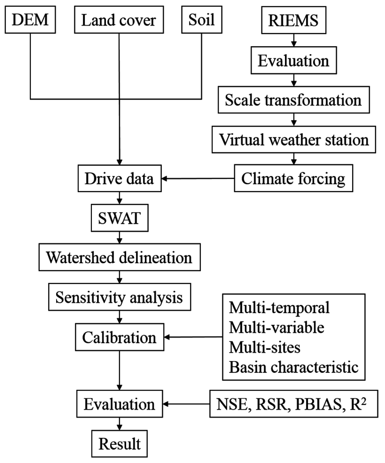
RIEMS evaluation and SWAT simulation were conducted in this study. First, we performed RIEMS evaluation, which is a precondition step of the coupled climate–hydrological model. Second, weather input parameters were prepared by scale transformation and climate parameter calculation and virtual weather stations, which served as climate forcing input parameters for SWAT, were used based on RIEMS; Next, coupling model simulation could be done accordingly. Further, a comprehensive hydrological calibration of SWAT had been selected. Finally, simulation results were evaluated according to certain criteria. Figure 3 shows a flowchart describing the model coupling method.

3.1. SWAT Hydrological Model

SWAT model is a physically based, semi-distributed hydrological model developed by United States Department of Agriculture. The model is used to simulate watershed movement in water, sediments, nutrients, etc. [37]. Two parts were included in the SWAT hydrological simulation. The first part consists of land areas that control water transported to channels together with other bodies of water, sediments, nutrients, and so on. The second part includes movements of water and sediment through stream networks to watershed outlets [38]. A watershed is divided into multiple subwatersheds that are further divided into hydrologic response units (HRUs). HRUs are basic elements for hydrological calculation, which integrate land areas with unique land cover, soil type, and slope combinations. Calculation of HRU hydrological balance is based on precipitation, evapotranspiration, surface runoff, groundwater flow, and so on. The hydrological cycle is simulated by SWAT based on water balance equation, which is as follows:
S W t , i = S W 0 , i + i = 1 t ( Q d a y , i Q s u r f , i E a , i W s e e p , i Q g w , i )
where SWt,i is final soil water content (mm H2O), SW0,i is initial soil water content on day i (mm H2O), t is time (days), Qday,i is precipitation amount of precipitation on day i (mm H2O), Qsurf,i is surface runoff amount on day i (mm H2O), Ea,i is amount of evapotranspiration on day i (mm H2O), Wseep,i is amount of water that enters vadose zone from soil profile on day i (mm H2O), and Qgw,i is return flow amount on day i (mm H2O).

3.2. RIEMS RCM

RIEMS RCM was designed and developed by START TEA-COM RRC and Department of Atmospheric Science of Nanjing University. RIEMS, which is a grid-based, terrain-following model, can be used to describe regional characteristics of East Asia [39]. RIEMS includes dynamical component of mesoscale model 5 [40], biosphere-atmosphere transfer scheme for land surface process representation, cumulus parameterisation [41,42,43], and modified radiation package of community climate model 3 [44].
HRB-observed datasets and remote sensing data were used to recalibrate RIEMS parameters, which include topography elevation, land cover type, saturated soil water potential, saturated soil hydraulic conductivity, field moisture capacity, wilting point moisture, soil porosity, and parameter b of soil hydraulic conductivity [45]. The high-resolution topographic dataset, vegetation classification data and land surface process parameters provided by United States Geological Survey (USGS) and Cold and Arid Regions Science Data Centre at Lanzhou, China. A high-resolution RCM was built for HRB with spatial and temporal resolutions of 3 km × 3 km and 6 h, respectively. This high-resolution RCM based on RIEMS was used to compensate for the deficiency of meteorological observation dataset and to drive the ecological–hydrological model in HRB.

3.3. Coupling Method

The purpose of the coupling method is to capture spatial heterogeneity of regional weather conditions in detail. One-way coupling is the climate model used as a forcing function to drive the hydrological model [46,47]. In this study, we proposed a one-way coupling method by building abundant and evenly distributed virtual weather stations based on RIEMS. SWAT was directly coupled with RIEMS by using virtual weather stations data that served as SWAT input parameters. Then, climate model evaluation and climate-forcing data processing were conducted to drive the SWAT model simulation of the runoff process.

3.4. Scale Transformation

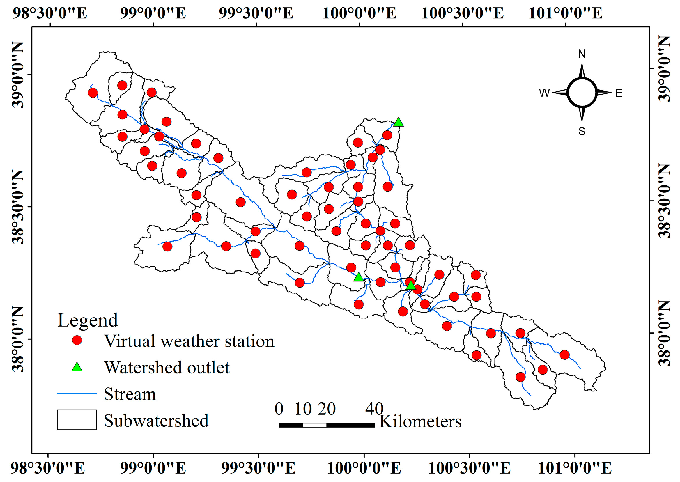
Scale transformation was conducted to match the climate-forcing data with the SWAT format. Scale transformation includes temporal and spatial scale transformations. In temporal scale transformation, the SWAT model needs daily climate data; we used a cumulative summation method to convert 6 h interval climate model data into 24 h interval. In terms of spatial scale transformation, the SWAT model generates many subwatersheds after watershed delineation, each subwatersheds reads the data of the station which is closest to its centre. Then, 3 km × 3 km grid climate model data were converted into 3 km × 3 km point datasets, and the virtual weather stations were built according to the location of subwatersheds and the number of subwatersheds.

3.5. Calibration and Validation

In this study, January 1995 to December 1998 were taken as warm-up periods. Periods from January 1998 to December 2004 and January 2005 to December 2010 were taken as calibration and validation periods, respectively. Calibration is the most important steps in model setup. According to natural basin characteristics, a data-deficient basin should be calibrated to the model with principles of multi-temporal, multi-variable, and multi-site calibration, which can improve the runoff simulation [5] Multi-temporal calibration for hydrological process was first conducted to average annual values, and then shifted to monthly average annual values. Multi-variable calibration for calibrated model parameters includes surface runoff, lateral flow, underground water, and evaporation simulation values. Calibration simulation values that are only based on observed data are avoided, and the hydrological process can be described properly. Multi-site calibration using the hydrological data of multiple sites on spacing started from the upstream to the downstream, and it did not change the calibrated parameters in the upstream catchment site. Calibration based on natural basin characteristics should be further developed to help calibrate the model better.

3.6. Statistical Evaluation Criteria

Model performances were evaluated with four different measures, which include Nash–Sutcliffe efficiency (NSE), root-mean-square-error-observation standard deviation ratio (RSR), percent bias (PBIAS), and determination coefficient (R2) [48,49,50,51]. These criteria are widely used in hydrological model studies [52,53]. Calculation processes are as follows:
NSE = 1 i = 1 n ( Q i o b s Q i s i m ) 2 i = 1 n ( Q i o b s Q a v g o b s ) 2
RSR = RMSE STDEV o b s = i = 1 n ( Q i o b s Q i s i m ) 2 i = 1 n ( Q i o b s Q a v g o b s ) 2
PBIAS = i = 1 n ( Q i o b s Q i s i m ) i = 1 n Q i o b s × 100
R 2 = [ i = 1 n ( Q i o b s Q a v g o b s ) ( Q i s i m Q a v g s i m ) ] 2 i = 1 n ( Q i o b s Q a v g o b s ) 2 i = 1 n ( Q i s i m Q a v g o b s ) 2
where Q i s i m is simulated streamflow, and Q i o b s is observed streamflow at time step i; whereas Q a v g o b s and Q a v g s i m are average observed and simulated streamflow values, respectively, in time periods 1, 2, …, n.
For NSE, average observation data are used to measure the representation of simulation values. The NSE range is from −∞ to 1, and its optimal value is 1 [48]. For RSR, measured values are used to standardise RMSE and integrate the advantages of error statistics. RSR ranges from 0 to 1. PBIAS measures the average tendency of simulated values. Positive values show overestimation and negative values indicate underestimation; the optimal value is 0 [50]. R2 ranges from 0 to 1; it represents the proportion of total variance in observation values. Simulation results with higher R2 show better model performance [36]. Monthly runoff evaluation standards are summarised in Table 3 [48].

4. Results

4.1. RIEMS Evaluation

RIEMS evaluation is a precondition of coupled climate–hydrological coupling. Accurate weather data can fairly represent regional climate conditions. It can also help to improve runoff simulation effects to conduct hydrology analysis and scenario predictions. High-resolution RCM based on RIEMS has been applied in HRB and focused on the applicability of simulated precipitation. In the upper reaches of HRB, various observation datasets were used for RIEMS evaluation. Precipitation was evaluated against meteorological observation station dataset. Simulated precipitation was overestimated in the upper reaches of HRB, with a bias of about 8.21%. The precipitation bias range is −1.6% to 34.3%, which is mostly consistent with IPCC report [54]. Correlation coefficients between simulation and observation data were 0.81, reaching the 0.01 significance level. Compared with the global monthly gridded climate data for precipitation averaged, the spatial correlation coefficient was 0.88, and significant at the 99% confidence level [55]. High-resolution RCM based on RIEMS can also simulate the spatial distribution characteristics of regional precipitation.
The evaluation of temperature, wind speed, and specific humidity is also important for hydrological simulation. A terrain representative index, the terrain representation of station using thiessen polygon method and the ones in the elevation zones, were analyzed to quantify the level of terrain representation of the climate stations [56]. After terrain representative analysis of climate stations, we selected the most representative Zhangye station to compare with monthly simulation and monthly observation data from 1995 to 2010. A scatter diagram of temperature, specific humidity, and wind speed is shown in Figure 4. Three climate parameters were all underestimated for observation, but the fitted line is close to 1. Wind-speed dispersive degree is the highest, and temperature aggregation degree is the best. The fitted line of the wind speed slope is separated from the diagonal line, which suggests that the simulated value is less than the observed value.
Slopes (a), correlation coefficients (r), RMSE, RSR, and PBIAS are shown in Table 4. Temperature, specific humidity, and wind speed of correlation coefficient reaches 0.93 and 0.01 significance levels. Specific humidity RMSE is the minimum, followed by temperature, and wind speed is the worst. RSR and PBIAS values of temperature are minimum and wind speed RSR is maximum, but it does not exceed 0.5. The specific humidity simulation value is greater than the observed value, and its overall deviation is the largest. Based on the evaluation results, a high-resolution RCM based on RIEMS has superior capability to capture basin climate variability.

4.2. Watershed Delineation

SWAT and RIEMS were coupled by building abundant and relatively evenly distributed virtual weather stations. Virtual weather stations, which served as input parameters to drive the SWAT simulation runoff process, were used to optimise the SWAT model weather input parameters. The efficiency of using high-resolution RCM data was restricted by the number of subwatersheds. Catchment area thresholds were used to define the watershed. The catchment area of watershed delineation was as small as theoretically possible. Based on the Alpine Mountain River, the best catchment threshold in the upper reaches of HRB [57], 80 km2 was selected as catchment area thresholds. Watershed outlet was set at Yingluoxia Hydrological Station, which controlled mountainous watershed runoffs. Two other outlets were set at Qilian and Zhamashike hydrological stations, which controlled the runoffs in the watershed of eastern and western tributaries, respectively. Finally, the watershed was divided into 3 hydrological regions and 61 subwatersheds. The 61 evenly distributed virtual weather stations were built, as shown in Figure 5.

4.3. Sensitivity Analysis and Calibration

Sensitivity analysis is an important method to understand how model parameters affect output variables [5]. It is used to calibrate the model with target. In this study, sensitivity analysis was conducted by using model parameters extracted from calibrated instructions of SWAT model user’s manual [58].
In the SWAT model, 26 parameters were sensitive to the hydrological process. Every value was difficult to confirm. Thus, we adjusted the parameters with high sensitivity to achieve optimal simulation results [59]. The 10 most sensitive parameters (Table 5) extracted from the 26 parameters were analysed. Among the 10 parameters, Cn2 is the most sensitive, followed by Tlaps, which determines surface runoff. Esco and Sol_Z determine soil water. Compared with the results of previous studies, lateral flow and baseflow have important contributions on the runoff in the upper reaches of HRB [16,18], while Alpah_Bf, Sol_K, Sol_Awc, and Ch_K2 are important in hydrological simulation. Then, Canmax and Bali determine interception. The watershed is located in a high and cold mountainous region. Snowfall and perennial snow also account for important contributions to the watershed. The parameters of the snow-melting process are also important.

4.4. Simulation Results and Applicability Assessment

The calibration procedure was based on natural basin characteristics and followed the principles of multi-temporal, multi-variable, and multi-site calibration method. Figure 6 shows the fitting results of monthly simulation and observation runoffs at Yingluoxia, Qilian, and Zhamashike hydrological stations. Results show that simulation values are close to observation values, and that the model performed well during a drought period, but exhibited a certain bias during wet season runoff simulation. In some years, the peak value had been overestimated.
Table 6 shows the evaluation results of runoff simulations of four assessment parameters. SWAT monthly simulation results show that NSEs are higher than 0.65. Yingluoxia has the best result, which reaches 0.82, during the validation period. RSRs are less than 0.65. PBIAS is controlled in the range of ±10%, except for the Zhamashike validation period that exceeded ±15%. R2 values are higher than 0.70, with Yingluoxia having the best result during the validation period at 0.83. The simulation results effectively indicated that the coupled climate–hydrological model is suitable for simulating runoff in the upper reaches of the HRB and that the model can provide an improved understanding of regional hydrological processes.

5. Discussion

Most of the previous studies used large- or meso-scale climate models that served as input parameters for the hydrological model [11,12,13]. Distributed hydrological simulations require a mass of high spatial and temporal resolutions of weather input parameters, which causes difficulty in meeting the requirements of hydrological simulation because of their coarse spatial resolution. The upper reaches of HRB only have six unevenly distributed meteorological observation stations. In this study, we used a high-resolution RCM based on RIEMS, with spatial and temporal resolutions reaching 3 km × 3 km and 6 h, respectively. RIEMS and SWAT were coupled by building abundant and evenly distributed virtual weather stations. Hydrological simulation achieved a good result, thereby indicating that RIEMS–SWAT coupling has optimised weather input data for hydrological simulation. In addition, the coupling model can provide scientific support for prediction and management of basin water resources.
According to previous studies, hydrological simulation application in the upper reaches of HRB has achieved satisfactory results [3,5,19,20,
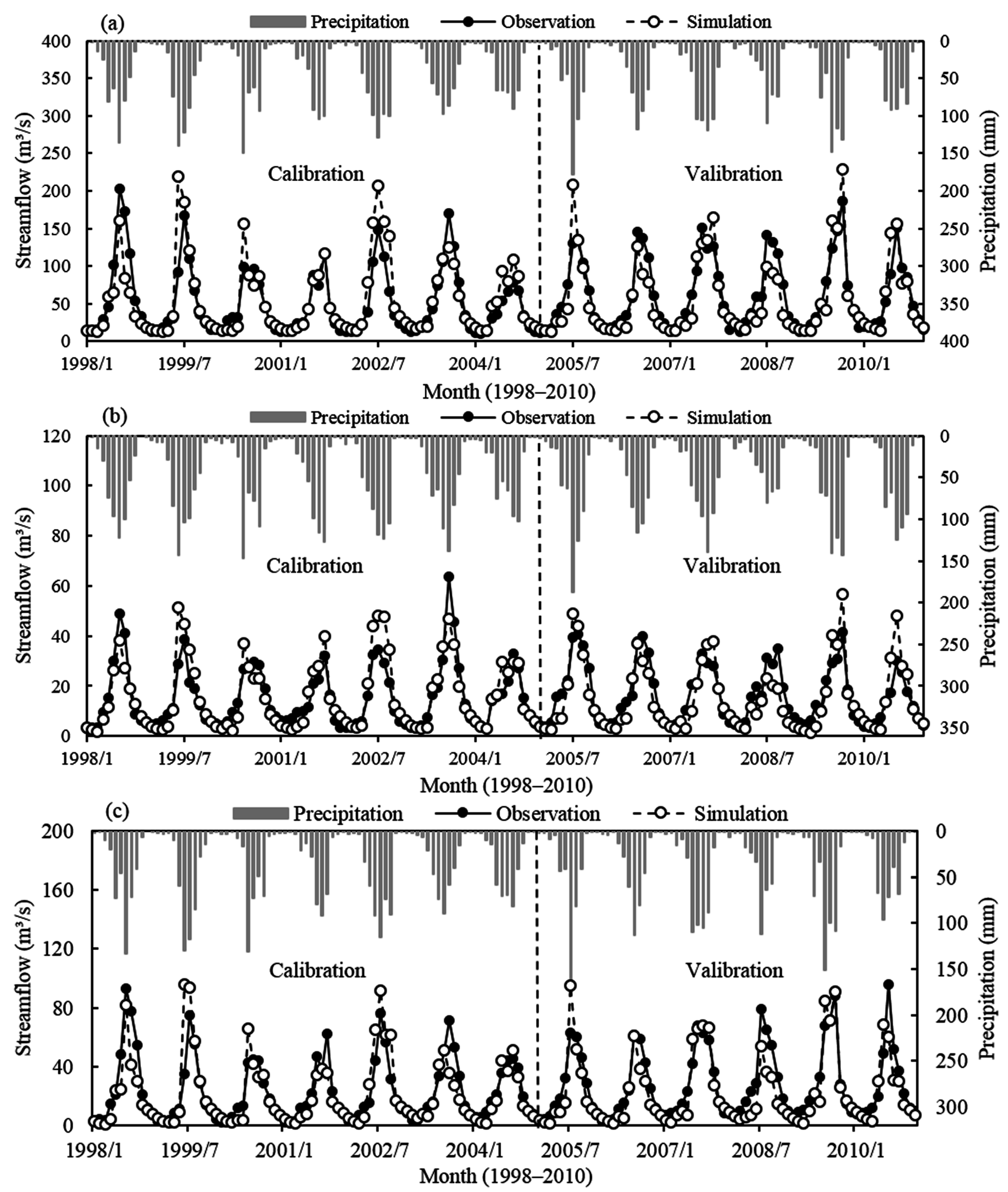
21]. However, this study has certain limitations compared with previous studies. The coupling model exhibits good performance during the drought season, but runoff simulation had a certain bias during the wet season, especially in some years when the peak value had been overestimated (
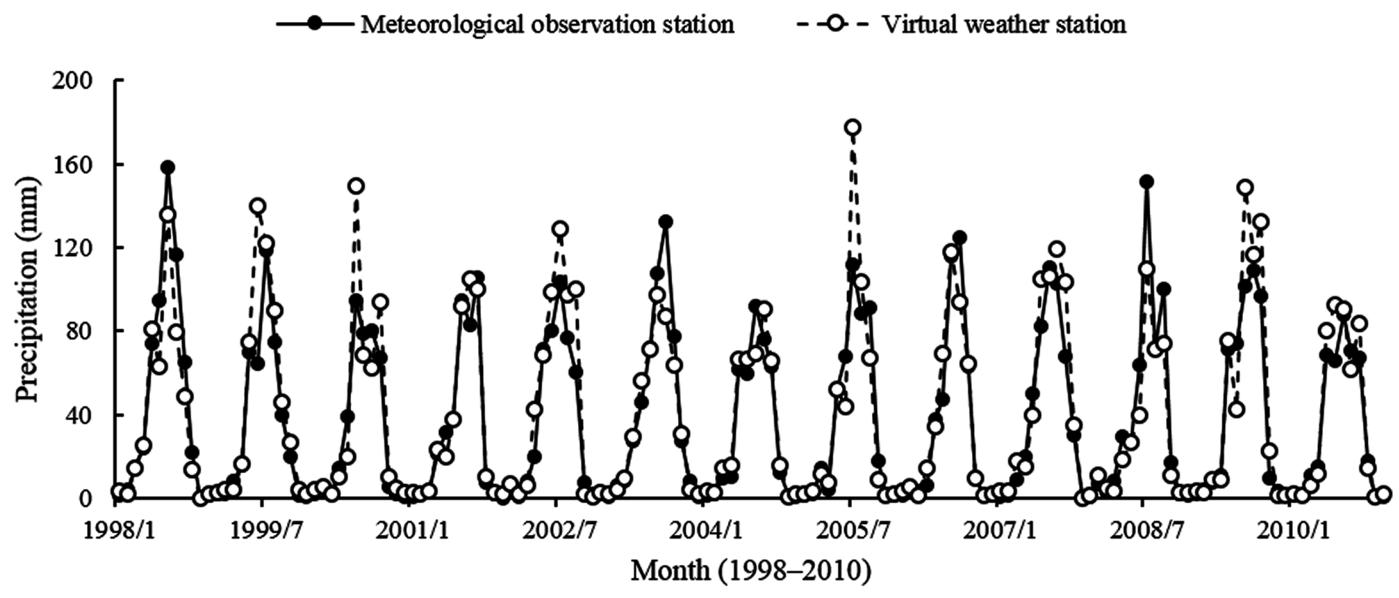
Figure 6). We used virtual weather stations and meteorological observation stations that serve as input parameters for SWAT, and the SWAT model exports two results of basin monthly average precipitation (Figure 7). Precipitation of the meteorological observation station is close to that of the virtual weather station. However, during wet seasons in 1999, 2002, 2005, and 2009, virtual weather station precipitation was apparently higher than those of meteorological observation stations. Compared with previous findings on watershed characteristics of precipitation, precipitation was overestimated by RIEMS in these periods [1,36], which was mostly consistent with the runoff simulation performance and RIEMS evaluation results. It is worth noting that specific humidity cannot be directly used by the SWAT model, we used an empirical formula to calculate relative humidity from specific humidity. To some extent, it has formed the error transfer and influenced the final simulation results.
Further research on enhancing simulation capability of coupled climate–hydrological model is needed. Weather input parameters are important in hydrological simulation. Further, improving the spatial description capability of high-resolution RCM in the upper reaches of HRB is necessary. In addition, the spatial discretisation scheme of the SWAT model based on weather stations failed to fully utilise high-resolution RCM data. Thus, it should be modified to adopt a grid-based discretisation scheme for hydrological simulation. Weather input parameters should also properly reflect the spatial heterogeneity of regional climate conditions. Ultimately, this study selected a one-way coupling method, where a climate model was used as a forcing function to drive the hydrological model, and there was no feedback from the land surface to the climate system. The climate model and hydrological model run independently, and the determination of land surface parameters of two models are different, so the calculation of evaporation and soil water is not same. Two models cannot share the land surface simulation results, where the hydrological model cannot use climate forcing to improve the calculation of evaporation and soil water in real-time; the climate model cannot use hydrological simulation results to modify the precision of land surface process simulation result in real-time [60]. Conversely, the two-way coupling method allows feedback loop simulation, which can avoid the problem of one-way coupling. Thus, selecting the two-way coupling method would assist future research on soil-plant-atmosphere-hydrology interaction and fundamentally enhance the simulation effects of the coupled climate–hydrological model.

6. Conclusions

In this study, we proposed a climate and hydrological coupling model to properly understand the basin hydrological process. An integration method, which coupled the RIEMS RCM and SWAT hydrological model based on input data optimisation, was also presented. This model coupling can provide an effective attempt to compensate for the deficiency of meteorological observation stations. Developing a stronger model can be applied to watershed for runoff simulation.
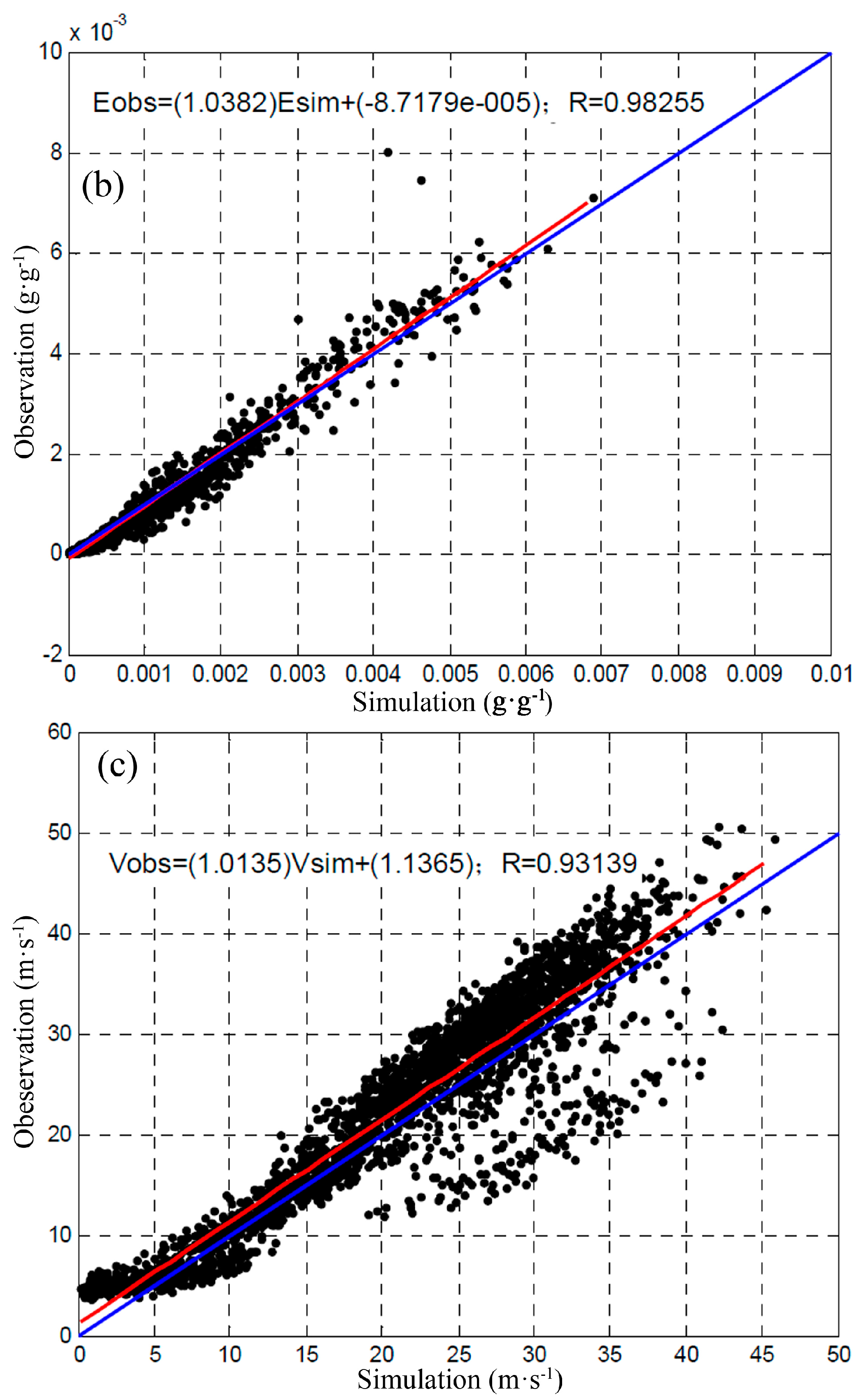
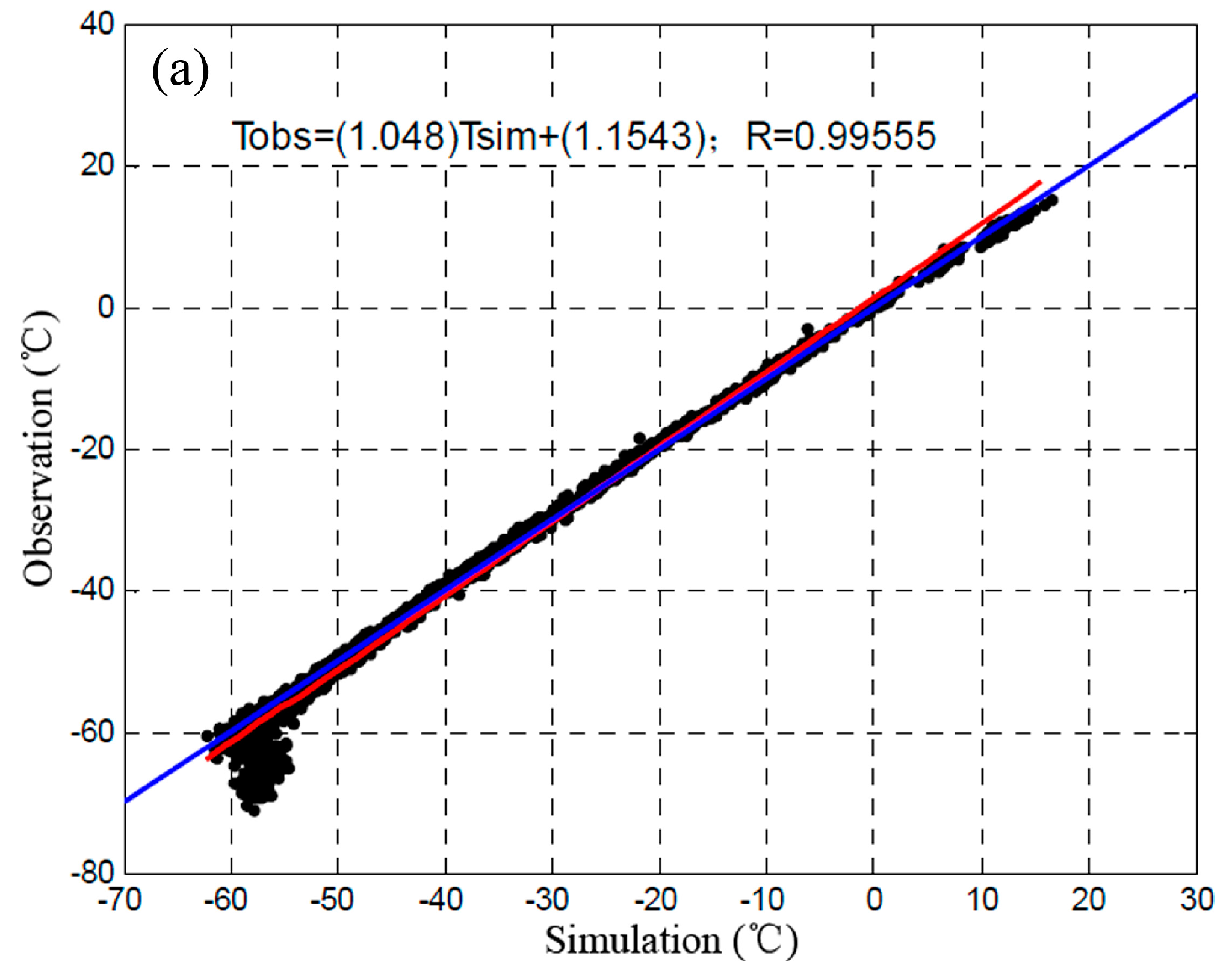
Before climate and hydrological model coupling, we verified the high-resolution RCM based on RIEMS with high resolution and precision. The correlation coefficients of precipitation, temperature, specific humidity, and wind speed are all above 0.8, with 0.01 significance levels. Spatial and temporal resolutions reached 3 km × 3 km and 6 h, respectively. RIEMS can represent watershed weather variability, but it has less satisfactory results with wet season precipitation of some years. In addition, we proposed a one-way coupling method by building abundant and evenly distributed virtual weather stations based on RIEMS. We also used the climate model that served as input parameters for the hydrological model. By using this method to capture spatial heterogeneity of weather variability accurately, deficiencies of scarce and unevenly distributed meteorological observations stations were compensated, and optimisation of SWAT weather input parameters was achieved. Considering the natural characteristics of watersheds, we followed the principles of multi-temporal calibration, multi-variable calibration, and multi-site calibration. We also simulated the monthly runoff process. According to statistical evaluation, NSEs were higher than 0.65, R2 values exceeded 0.70, PBIAS values were controlled in the range of ±20%, and RSRs were less than 0.65. These results prove that the coupling model has a fair applicability to simulate the runoff process in the upper reaches of HRB.
Future studies should focus on improving the numerical simulation accuracy of high-resolution RCM. We should also modify the spatial discretisation scheme of the hydrological model and choose the two-way coupling method. Developing the coupled climate–hydrological model research in the upper reaches of HRB will also contribute scientific support for the prediction and management of water resources, as well as assist in further research on the responses of water resources to global climate change and human activities.

Acknowledgments

This work was supported by the National Natural Science Foundation of China (41571031, 91425304, 91225302, 41601038, 41601036). The authors are grateful to the Cold and Arid Regions Science Data Centre at Lanzhou (http://westdc.westgis.ac.cn) for data support. The authors thank the academic editor and two anonymous reviewers for their constructive comments that have significantly improved this work, and thank Baorong Xu and Yi Zheng for data preprocessing and comments.

Author Contributions

Modeling and analysis was performed by Songbing Zou and Hongwei Ruan; the paper was written by Songbing Zou and Hongwei Ruan; critical data were provided by Dawen Yang and Zhe Xiong; and Zhixiang Lu and Zhenliang Yin made editing corrections and improvements to the manuscript.

Conflicts of Interest

The authors declare no conflict of interest.

References

  1. Deng, X.Z.; Shi, Q.L.; Zhang, Q.; Shi, C.C.; Yin, F. Impacts of land use and land cover changes on surface energy and water balance in the Heihe River Basin of China, 2000–2010. Phys. Chem. Earth A/B/C 2015, 79–82, 2–10. [Google Scholar] [CrossRef]
  2. Deng, X.Z.; Singh, R.B.; Liu, J.G.; Güneralp, B. Water use efficiency and integrated water resource management for river basin. Phys. Chem. Earth 2015, 89, 1–2. [Google Scholar] [CrossRef]
  3. Kang, E.S.; Cheng, G.D.; Lan, Y.C.; Jin, H.J. A model for simulating the response of runoff from the mountainous watershed of inland river basins in the arid area of northwest China to climatic changes. Sci. China Ser. D 1999, 42, 52–63. [Google Scholar] [CrossRef]
  4. Yu, M.Y.; Chen, X.; Li, L.H.; Bao, A.M.; Paix, M.J. Streamflow simulation by SWAT using different precipitation sources in large arid basins with scarce raingauges. Water Resour. Manag. 2011, 25, 2669–2681. [Google Scholar] [CrossRef]
  5. Lu, Z.X.; Zou, S.B.; Xiao, H.L.; Zheng, C.M.; Yin, Z.L.; Wang, W.H. Comprehensive hydrologic calibration of SWAT and water balance analysis in mountainous watersheds in northwest China. Phys. Chem. Earth A/B/C 2015, 79–82, 76–85. [Google Scholar] [CrossRef]
  6. Chen, J.F.; Zhang, W.C.; Gao, J.F.; Cao, K. Assimilating multi-site measurements for semi-distributed hydrological model updating. Quat. Int. 2012, 282, 122–129. [Google Scholar] [CrossRef]
  7. Shie, Y.L.; Raghavan, S.V.; Vu, M.T. Climate Change and Its Impacts on Streamflow: WRF and SCE-Optimized SWAT Models. Data Assim. Atmos. Ocean. Hydrol. Appl. 2013, 2, 411–428. [Google Scholar]
  8. Oyerinde, G.T.; Hountondji, F.C.; Wisser, D.; Diekkruger, B.; Lawin, A.E.; Odofin, A.J.; Afouda, A. Hydro-climatic changes in the Niger basin and consistency of local perceptions. Reg. Environ. Chang. 2015, 15, 1627–1637. [Google Scholar] [CrossRef]
  9. Huang, L.; Xu, X.L.; Zhai, J.; Sun, C.Y. Local background climate determining the dynamics of plateau lakes in China. Reg. Environ. Chang. 2016, 1–14. [Google Scholar] [CrossRef]
  10. Scoccimarro, E.; Gualdi, S.; Bellucci, A.; Zampieri, M.; Navarra, A. Heavy precipitation events over the Euro-Mediterranean region Heavy precipitation events over the Euro-Mediterranean region. Reg. Environ. Chang. 2016, 16, 595–602. [Google Scholar] [CrossRef]
  11. Lakhtakia, M.N.; Yarnal, B.; Johnson, D.L.; White, R.A.; Miller, D.A.; Yu, Z. A simulation of river-basin response to mesoscale meteorological forcing: The Subsequenhanna River Basin Experiment (SRBEX). JAWRA 1998, 43, 921–937. [Google Scholar] [CrossRef]
  12. Evans, J.P. Improving the characteristics of stream flow modeled by regional climate models. J. Hydrol. 2003, 284, 211–227. [Google Scholar] [CrossRef]
  13. Christensen, N.S.; Lettenmaier, D.P. A multimodel ensemble approach to assessment of climate change impacts on the hydrology and water resources of the Colorado River Basin Hydrol. Earth Syst. Sci. 2007, 11, 1417–1434. [Google Scholar] [CrossRef]
  14. Wang, N.L.; Zhang, S.B.; He, J.Q.; Pu, J.C.; Xu, X.B.; Jiang, X. Tracing the major source area of the mountainous runoff generation of the Heihe River in northwest China using stable isotope technique. Chin. Sci. Bull. 2009, 54, 2751–2757. [Google Scholar] [CrossRef]
  15. Pan, X.D.; Li, X. Validation of WRF model on simulating forcing data for Heihe River Basin. Sci. Cold Arid Reg. 2011, 3, 344–357. [Google Scholar]
  16. Zhao, L.J.; Yin, L.; Xiao, H.L.; Cheng, G.D.; Zhou, M.X.; Yang, Y.G.; Li, Z.C.; Zhou, J. Isotopic evidence for the moisture origin and composition of surface runoff in the headwater of the Heihe River basin. Chin. Sci. Bull. 2011, 56, 58–67. [Google Scholar] [CrossRef]
  17. Li, Z.L.; Xu, Z.X.; Li, Z.J. Performance of WASMOD and SWAT on hydrological simulation in Yingluoxia watershed in nourthwest of China. Hydrol. Process. 2011, 25, 2001–2008. [Google Scholar] [CrossRef]
  18. Li, Z.L.; Shao, Q.X.; Xu, Z.X.; Cai, X.T. Analysis of parameter uncertainty in semidistributed hydrological models using bootstrap method: A case study of SWAT model applied to Yingluoxia watershed in northwest China. J. Hydrol. 2010, 385, 76–83. [Google Scholar] [CrossRef]
  19. Li, Z.L.; Xu, Z.X.; Shao, Q.X.; Yang, J. Parameter estimation and uncertainty analysis of SWAT model in upper reaches of the Heihe river basin. Hydrol. Process. 2009, 23, 2744–2753. [Google Scholar] [CrossRef]
  20. Giorgi, F. Simulations of regional climate using a limited area model nested in a general circulation model. J. Clim. 1990, 3, 941–963. [Google Scholar] [CrossRef]
  21. Deng, X.Z.; Singh, R.B.; Liu, J.G.; Güneralp, B. Physical and economic processes of water scarcity and water allocation for integrated river basin management. Phys. Chem. Earth A/B/C 2015, 79. [Google Scholar] [CrossRef]
  22. Huang, J.; Dool, H.M.; Georgakakos, K.P. Analysis of model-calculated soil moisture over the United States (1931–1993) and application to long-range temperature forecasts. J. Clim. 1996, 9, 1350–1362. [Google Scholar] [CrossRef]
  23. Arnold, J.G.; Srinivasan, R.; Muttiah, R.S.; Williams, J.R. Large area hydrologic modeling and assessment: Part I. Model development. J. Am. Water Resour. Assoc. 1998, 34, 73–89. [Google Scholar] [CrossRef]
  24. Liu, Y.Q.; Xu, Z.M.; Nan, Z.T. Study on ecological compensation in upper stream of Heihe River Basin based on SWAT model and minimum-data approach. Trans. Chin. Soc. Agric. Eng. 2012, 28, 124–130. [Google Scholar]
  25. Shi, P.; Ma, X.X.; Hou, Y.B.; Li, Q.F.; Zhang, Z.C.; Qu, S.M.; Chen, C.; Cai, T.; Fang, X.Q. Effects of land-use and climate change on hydrological processes in the upstream of Huai River, China. Water Resour. Manag. 2013, 27, 1263–1278. [Google Scholar] [CrossRef]
  26. Glavan, M.; Ceglar, A.; Pintar, M. Assessing the impacts of climate change on water quantity and quality modelling in small Slovenian Mediterranean catchment–lesson for policy and decision makers. Hydrol. Process. 2015, 29, 3124–3144. [Google Scholar] [CrossRef]
  27. Tokar, A.S.; Markus, M. Precipitation-runoff modeling using artificial neural networks and conceptual models. ASCE J. Hydrol. Eng. 2000, 5, 156–161. [Google Scholar] [CrossRef]
  28. Rezaeianzadeh, M.; Stein, A.; Tabari, H.; Abghari, H.; Jalalkamali, N.; Hosseinipour, E.Z.; Singh, V.P. Assessment of a conceptual hydrological model and artificial neural networks for daily outflows forecasting. Int. J. Environ. Sci. Technol. 2013, 10, 1181–1192. [Google Scholar] [CrossRef]
  29. Makwana, J.J.; Tiwari, M.K. Intermittent streamflow forecasting and extreme event modelling using wavelet based artificial neural networks. Water Resour. Manag. 2014, 28, 4857–4873. [Google Scholar] [CrossRef]
  30. Navideh, N.; Latif, K. Coupling SWAT and ANN models for enhanced daily streamflow prediction. J. Hydrol. 2016, 533, 141–151. [Google Scholar]
  31. Xiong, Z.; Wang, S.Y.; Zeng, Z.M.; Fu, C.B. Analysis of simulated heavy rain over the Yangtze River Valley During 11–30 June 1998 using RIEMS. Adv. Atmos. Sci. 2003, 20, 815–824. [Google Scholar]
  32. Zhang, J.Y.; Dong, W.J.; Fu, C.B.; Wu, L.Y.; Xiong, Z.; Ma, J.; Zhang, K.J. Streamflow simulation for the yellow river basin using RIEMS and LRM. Adv. Atmos. Sci. 2003, 20, 415–424. [Google Scholar] [CrossRef]
  33. Yong, B.; Ren, L.L.; Chen, X.; Zhang, Y.; Zhang, W.C.; Fu, C.B.; Niu, G.Y. Development of a large-scale hydrological model TOPX and its coupling with regional integrated environment modeling system RIEMS. Chin. J. Geophys. 2009, 52, 1954–1965. [Google Scholar] [CrossRef]
  34. Zang, C.F.; Liu, J.G. Trend analysis for the flows of green and blue water in the Heihe River basin, northwestern China. J. Hydrol. 2013, 502, 27–36. [Google Scholar] [CrossRef]
  35. Wu, F.; Zhan, J.Y.; Wang, Z.; Zhang, Q. Streamflow variation due to glacier melting and climate change in upstream Heihe River Basin, Northwest China. Phys. Chem. Earth 2015, 79, 11–19. [Google Scholar] [CrossRef]
  36. Yin, Z.L.; Xiao, H.L.; Zou, S.B.; Zhu, R.; Lan, Y.C.; Shen, Y.P. Simulation of hydrological process of mountainous watersheds in inland river basin: Taking the Heihe Mainstream River as an example. J. Arid Land 2014, 6, 16–26. [Google Scholar] [CrossRef]
  37. Arnold, J.G.; Moriasi, D.N.; Gassman, P.W.; Abbaspour, K.C.; White, M.J.; Srinivasan, R.; Santhi, C.; Harmel, R.D.; Van Griensven, A.; Van Liew, M.W.; et al. SWAT: Model use, calibration, and validation. ASABE 2012, 55, 1491–1508. [Google Scholar] [CrossRef]
  38. Neitsch, S.; Arnold, J.; Kiniry, J.; Williams, J. Soil and Water Assessment Tool Theoretical Documentation, version 2009; Blackland Research Center, Texas Agricultural Experiment Station: Temple, TX, USA, 2011. [Google Scholar]
  39. Fu, C.B.; Yuan, H.L. A virtual numerical experiment to understand the impacts of recovering natural vegetation on the summer climate and environmental conditions in East Asia. Chin. Sci. Bull. 2001, 46, 1199–1203. [Google Scholar] [CrossRef]
  40. Grell, G.A.; Dudhia, J.; Stauffer, D. A Description of the Fifth-Generation Penn State/NCAR Mesoscale Model (MM5). NCAR Technical Note NCAR/TN-398+STR. Available online: http://opensky.ucar.edu/islandora/object/technotes:170 (accessed on 13 October 2016).
  41. Fritsch, J.M.; Chappell, C.F. Numberical prediction of convectively driven mesoscale pressure system. Part I: Convective parameterization. J. Atmos. Sci. 1980, 37, 1722–1733. [Google Scholar] [CrossRef]
  42. Dickinson, R.E.; Henderson, S.A.; Kennedy, P.J. Biosphere-Atmosphere Transfer Scheme (BATS) Version as Coupled to the NCAR Community Climate Model. NCAR Technical Report NCAR/TN-387+STR. Available online: https://opensky.ucar.edu/islandora/object/technotes%3A154 (accessed on 13 October 2016).
  43. Grell, G.A. Prognostic evaluation of assumptions used by cumulus parameterizations. Mon. Weather Rev. 1993, 121, 764–787. [Google Scholar] [CrossRef]
  44. Kiehl, J.T.; Hack, J.J.; Bonan, G.B.; Boville, B.A.; Briegleb, B.P.; Williamson, D.L.; Rasch, P.J. Description of the NCAR Community Climate Model (CCM3). NCAR Technical Note NCAR/TN-420+STR. Available online: https://opensky.ucar.edu/islandora/object/technotes%3A187 (accessed on 13 October 2016).
  45. Xiong, Z. Simulated forcing dataset of 3 km/6 hour in 1980–2010 in Heihe River Basin. Heihe Plan Sci. Data Center 2014. [Google Scholar] [CrossRef]
  46. Molders, N.; Raabe, A. Testing the effect of a two-way-coupling of meteorological and a hydrologic model on the predicted local weather. Atmos. Res. 1997, 45, 81–107. [Google Scholar] [CrossRef]
  47. Goodall, J.L.; Saint, K.D.; Ercan, M.B.; Briely, L.J.; Murpy, S.; You, H.H.; Deluca, C.; Rood, R.B. Coupling climate and hydrological models: Interoperability through Web Services. Environ. Model. Softw. 2013, 46, 250–259. [Google Scholar] [CrossRef]
  48. Nash, J.E.; Sutcliffe, J.V. River flow forecasting through conceptual models: Part 1. A discussion of principles. J. Hydrol. 1970, 10, 282–290. [Google Scholar] [CrossRef]
  49. Legates, D.R.; McCabe, J. Evaluating the use of “Goodness-of-Fit” measures in hydrologic and hydroclimatic model validation. Water Resour. Res. 1999, 35, 233–241. [Google Scholar] [CrossRef]
  50. Gupta, H.V.; Sorooshian, S.; Yapo, P.O. Status of automatic calibration for hydrologic models: Comparison with multilevel expert calibration. J. Hydrol. Eng. 1999, 4, 135–143. [Google Scholar] [CrossRef]
  51. Singh, J.; Knapp, H.V.; Arnold, J.G.; Demissie, M. Hydrologic modeling of the Iroquois River watershed using HSPF and SWAT. J. Am. Water Resour. Assoc. 2005, 41, 343–360. [Google Scholar] [CrossRef]
  52. Krause, P.; Boyle, D.P.; Bäse, F. Comparison of different efficiency criteria for hydrological model assessment. Adv. Geosci. 2005, 5, 89–97. [Google Scholar] [CrossRef]
  53. Moriasi, D.N.; Arnold, J.G.; Van Liew, M.W.; Bingner, R.L.; Harmel, R.D.; Veith, T.L. Model evaluation guidelines for systematic quantification of accuracy in watershed simulations. Trans. ASABE 2007, 50, 885–900. [Google Scholar] [CrossRef]
  54. Houghton, J.T. In The solar cycle and terrestrial climate, solar and space weather. IPCC Rep. 2001, 463, 255–259. [Google Scholar]
  55. Xiong, Z.; Yan, X.D. Building a high-resolution regional climate model for the Heihe River Basin and simulating precipitation over this region. Chin. Sci. Bull. 2013, 58, 4670–4678. [Google Scholar] [CrossRef]
  56. Xu, B.R.; Lu, Z.X.; Liu, S.Y.; Li, J.; Xie, J.L.; Long, A.H.; Yin, Z.L.; Zou, S.B. Glacier changes and their impacts on the discharge in the past half-century in Tekes watershed, Central Asia. Phys. Chem. Earth A/B/C 2015, 89, 96–103. [Google Scholar] [CrossRef]
  57. Lu, Z.X.; Zou, S.B.; Xiao, H.L.; Yin, Z.L.; Ruan, H.W.; Gao, H.S. How to determine drainage area threshold in alpine regions of upper reaches of Heihe River. J. Glaciol. Geocryol. 2015, 37, 493–499. [Google Scholar]
  58. Neitsch, S.; Arnold, J.; Kiniry, J.; King, K.; Williams, J. Soil and Water Assessment Tool (SWAT) Theoretical Documentation; BRC Report 02-05; Blackland Research Center, Texas Agricultural Experiment Station: Temple, TX, USA, 2005. [Google Scholar]
  59. Xu, B.R.; Zou, S.B.; Liu, Y.; Lu, Z.X.; Xiao, H.L. Terrain representation for the precipitation stations in Heihe River Basin based on GIS. J. Lanzhou Univ. (Nat. Sci.) 2015, 51, 166–172. [Google Scholar]
  60. Yang, C.G.; Lin, C.H.; Hao, Z.C.; Yu, Z.B.; Liu, S.F. Review of Coupling Atmospheric and Hydrological Models. Adv. Earth Sci. 2007, 22, 800–817. [Google Scholar]
Figure 1. Upper reaches of the Heihe River Basin.
Water 08 00455 g001
Figure 2. Distribution of soil types (a) and land cover types (b).
Water 08 00455 g002
Figure 3. Diagram of the SWAT and RIEMS model coupling method.
Water 08 00455 g003
Figure 4. Temperature scatter diagram (a); specific humidity (b); and wind speed (c) (The red line is fitted line, and the blue line is 1:1 diagonal line).
Water 08 00455 g004aWater 08 00455 g004b
Figure 5. Watershed delineation and distribution of virtual weather stations.
Water 08 00455 g005
Figure 6. Monthly observation and simulated runoff (a) Yingluoxia Station; (b) Qilian Station; (c) Zhamashike Station.
Water 08 00455 g006
Figure 7. Basin monthly precipitation from meteorological observation station and virtual weather station.
Water 08 00455 g007
Table 1. Code List of Soil Types.
CodeSoilDescriptionCodeSoilDescription
23111121GRCSGrey cinnamon soils23117104MEMSMeadow marsh soils
23111123LGCSLeaching grey cinnamon soils23117111LMPSLow moor peat soils
23112101CHERChernozem23120102ALMSAlpine meadow soils
23112112CHESChestnut soils23120104BAMSBrown alpine meadow soils
23112113LICSLight chestnut soils23120112DAFSDark felty soils
23113113MESIMeadow sierozem23120113TDFSThin dark felty soils
23115181CHISChisley soils23120114BDFSBrown dark felty soils
23115184CALICalcium lithosol23120122FRCSFrigid calcic soils
23116102LIMSLimy meadow soils23120132COCSCold calcic soils
23117101BOGSBog soils23120133DCCSDark cold calcic soils
23117102SAMSSapropel mire soils23120171FRFSFrigid frozen soils
23117103PEMSPeat mire soils23127101SNOWGlacier snow
Table 2. Code list of land cover types.
CodeLand CoverDescriptionCodeLand CoverDescription
14PICRPicea crassifolia415aSTPSStipa purpurea steppe
197HIRSHippophae rhamnoides scrubland497LWAMLittle wormwood alpine meadow
239SAGSSalix gilashanica scrubland498KHAMKobresia humilis alpine meadow
241SAOSSalix oritrepha scrubland503bKFKMKobresia folifolia alpine meadow
241aSOBCSalix oritrepha, bush cinquefoil scrubland504aTWSSTibet wormwood, sedge swamp alpine meadow
246BUCSBush cinquefoil scrubland506ENRNElymus nutans, roegneria nutans
312SYRDSympegma regelii desert556SMSSSaussurea medusa maxim, saussurea sparse vegetation
369STKSStipa krylovii steppe557SRHSSaussurea, rhodiola rosea, herba cremanthodium sparse vegetation
374LONSLooseflower needlegrass steppe561HSPRHighland barley, spring wheat, potato, round radish, pea, rape
375SBSBStipa breviflora, stipa bungeana steppeGsSNOWGlacier snow
Table 3. Monthly runoff evaluation standard.
StandardNSERSRPBIAS (%)
Very good0.75 < NSE ≤ 1.000.00 < RSR ≤ 0.50PBIAS < ±10
Good0.65 < NSE ≤ 0.750.50 < RSR ≤ 0.60±10 ≤ PBIAS < ±15
Satisfactory0.50 < NSE ≤ 0.650.60 < RSR ≤ 0.70±15 ≤ PBIAS < ±25
UnsatisfactoryNSE ≤ 0.50RSR > 0.7PBIAS ≥ ±25
Table 4. Simulated evaluation of temperature, specific humidity and wind speed.
ElementsarRMSERSRPBIAS
Temperature1.041.002.260.101.82
Specific humidity0.880.970.000.36−27.35
Wind speed0.930.934.080.426.77
Table 5. Most sensitive parameters.
ParameterDescriptionHydrologic ProcessRangeValueSensitive
Cn2Moisture condition curve numberSurface runoff−0.2–0.2−10–−61
TlapsTemperature lapse rate (°C/km)Snow fall and melt, evapotranspiration−15–15−5.52
Alpha_BfBaseflow recession constant Baseflow0–10.072–0.063
EscoSoil evaporation compensation factorSoil water and soil evaporation0–10.75–0.904
Sol_ZDepth from soil surface to bottom of layer (mm)Soil water0–3500100–17005
Ch_K2Effective hydraulic conductivity in main channel alluvium (mm/h)Concentration of channel−0.01–50013–356
Sol_AwcAvailable soil water capacity (mm/mm)Soil water0.01–0.40.02–0.047
Sol_KSaturated hydraulic conductivity of first layer (mm/h)Infiltration and soil water0–3000.15–0.28
BaliPotential maximum leaf area index for the plantInterception0–100.05–0.099
CanmxMaximum canopy storage (mm)Interception0–100.06–0.0910
Table 6. Evaluation of runoff simulation.
StationCalibration (January 1998–December 2004)Validation (January 2005–December 2010)
NSERSRPBIAS (%)R2NSERSRPBIAS (%)R2
Yingluoxia0.660.57−7.240.750.820.469.130.83
Qilian0.750.49−4.320.800.690.626.740.76
Zhamashike0.690.556.910.730.780.4418.340.81

