Terrestrial Sediment Yield Projection under the Bias-Corrected Nonstationary Scenarios with Hydrologic Extremes

Abstract

For reliable prediction of sediment yield in a watershed, fine-scale projections for hydro-climate components were first obtained using the statistical bias correction and downscaling scheme based on the combination of an Artificial Neural Network (ANN), Nonstationary Quantile Mapping (NSQM) and Stochastic Typhoon Synthesis (STS) sub-modules. Successively, the hydrologic runoff and sediment yield from the land surfaces were predicted through the long-term continuous watershed model, Soil and Water Assessment Tool (SWAT), using the bias-corrected and downscaled Regional Climate Model (RCM) output under the Intergovernmental Panel on Climate Change’s (IPCC’s) A1B climate change scenario. The incremental improvement of the combined downscaling process was evaluated successfully during the baseline period, which provides projected confidence for the simulated future scenario. The realistic simulation of sediment yield is closely related to the rainfall event with high intensity and frequency. During the long-term future period, the Coefficient of River Regime (CORR) reaches 353.9 (27.2% increase with respect to baseline). The projection for annual precipitation by 2040 and 2100 is a 25.7% and a 57.2% increase with respect to the baseline period, respectively. In particular, the increasing CORR rate (33.4% and 72.5%) during the flood season is much higher than that for the annual total amount. However, the sediment yield is expected to increase by 27.4% and 121.2% during the same periods, which exhibits steeper trends than the hydrologic runoff. The June, July, August (JJA) season occupies 83.0% annual total sediment yield during the baseline period, which is similar during the projection period. The relative change of sediment yield is 1.9-times higher than that of dam inflows.

1. Introduction

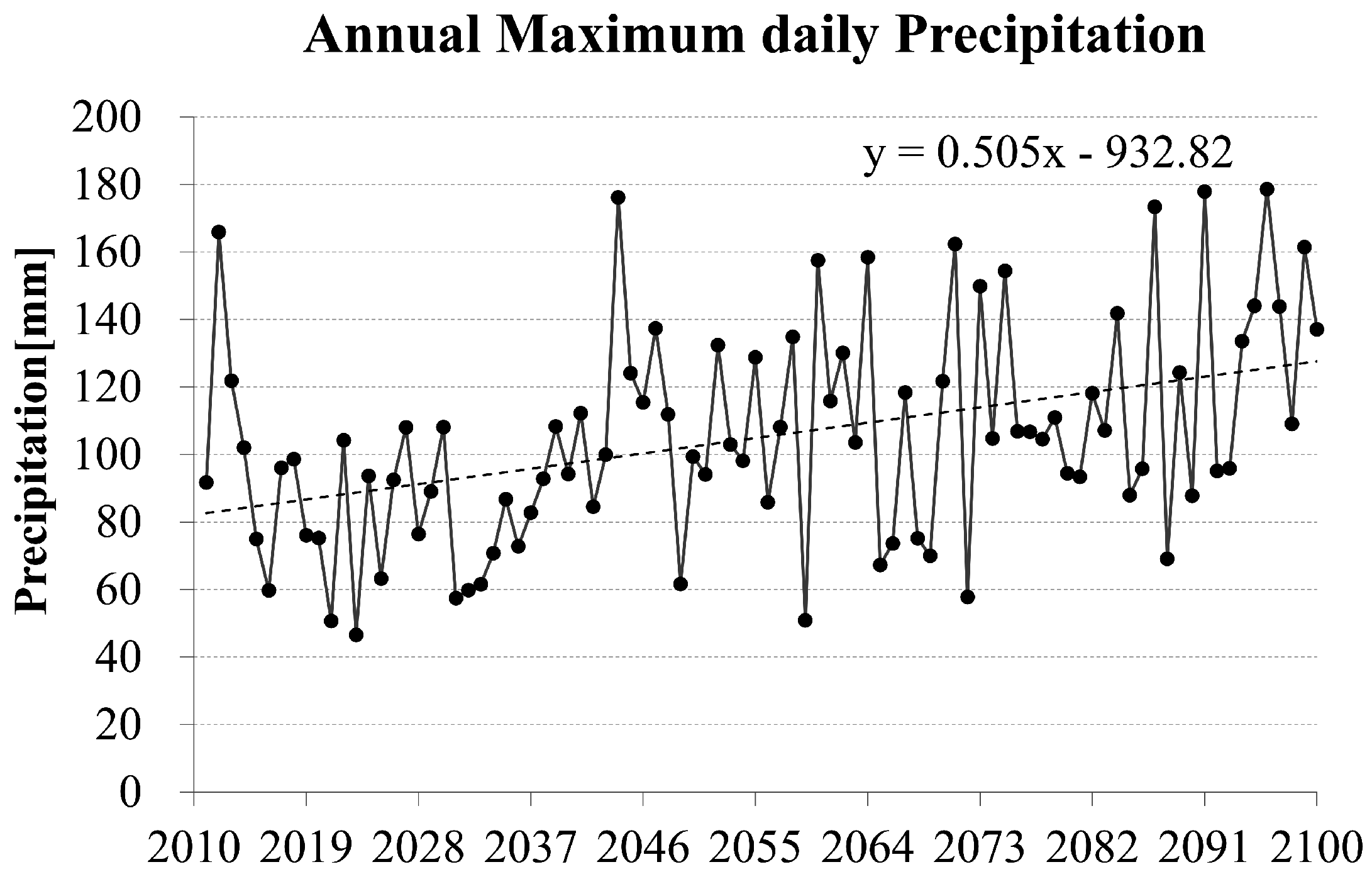
The major consequences of climate change in the Korean peninsula will be upward trends in mean atmospheric temperature and precipitation. The increase in the regional precipitation has been observed in the form of not only total precipitation, but also heavy precipitation events. Kang [1] reported that between 1973 and 2007, the average daily maximum precipitation increased 105.8 mm (38.5%), and the average occurrence of the storm events over 80 mm/day increased by 1.02 events (61.4%). Pruski and Nearing [2] found that a change in precipitation amount and intensity had a much greater effect on soil erosion and runoff generation than a change in storm frequency. The eroded sediments and sediment-bound chemicals from non-point sources, in particular, can enter the surface water system, resulting in long-term eutrophication and toxification [3].

However, the climate change impacts on erosion, sediment transport and deposition have been dealt with as research topics only recently. The primary limitation of soil erosion prediction under the climate change scenario is the spatial-temporal scale of available outputs Michael [3] and the Global Climate Model’s (GCM’s) limited capability of reproducing local extreme storm events and tropical cyclones, e.g., typhoon events.

Under the similar precipitation scenario, the impacts on sediment runoff show a different regime. In the New York City water supply watershed, the sediment yield is more significant during the winter season due to a shift in the timing of snowmelt (Mukundan et al., 2013). In most regions, a variation (increase/decrease) in future precipitation leads to the resultant same variation in soil erosion [4,5]. In spite of the increase of future summer precipitation, sediment yield during the summer season was predicted to decrease owing to an increase in soil moisture deficit and evapotranspiration, meaning an increase in precipitation loss [6]. In the case of central Oklahoma, U.S., the rate of increase in sediment runoff is revealed to depend more on the variability of precipitation. Even though the total annual precipitation increases in the future, the sediment runoff is expected to increase owing to the increased variability of precipitation, and the rate of increase in sediment was amplified compared with that in precipitation [7]. Asselman et al. [8] found that the sediment in the entire basin will increase in the future, but upstream and downstream reaches show different regimes, not only in the rate, but also in the increase or decrease due to the effectiveness of sediment delivery along the river courses.

Coupling hydro-climatic components with the physical process for sediment runoff is a key module for obtaining reliable projection. A few examples of coupling processes are the mechanistic understanding of the spatial and temporal evolution of the hydrodynamical sediment transport process and volumetric changes in suspended sediment and bedload [9]; dynamic interactions and feedbacks between the terrestrial biosphere and the water cycle [10]; experimental findings for the relationship between nutrient export and rainfall or runoff time distribution [11]. Typhoon rainfall is one of the major sources of total precipitation, and it occupies 10%–20% of the total annual precipitation in Korea. Because of the relatively low grid resolution and possible regional biases of GCM output, the model chain between GCM and any hydro-environmental impact model requires downscaling and bias correction of the GCM output. The target scale is determined according to the type of model combination. The Model Output Statistics (MOS) is a typical method for post-processing large-scale GCM outputs and subsequently obtaining regional and/or local climate information [12]. It is based on multiple regression analyses between the predictand (e.g., regional and/or local climate information) and available predictors (GCM output). A number of linear and nonlinear MOS techniques have been used to post-process numerical weather prediction model outputs, including generalized additive models [13], self-learning algorithms (e.g., [14]) and models based on the Artificial Neural Network (ANN) [15,16,17,18,19,20].The ANN model is one of the nonlinear regression methods and is considered as relatively straightforward, providing solutions are readily available within the full range of available predictor variables.

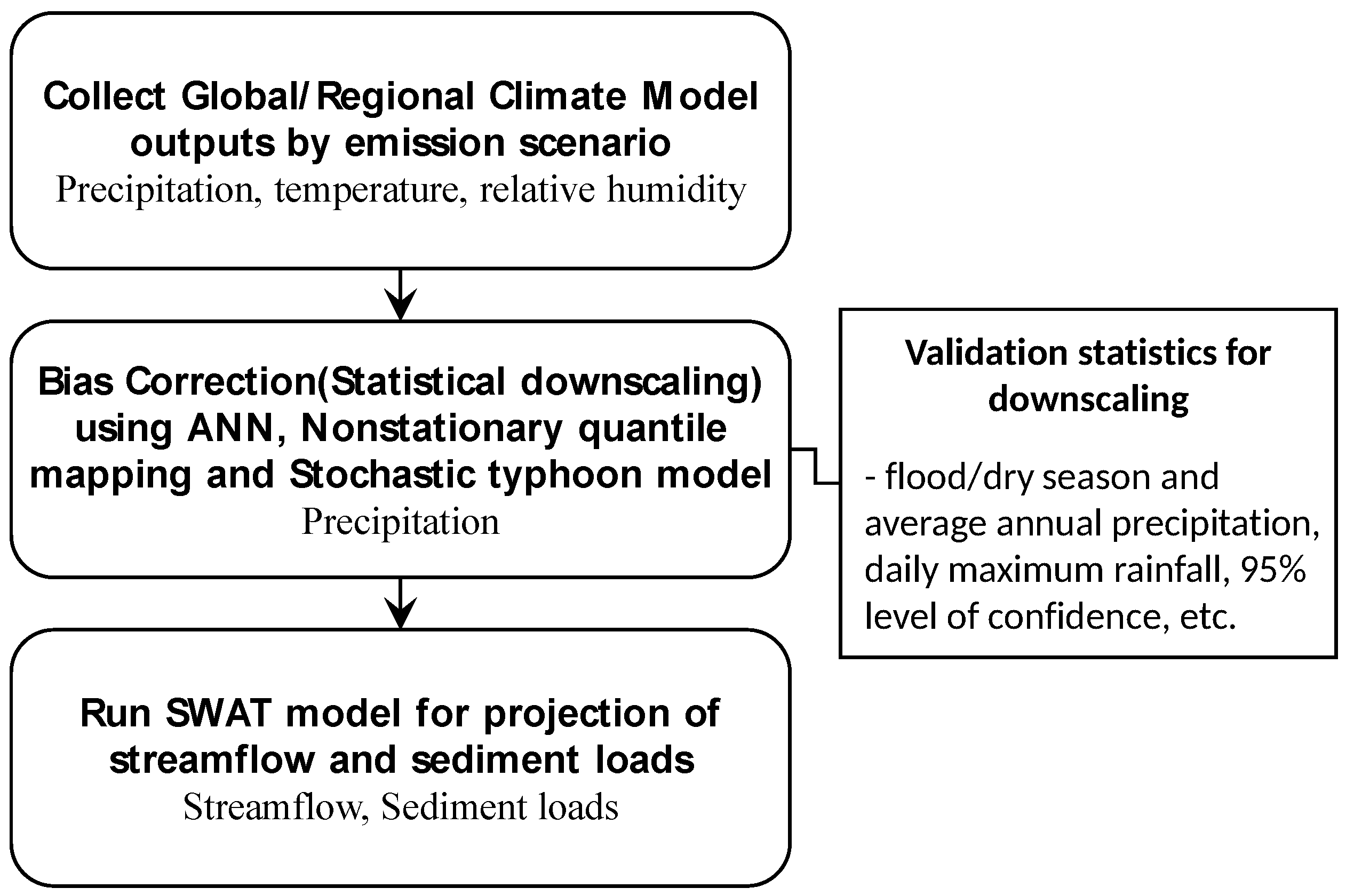
In this study, for the purpose of the reliable prediction of sediment yield in the watershed, the fine-scale projections for hydro-climate components were obtained first using the statistical bias correction and downscaling scheme based on the combination of ANN, Nonstationary Quantile Mapping (NSQM) and Stochastic Typhoon Synthesis (STS) sub-modules. Successively, the hydrologic runoff and sediment yield from the land surfaces were predicted through the long-term continuous watershed model, SWAT, using the bias-corrected and downscaled Regional Climate Model (RCM) output under the Intergovernmental Panel on Climate Change’s (IPCC’s) A1B climate change scenario.

2. Methodology

2.1. Framework of Regional Hydro-Climate Projection

The reliability of the projected climate change impacts depends largely on the quality of the climate change model output. The output of the RCM provided by the Korea Meteorological Administration (KMA) was used for the climate projection. The KMA’s RCM was developed by regionalizing the National Oceanic and Atmospheric Administration (NOAA’s) Mesoscale Model Version 5 (MM5) to the Korean climate environment. It downscales the ECHO-Gmodel output dynamically through the nested grid cascades from the ECHO-G to RCMs at a 12.5-km scale. The ECHO-G model consists of the atmosphere model ECHAM4and the ocean sea-ice model HOPE (Hamburg Ocean Primitive Equation), which incorporates a dynamic-thermodynamic sea-ice model with snow cover. The ECHAM4 has vertical 19 levels and a horizontal resolution of T30, corresponding to an approximate horizontal grid-point distance of 3.75 degrees. The performance of the T30/L19 version of ECHAM4 is described in Stendel and Roeckner [21]. The HOPE-G model used in ECHO-G is formulated on a Gaussian T42 Arakawa-Egrid corresponding to 2.8 degrees with grid refinement at low latitudes. The KMA’s RCM predictions have relatively finer-scale resolutions of 27 km compared to GCMs ($\simeq 400$ km) [22]. The modeling specifications for the global and regional models are compared in

Table 1. Specific information for the global and regional climate model provided by KMA.

	Global Climate Model (GCM)	Regional Climate Model (RCM)
Period	1860–2100 year	1971–2100 year
Scenarios	20C3M, A1B, B1, A2	A1B
Model output	ECHO-G	MM5
Grid scale	~400 km (~3.75°)	~27 km (~0.24°)
Grid information	87.157° S–87.159° N, 0°–360°	32.968° N–43.426° N, 122.935° E–131.447° E
Variables	Temperature (Max, Min, Average)	Temperature (Max, Min, Average)
	Precipitation, Relative Humidity	Precipitation, Relative Humidity
Data	Monthly	Monthly, Daily

. The RCM provides scenarios of five atmospheric variables; precipitable water, relative humidity, temperature (average, minimum, maximum) with daily-based 27-km spatial resolution under the IPCC’s Special Report on Emissions Scenarios (SRES) A1B of the AR4 scenario up to 2100. The overall procedure for this study is illustrated in Figure 1.

2.2. Study Area

The study area is the Hapcheon Dam basin located in the South Gyeongsang province, Korea, with an area of 928.9 km², a main stream length of 20.0 km and total reservoir capacity of 7.9 × 10⁸ m³. The average annual precipitation in the basin is 1324.3 mm for the period of 1991–2010. Among the stations in and around the basin, the Geochang station occupies 89% of the Thiessen coefficient and is treated as a representative station for hydro-meteorological data collection. The RCM precipitation used for an areal value for the Hapcheon dam basin was extracted from the nine grids surrounding Geochang station (Figure 2). The daily precipitation, temperature and relative humidity were extracted using the RCM from the Climate Change Information Center (CCIC) for the period of 1970–2100. Typhoons occur frequently from July–September both in frequency (1.43 occurrences on average for 1991–2010) and amount of rainfall (419.35 ± 251.0 mm), which is, in turn, the most vulnerable season with respect to the sediment detachment.

3. Statistical Downscaling: Overview

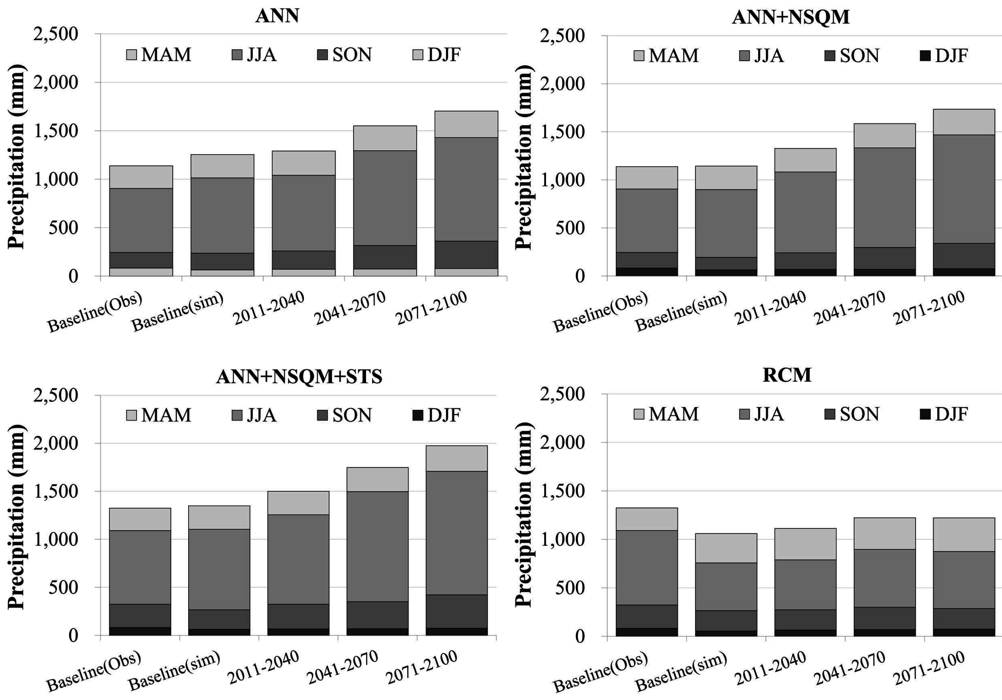
In order to produce the downscaled future projection of bias-corrected precipitation, a model chain of the ANN, NSQM and STS sub-modules was applied to the GCM precipitation output. The ANN is one of the Model Output Statistics (MOS) tools for correcting regional biases embedded in RCM or GCM [23,24]. The predictor variables for input to the ANN are precipitable water, relative humidity and temperature (average, minimum and maximum). In order to obtain improved modeling performance, the ANN structure was constructed separately for the flood (June–October) and non-flood (November–May) seasons. Additional data fitting was implemented with NSQM, which utilizes the temporally-varying statistical parameters reflecting the temporal trend captured by the original RCM and thus provides a more realistic projection with seamless connection with the baseline scenario fitted to the historical observation. The GCM or RCM does not include the local heavy rainfall and typhoon generation mechanism, which can be a reason for the underestimation of the summer precipitation [25]. Recently, Murakami et al. [26] developed a typhoon projection technique with high-resolution MRI-AGCMon a 20-km scale and applied it for an ensemble projection using the same model on a 60-km scale. However, the ensemble experiments with 60-km resolution MRI-AGCMs show large uncertainties in the projection of regional tropical cyclone changes. The developers claimed that future changes in the spatial distribution of Sea Surface Temperature (SST) are a major source of uncertainty in terms of future changes in the magnitude and frequency of tropical cyclones. 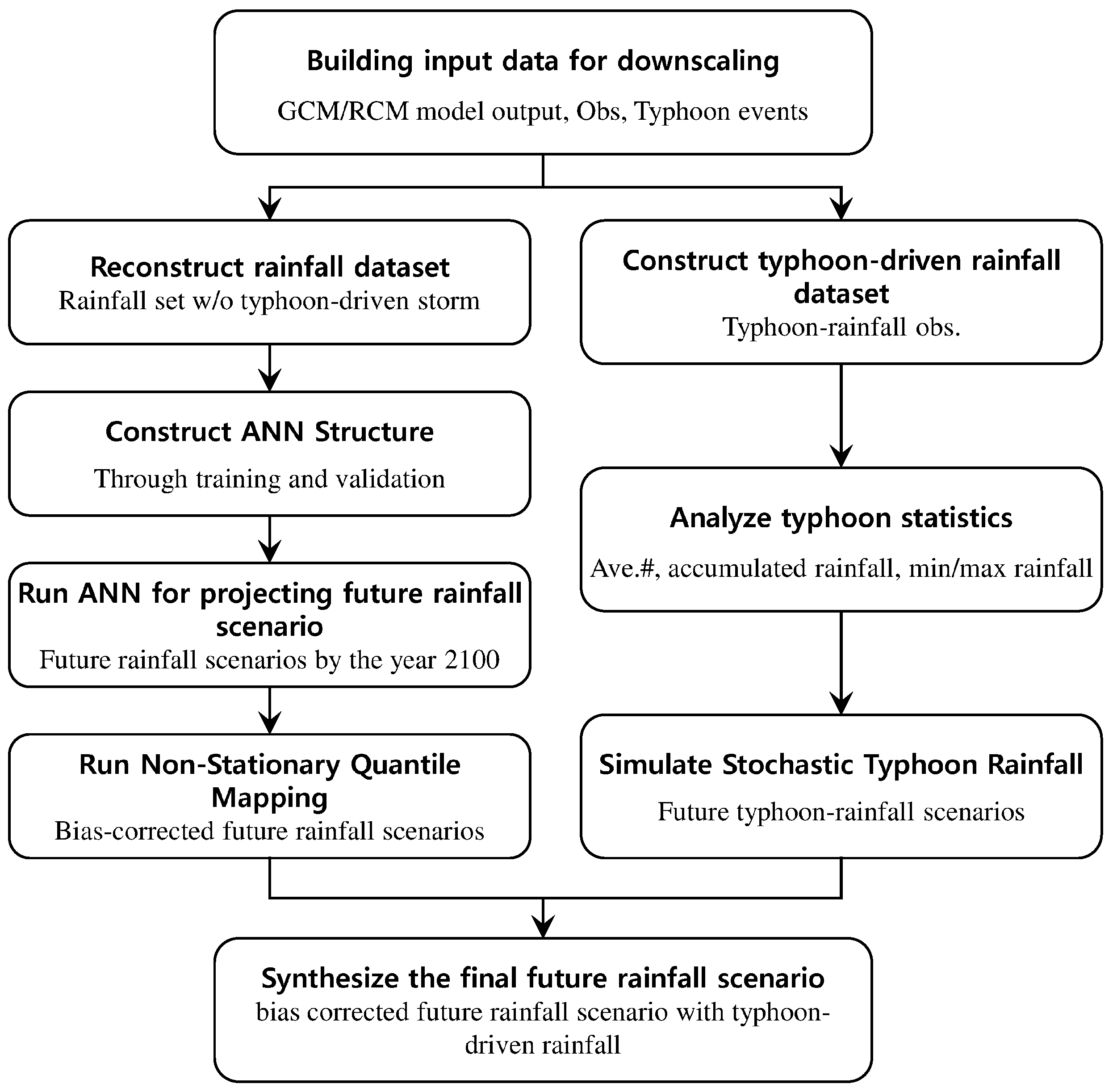The typhoon rainfall was simulated separately for the projection period, utilizing the STS sub-module, which generates the occurrence (and duration) and intensity of the typhoon using the mixed Poisson and Gumbel distribution, respectively [27]. In this study, in the process of producing the hydro-climate scenario with typhoon rainfall, the ANN training was carried out after eliminating the typhoon events that occurred during the flood season; the separately-simulated typhoon rainfall was then superimposed on the downscaled GCM output (Figure 3). The additional bias correction was implemented using the NSQM for the target probability density function with parameters varying consistently with the original GCM output. The periods of ANN training, validation and projection are 1991–2005, 2006–2010 and 2011–2100, respectively.

3.1. Statistical Downscaling: Artificial Neural Network Sub-Module

The ANN model is one of the popular nonlinear prediction models based on learning from the existing dataset. Applications of ANN in the atmospheric sciences have been reviewed by Gardner and Dorling [28] and others in the references for this current work. A number of additional research works have also been carried out in the areas of post-processing of numerical weather forecasting [24], precipitation forecasting [29], tornado warning [30], infilling missing daily weather records [31], weather forecasting [32], etc. Among them, Hall et al. [30]’s model was developed as part of the modernization of the National Weather Service (NWS) in the USA for the purpose of the local generation of Quantitative Precipitation Forecasts (QPFs) and their subsequent use in hydrological models at River Forecast Centers. Their model consists of two sub-networks of the Probability of Precipitation (PoP) network for the occurrence of precipitation and QPF for the amount of precipitation. As a daily network model for weather forecast, the PoP sub-network was necessary in advance of running the QPF model in order to enhance the model’s performance. However, the monthly ANN model outperformed the daily model because the random variability of the daily model is dominant over the periodic seasonal variation. In this study, the monthly ANN model was developed for downscaling the GCM precipitation output. Unlike the daily forecast model with its intermittent temporal occurrence, the monthly model allows the single module of QPF without the need to precede with the use of the PoP sub-module.

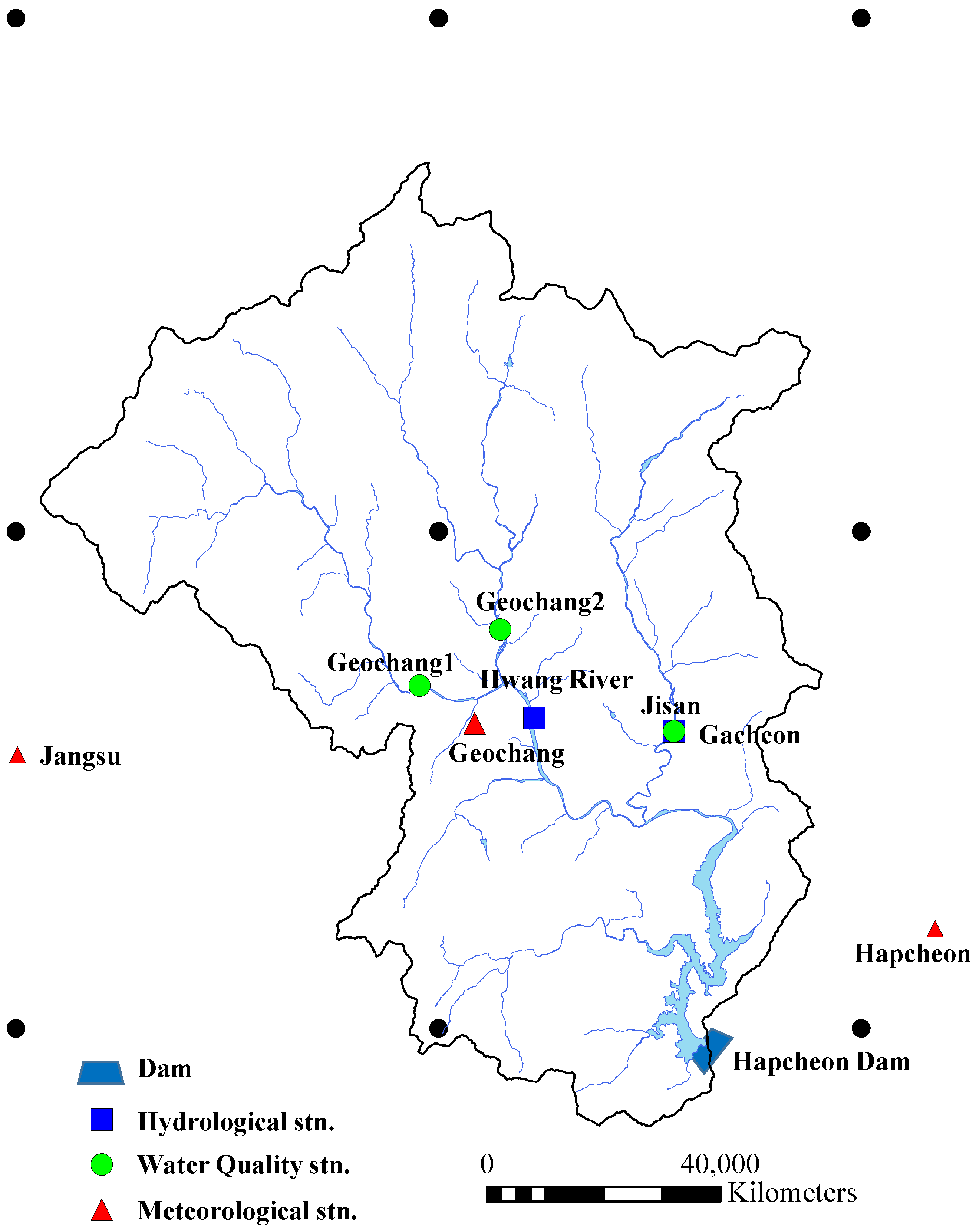
The QPF network was developed to predict monthly areal precipitation covering the Hapcheon dam basin area of 928.9 km² using the predictors of precipitable water, relative humidity and temperature (average, minimum, maximum) provided as the GCM output. The neural network has a three-layered feed-forward structure: signals flow forward from input layer neurons through any hidden units, eventually reaching the output neurons. Because the ANN scheme is a type of mapping for the weighted linear sum of predictor variables and the bias term through the activation function, the resulting output can appear as a negative value. The negative value can be avoided by, for example, taking a logarithm of the variables under consideration, if the hydrologic variables are positive values (i.e., precipitation or surface runoff). Prior to running the transformed neural network models, all of the inputs and outputs under consideration must be scaled to the network range bounded by the activation function. The activation function is usually selected to be a continuous and bounded nonlinear transfer function. The sigmoid function used in this study has the following form:

$$f\left(s_j\right)=\frac{1}{1+e^{-s_j}}$$

(1)

where $s_j\in [-\infty ,\infty ]$. Note that $f\left(s_j\right)$ is bounded on (0, 1).

The input layer consists of $n_I$ units, each of which receives one of the input variables. The so-called hidden layer is composed of $n_H$ units (i.e., neurons). Mathematically, a three-layer ANN can be written for each season as:

$$z_y\left(t\right)=\sum _{h=0}^{n_H}(w_h^{o}f(\sum _{i=0}^{n_I}(w_{hi}^h·z_x{\left(t\right)}_i-{\theta }_i))-{\theta }_h)$$

(2)

where:

• $z_x{\left(t\right)}_i$: the log-transformed input to unit i of the input layer
• $i=1,2,\cdots ,n_I$, where $n_I$: the number of inputs
• $h=1,2,\cdots ,n_H$, where $n_H$: the number of hidden units
• $w_{hi}^h$: the parameters, or weights, controlling the strength of the connection between the input unit i and the hidden unit h
• ${\theta }_i$ and ${\theta }_h$: the thresholds
• $w_h^o$: the parameters controlling the strength of the connection between the hidden unit h
• f: the activation or transfer function

3.2. Statistical Downscaling: Nonstationary Quantile Mapping Sub-Module

Most GCM and RCM generally show overall underestimation and regional biases, which should be restored or removed before being used for the impact model. Their ability to capture local/regional scale patterns of mean, variability, spatial-temporal correlation and extreme values that are directly relevant to the interests of the end users for hydrologic design and mitigation strategy planning is less promising, especially for precipitation (e.g., [33]). In general, the post-processing of bias correction can be classified into six methods, including the linear scaling, local intensity scaling, power transformation, variance scaling, distribution transfer and delta-change approach [34]. Among these methods, the distribution transfer method adjusts the systematic biases through mapping the Cumulative Distribution Function (CDF) of the model simulation into the target CDF of the observation or transformed observation [35], which is alternatively called “quantile mapping”, which is classified into the stationary and nonstationary parameter model.

$$\tilde{y}\left(t\right)=F_o^{-1}\left(F_m\left(y\left(t\right)\right|{\alpha }_m,{\beta }_m)\right|{\alpha }_o,{\beta }_o)$$

(3)

where F is the CDF of either the observations or the model. y(t) is the original value, and $\tilde{y}\left(t\right)$ is the bias-corrected value for a specific month (t).

The Gammadistribution [36] with shape parameter α and scale parameter β is often assumed to be suitable for distributions of precipitation events:

$$f(x;\alpha ,\beta )=\frac{x^{\alpha -1}{e}^{-x/\beta }}{{\beta }^{\alpha }\Gamma \left(\alpha \right)},x\ge 0,\alpha >0,\beta >0$$

(4)

where $\alpha ={\left(\frac{\overline{x}}{\sigma }\right)}^2$, $\beta =\frac{\overline{x}}{\alpha }=\frac{{\sigma }^2}{\overline{x}}$

3.3. Statistical Downscaling-Stochastic Typhoon Simulation Sub-Module

Generally, GCM and RCM are incapable of capturing the outbreak and development of a typhoon progressing at their sub-grid scale. In the calculated area affected hydrologically by the typhoon, the mathematically-generated typhoon rainfall should be included to meet the realistic total amount. In this study, the typhoon rainfall to be superimposed onto the downscaled GCM output was simulated for the projection period using the STS, which generates the occurrence (inter-arrival time) and magnitude of the typhoon rainfall using the mixed Poisson and Gumbel distribution, respectively (Moon, et al., 2012). The number of mean monthly typhoon occurrences during the flood season (June–October) was simulated using the Poisson distribution.

$$f(n_i;{\lambda }_i)=\frac{e^{-{\lambda }_i}{\lambda }_i^{n_i}}{n_i!},n_i=0,1,2,...,i=6,7,8,9,10$$

(5)

where:

• i: specific month (June–October)
• $n_i$: number of occurrences during the specific month
• ${\lambda }_i$: mean number of occurrences during the specific month

A number of research works have been carried out for the proper distribution of extreme precipitation events. The total amount, duration and intensities of tropical cyclone events showed typically skewed distributions of Gamma, Gumbel, Log-Pearson Type III, etc. [25,37,38]. The national probability map [39] of Korea was produced based on the Gumbel distribution, which was feasible for extreme storm events in most areas. The same distribution was adopted in “the guideline of design flood estimation [40]”. In this study, the Gumbel and its inverse function were applied using Equations (6) and (7). Assuming the temporal stationarity of the tropical cyclone during the projection period (2011–2100), the parameter of the monthly number of occurrences and the mean amount of rainfall for individual events were estimated using the year book on Korean tropical cyclones [41]. Using the uniformly-distributed random numbers and associated composite distributions, the monthly typhoon rainfall amounts were projected for the period of 2011–2100, preserving the stochastic performance during the past 20 years of the baseline period.

4. Hydrological Model

4.1. Continuous Long-Term Watershed Model: SWAT

The Soil and Water Assessment Tool (SWAT) model is a physically-based basin-wide continuous long-term yield model developed by the United States Department of Agriculture-Agricultural Research Service (USDA-ARS). It is a semi-distributed model with spatially-explicit parameterization and one of the most comprehensive models for simulating not only hydrologic runoff, but also water pollution load occurring from non-point sources in basins with complex terrains and varying soils, as well as varying land use and management. For this reason, SWAT is a popular model for the simulation of the hydro-environmental impacts of climate change. The surface runoff is estimated using the modified Soil Conservation Service (SCS) curve number method [42], which enables adjustment of effective runoff at each time step based on the amount of soil water present. The Green–Ampt method is another option, but is not applicable in this study because it requires sub-daily rainfall data.

Data for the topography, land use and management, soils and weather data required to derive the SWAT input parameter values were compiled using databases managed by various governmental agencies. The elevations, land use and stream network data were obtained from the Ministry of Land, Infrastructure and Transport’s (MOLIT’s) Water Resources Management Information System (WAMIS). It includes data from the 30-m resolution Digital Elevation Models (DEMs) digitized from a 1:5000 contour map of the National Geographic Information System (NGIS), stream network data and quadrangles of land use/land cover data with the same scale (Figure 4).

Soil properties were extracted from a 1:25,000 detailed soil survey geographic database provided by the Korea National Academy of Agricultural Science (NAAS). Daily precipitation and minimum and maximum temperatures for the Geochang station in the study area were retrieved from WAMIS. The data format and sources for the meteorological and environmental data are listed in

Table 2. Meteorological and environmental data.

Category		Components	Source
	Surface runoff	Daily mean surface runoff	Kwater
	Precipitation	Daily precipitation (mm)
Meteorology	Temperature	Daily max. temp. (°C)	KMA
	Solar radiation	Daily solar radiation (MJ/m${}^2$)
	Wind speed	Daily mean wind speed (m/s)
	Relative humidity	Daily mean relative humidity (%)
Water quality	Point pollution source	Elementary Environmental Facilities	Ministry of
	Sediment	Monthly sediment (ton)	Environment

. Each sub-watershed is divided into one or several homogeneous Hydrological Response Units (HRU) obtained by overlying the soil and land use maps. The response of each HRU in terms of water, sediment and nutrient losses is then aggregated at the sub-basin level and routed to the watershed outlet through the channel network.

In SWAT, the HRU-level erosion caused by rainfall and runoff is computed using the Modified Universal Soil Loss Equation (MUSLE). In MUSLE, the rainfall energy factor is replaced with a runoff energy factor that is closely correlated with the amount of detached and transported sediment [43]. The sediment yield estimated for each HRU is improved such that runoff becomes a function of the antecedent moisture condition, as well as rainfall energy.

$$Q_s=11.8{(Q\times q_p\times A)}^{0.56}\times K\times C\times P\times LS\times CFRG$$

(6)

where $Q_s$ = the sediment yield on a given day (ton), Q = the surface runoff volume (mm/ha), $q_p$ = the peak runoff rate (m${}^3$/s), A = the area of the HRU (ha), K = the Universal Soil Loss Equation (USLE) soil erodibility factor, C = the USLE cover and management factor, P = the USLE support practice factor, $LS$ = the USLE topographic factor and $CFRG$ = the coarse fragment.

The sediment routing in the channel [44] consists of channel degradation using stream power and deposition in the channel using fall velocity. Channel degradation is adjusted using the USLE soil erodibility and channel cover factors [45]. MUSLE has been widely used in many locations and applications throughout the world. However, it has been pointed out that MUSLE overestimates the sediment yield from rangelands and underestimates those from croplands [46]. Additionally, Strauss and Klaghofer [47] found that MUSLE overestimated soil loss in areas with high erosion risk and underestimated it in areas with low erosion risk.

4.2. SWAT Calibration and Validation (Surface Runoff and Sediment)

There is no single accepted statistic or test that determines whether or not a model is valid. Furthermore, it is hard to assess the priority among performance indices. Simply the model validation comparison can be made in terms of point-to-point paired data performance, time and/or space integrated paired data performance, frequency domain performance, etc. The acceptable range of the performance indices is suggested in

Table 3. Performance indices and the feasible range by hydrologic components.

Components	Performance Index	Feasible Range
Surface Runoff	d (%) *	≤15
	R${}^2$ **	≥0.6
	COE ***	≥0.5
Total Flow	d (%)	≤15
	R${}^2$	≥0.6
	COE	≥0.5
Sediment	d (%)	≤20
	R${}^2$	≥0.6
	COE	≥0.5
Nutrient	d (%)	≤20
	R${}^2$	≥0.6
	COE	≥0.5

Notes: * d: Percent difference between measured and simulated average daily values; ** R${}^2$: Coefficient of determination; *** COE: Nash–Sutcliffe efficiency coefficient.

.

A variety of parameters are to be calibrated in the SWAT model. The default, calibrated and feasible range of the underlying parameters are summarized in

Table 4. Calibrated parameter values.

Parameter	Default Value	Calibrated Value	Feasible Range
Groundwater delay	31	80	0–500
(GW-DELAY (days))
Base flow alpha factor	0.048	0.15	0–1
(ALPHA-BF (days))
Groundwater revapcoefficient	0.02	0.2	0.02–0.2
(GW-REVAP)
Deep aquifer percolation fraction	0.05	0	0–1
(RCHRG-DP)
Manning’s n value for overland flow	0.1	0.013	0.01–30
(OV-N)
Soil evaporation compensation factor	0	0.5	0–1
(ESCO)
Initial SCS runoff curve number for Moisture Condition II	67	47	35–98
(CN2)
Moist bulk density	1.61	0.9	0.9–2.5
(SOL-BD (g/cm${}^3$))
Available water capacity of the soil layer	0.15	0.4	0–1
(SOL-AWC (mm/mm))
Saturated hydraulic conductivity	43.15	20	0–2000
(SOL-K (mm/h))

.

Multi-site calibration was carried out using daily surface runoff data at upstream sites (Hwang River and Jisan) and the outlet of the Hapcheon dam basin. The warm-up period was established as the initial two years (2002–2003) for computational stabilization. The calibration and validation periods were set as 2004–2005 and 2006–2007, respectively. The land use and soil properties of the watershed were left unchanged throughout the simulation period. Potential Evapotranspiration (PET) was computed through the widely-used Penman–Monteith method. Additionally, the Muskingum routing method is adopted for channel routing. In this study, model calibration was performed by trial and error, in order to maximize the objective function of R${}^2$, the Nash and Sutcliffe coefficient (NSE) and the Root Mean Square Error (RMSE), in addition to the good adjustment of the simulated hydrograph compared to the baseline. Like most daily continuous rainfall-runoff models, accurate calibration for both high and low flows is not easily accomplished. Fitting suspended sediments requires rainfall with a high intensity at the sub-daily scale. Available water quality measurements show the weekly to monthly periods of measurement, while the allowable range of calibration was set in advance.

The basin runoff was computed as the volumetric surface runoff or dam inflow divided by the upstream basin area. The runoff calibration for the Hapcheon Dam basin was implemented first at the upstream gauging stations of the Hwang River and Jisan sites and then subsequently at the basin outlet of the dam site. During the calibration and validation periods, the annual average surface runoff shows a performance of R${}^2$ = 0.82, NSE = 0.77, RMSE = 0.94 mm/day and R${}^2$ = 0.80, NSE = 0.78, RMSE = 3.16 mm/day at the Hwang River and Jisan stations, respectively. In addition, the Hapcheon dam outlet shows the performance of R${}^2$ = 0.78, NSE = 0.76, RMSE = 3.80 mm/day during the same period. The simulated runoff was underestimated by 25% on average, which is interpreted as a limitation of the daily continuous rainfall-runoff model, and additional calibration was not carried out in order to avoid an unrealistic range of parameters (Figure 5 and

Table 5. Performance of the rainfall-runoff model calibration and validation at the Hapcheon dam site.

Modeling	Year	Precipitation	Surface Runoff (mm)		Runoff Ratio (%)		R2	NSE	RMSE
Period		(mm)	(Obs)	(Sim)	(Obs)	(Sim)
Calibration	2004	1547.2	1122.4	867.7	72.5	56.1	0.74	0.70	5.32
	2005	1245.3	850.1	643.1	68.3	51.6	0.72	0.70	3.19
Validation	2006	1411.8	968.6	756.4	68.6	53.6	0.94	0.93	1.92
	2007	1729.5	1282.4	900.9	74.1	52.1	0.74	0.72	4.80
Mean		1483.4	1055.9	792.0	70.9	53.3	0.78	0.76	3.80

).

Following the calibration and validation of surface runoff, basin-wide water quality calibration was carried out at the general water quality sites of the Geochang 1, 2 and Gacheon stations and the Total Maximum Daily Loads (TMDL) site of Hwang River Station “A” immediately upstream of the dam reservoir. The water quality data are available at the Water Information System (WIS) managed by the National Institute of Environmental Research (NIER) who are operating the national water quality monitoring network for the TMDL policy. Unlike surface runoff, the sediment yield involves a complex procedure, including detachment from land surfaces, transport and deposit, and is simulated mostly using empirical equations. While precipitation is definitely the major driving force for triggering the sediment process, a lack of understanding of the holistic physical processes remains. Moreover, the available continuous measuring dataset is mostly limited. Even NIER’s national TMDL monitoring network provides sediment observation data with eight-day intervals. Consequently, the simulated results can involve a large number of uncertainties and need careful consideration in dealing with discrete observation data in comparison with continuous simulation data for data interpretation and model calibration. Figure 6 compares the monthly observation and simulation of the sediment yield at Hwang River station “A” and Jisan station. The daily simulated results show a high degree of daily fluctuation noise, which hinders direct date-to-date comparison with observations of eight-day intervals. The results of monthly accumulated sediment yield have the advantage of capturing temporally long-term behavior. At Gacheon station, the simulated sediment yields during both high and low flow regimes are captured with a relatively similar temporal pattern with observation. However, at the Hwang River station “A”, the simulated capability in the high flow regime is not sufficiently validated, which is interpreted as the limitation of the model using the daily rainfall intensity value. The sediment yield at the Hapcheon Dam site was computed using the values at the Hwang River “A”, the Jisan site and the areal multiplication factor. Because the Hapcheon Dam site is the outlet of the water quality monitoring network, the accurate calibration for sediment yield would have a limitation.

5. Projection Results

5.1. Precipitation

The ANN structure is determined through training with the predictors and predictand dataset during the baseline period. Using the trained and validated ANN model, the precipitation, relative humidity and the maximum and minimum temperatures during future periods until 2100 are projected using the GCM model output during the projection period. For the purpose of improving the training performance, the neural network training was performed separately for the flood (June–October) and non-flood (November–May) seasons. Finally, the improved ANN structure, superior to the original RCM climate components, is determined through the correlation coefficient and analysis of error.

In particular, the precipitation was performed to compare with step-by-step results of downscaling under the A1B scenario for checking the improvement of the composite ANN method compared to the single ANN method. The typhoon rainfall was excluded in the dataset for training and validating ANN and NSQM in order to enhance the modeling performance during the flood season. The available model output of one complete set of 100-year daily data and three groups of projection scenarios for the following 30-year periods included the following: the Foreseeable Future Scenario (FFS) (2011–2040), the Mid-term Future Scenario (MFS) (2041–2070) and the Long-term Future Scenario (LFS) (2071–2100).

The seasonal projection results from RCM and the sequential additive combination of the downscaling, bias-correction and stochastic typhoon models are compared in Figure 7. The raw RCM output shows the overall underestimation and −20.0% bias from the observation during the baseline period. Through all combined downscaling processes, the biases were removed, and the coupled ANN-NSQM and ANN-NSQM-STS exhibit only 0.5% and 1.9% biases, respectively (

Table 6. Rate of projected precipitation increase by stages of composite downscaling modules.

Downscaling Schemes	Baseline	Baseline	2011–2040	2041–2070	2071–2100
	(Obs)	(Sim)	(FFS)	(MFS)	(LFS)
RCM	1324.3	1059.8	1112.8	1223.0	1221.4
		(−20.0) **	(5.0) ***	(15.4) ***	(15.2) ***
ANN	1137.5 *	1253.7	1290.6	1550.3	1702.5
		(10.2) **	(2.9) ***	(23.7) ***	(35.8) ***
ANN + NSQM	1137.5 *	1143.8	1327.2	1584.1	1735.1
		(0.5) **	(16) ***	(38.5) ***	(51.7) ***
ANN + NSQM + STS	1324.3	1349.8	1500.5	1747.3	1974.6
		(1.9) **	(11.2) ***	(29.4) ***	(46.3) ***

Notes: * Annual precipitation without typhoon; ** ratio of baseline (Sim) vs. baseline (Obs); *** ratio of projections vs. baseline (Sim) by projection future.

). The addition of the stochastic typhoon model restores the underestimated raw climate model output. Under the A1B scenario, 16.4% and 13.8% of annual precipitation were restored during the baseline period and long-term future period (2071–2100). The projection for annual precipitation shows a 25.7% and 57.2% increase with respect to the baseline period by 2040 and 2100, respectively. The increasing rate (33.4% and 72.5%) during the flood season is much higher than that for the annual total amount. The range of variability increases with time. The upper and lower limits of a 95% confidence interval with respect to the annual mean value are ±25.6% and ±32.1% in 2040 and 2100. The variability range for the flood season is ±32.4% and ±39.7% in 2040 and 2100, respectively, which is higher than the rates for the entire season, similar to the mean statistics. The variability and rate of change for the non-flood season stays relatively weak during the projection period (Figure 8).

The maximum daily precipitation is more closely connected to the sediment processes on the terrestrial land surface than to the long-term annual precipitation because long-term sediment yield is obtained from the accumulation of a large number of isolated erosion events with a daily or sub-daily time scale (Michael et al., 2005). The basic idea involves rearranging the time series of the raw RCM daily projection data, such that their daily biases are corrected proportionally to the ratio between the raw and downscaled monthly RCM output using Equation (7). The ANN-based downscaling was carried out for the monthly data rescaled from the raw daily RCM output for the purpose of raising network training performance. In 2100, the maximum daily precipitation is expected to reach 127.6 mm/day, which is a 54.4% (= 44.9 mm/day) increase with respect to the baseline period (Figure 9).

$$P_{RCM\_day}^{\prime }=P_{RCM\_day}\times \frac{P_{ANN\_mon}}{P_{RCM\_mon}}$$

(7)

5.2. Surface Runoff and Hydrologic Components

The future projection of basin-wide runoff and variation of hydrologic components was implemented through the SWAT model using the downscaled daily RCM output under the IPCC’s A1B climate change scenario. The land use and vegetation conditions were assumed to be stationary during the projection period. In the foreseeable future (2011–2040) and long-term future (2071–2100), the annual dam inflows are expected to increase by 15.8% and 63.2%, respectively. Monthly dam inflow variation exhibits relatively higher increasing trends in the future, particularly in the JJA and September, October, November (SON) seasons with not only an increasing ratio (19.5% and 73.8% during the FFS and LFS periods, respectively), but also an increasing absolute value (Figure 10).

Along with the surface runoff, the hydrologic components of dam inflow, direct runoff, base flow and evapotranspiration at the basin outlet were projected together through the SWAT model. The two-way interaction between hydrologic components, e.g., the physics of energy and mass transfer at the land surface-atmosphere interface and the resulting regional weather variations, are very complicated, and our understanding is still limited [48]. In this study, the SWAT model computes the hydrologic components simply based on the assumption of stationarity in precipitation loss from evapotranspiration and infiltration during the projection period and disregards the interaction between regional precipitation and evapotranspiration and its impacts on the effective precipitation and resulting surface runoff. Figure 11 shows that the direct runoff increases 1.52-times more than precipitation. The higher increasing ratio of direct runoff compared to precipitation provides a noticeable warning for water resource managers to build a strategic plan for adapting to climate change. In terms of mass balance between precipitation and runoff, the result was beyond that expected and can be explained by the fact that only part of the total precipitation flows into a dam, i.e., the runoff coefficient of 66.1% during the projection period and the assumption of stationary precipitation loss.

The evapotranspiration in the figure is potential evapotranspiration computed through the Penman–Monteith equation in which the PET is the function of solar radiation, air temperature, relative humidity and wind speed. According to the complementary relationship suggested by Bouchet [49], PET is negatively proportional to available moisture (precipitation) under the fixed condition of ambient temperature. However, if moisture supply (precipitation) is fixed, PET increases with temperature, because atmospheric demand for moisture increases under high temperature. Thereby, the PET can keep constant as the net result of increase in precipitation and temperature, even though it can vary spatially and temporally.

5.3. Flow Regime (Flow-Duration Curve)

The future variation of the flow regime was assessed from the flow duration curve, which gives the flow rate with various percentiles of Q95 (high flow), Q185 (normal flow), Q275 (low flow) and Q355 (drought flow). The only high flow exhibits an obvious increasing trend of an 11.5 m${}^3$/s (40.7%) increase during the projection period (Figure 12). Along with the trend of daily maximum precipitation, it is an essential clue for the future increase of sediment yield. The Coefficient Of River Regime (CORR) illustrates indirectly the vulnerability of the river against sediment scouring during the flood season. The CORR is computed as the ratio between Qmax and Qmin. During the long-term future period, CORR reaches 353.9 (27.2% increase with respect to the baseline). To avoid the over-estimation due to the data regarding extreme flood and drought events, the Coefficient Of Flow Duration (COFD), which is the ratio between Q10 and Q355, is alternatively used. The COFD also increases 22.6% during the long-term future period (

Table 7. Projections for coefficient of river regime and flow duration by three decadal spans.

	1990–2010	2011–2040	2041–2070	2071–2100
	(Baseline)	(FFS)	(MFS)	(LFS)
Coefficient of River Regime	278.3	239.6 (−13.9%)	294.5 (5.8%)	353.9 (27.2%)
Coefficient of Flow Duration	75.2	69.9 (−7.0%)	79.3 (5.4%)	92.2 (22.6%)

).

5.4. Sediment Yield

Similar to the surface runoff component, the future projection of the sediment yield was computed through the SWAT model using the downscaled daily RCM output under the same scenario. The change in precipitation intensity and associated hydrologic components has a direct impact on sediment yield and other water quality loads from non-point sources. The overall variation pattern of sediment yield is proportional to the basin-wide surface runoff. The annual sediment yield shows 27.4% and 121.2% increases during the foreseeable and long-term future periods, respectively. The JJA season of LFS occupies 83.0% annual total sediment yield during the baseline period, which is similar during the projection period (

Table 8. Monthly projection of sediment by periods at Hapcheon Dam basin.

		1990–2010	2011–2040		2041–2070		2071–2100
		Sediment (ton)	Sediment (ton)	Change (%)	Sediment (ton)	Change (%)	Sediment (ton)	Change (%)
	December	43.4	103.1	137.7	106.1	144.7	149.5	245.0
DJF	January	22.8	42.2	84.8	70.0	206.3	76.5	234.7
	February	15.2	29.9	96.6	28.4	86.6	52.9	247.5
	March	27.7	35.9	29.8	67.3	143.2	66.2	139.0
MAM	April	301.3	533.9	77.2	693.9	130.3	885.9	194.1
	May	2106.7	2104.8	−0.1	2129.7	1.1	2346.1	11.4
	June	5569.2	10,508.9	88.7	13,151.2	136.1	18,041.8	224.0
JJA	July	23,847.3	27,436.9	15.1	41,763.4	75.1	47,955.2	101.1
	August	21,688.2	25,693.8	18.5	35,757.4	64.9	46,505.6	114.4
	September	7613.4	11,510.3	51.2	12,421.6	63.2	17,781.2	133.6
SON	October	135.7	289.9	113.7	400.3	195.1	1616.3	1091.4
	November	178.9	150.7	−15.8	441.7	146.9	698.9	290.5
Annual		61,549.8	78,440.3	27.4	10,7031.1	73.9	136,176.0	121.2

, Figure 13).

Even though October shows the highest increasing ratio of 1091.4%, its absolute value is only 8% of the annual total. During the baseline period, the sediments in October comprise 1.7% of the annual total, which is much lower than that of the long-term future. Figure 14 shows that the relative change of sediment yields is 1.9-times higher than that of the dam inflows.

Uncertainty is one of the key issues in climate change impact projection. In particular, it would be more critical in the projection with the coupled model chain. The uncertainties of hydro-climatic components propagate or are amplified along the model chain from the climate model output to the sediment runoff model. Ensemble and Monte Carlo approaches [50,51] are schemes for representing the range of reliability for the variables of interest. Using different time series allows estimating the uncertainty of the model in terms of precipitation. However, the statistical way to realize uncertainty does not give a clue to trace the uncertainty embedded in the rainfall-sediment runoff modeling. The temporal scale of rainfall is critical according to the objectives of the sediment projection for sediment deposition or wash load. Accurate modeling for coarse particles requires rainfall of high intensity with a sub-daily scale. In sediment projection, the temporal disaggregation to the sub-daily scale is theoretically desirable, but does not give always reliable results. For example, SWAT requires Green–Ampt modeling or a new mixed modeling [52] option for infiltration when using sub-daily rainfall, but a bit more additional information, e.g., Moisture Condition II curve number, saturated hydraulic conductivity of surface layer, moist bulk density, % clay content, % sand content, etc., for Green–Ampt modeling.

6. Conclusions

The hydro-environmental impact in the context of sediment yield associated with basin runoff was evaluated using the SWAT model under IPCC’s climate change scenario. The precipitation projection was based on the RCM MM5 model output under the AR4 A1B scenario and was downscaled statistically using the combination of ANN, nonstationary quantile mapping and the stochastic typhoon simulation model. Through separating the typhoon rainfall out and the use of the monthly accumulated rainfall for training and validation, the performance of ANN modeling could be improved. In order to reproduce the temporally-varying trend reflecting climate change, quantile mapping with temporally-varying parameters of the target distribution was applied. Considering that realistic simulation of sediment yield is closely related to the rainfall event with high intensity and frequency, the typhoon rainfall was simulated separately. The incremental improvement of the combined downscaling process was evaluated successfully during the baseline period, which provides projected confidence for the simulated future scenario.

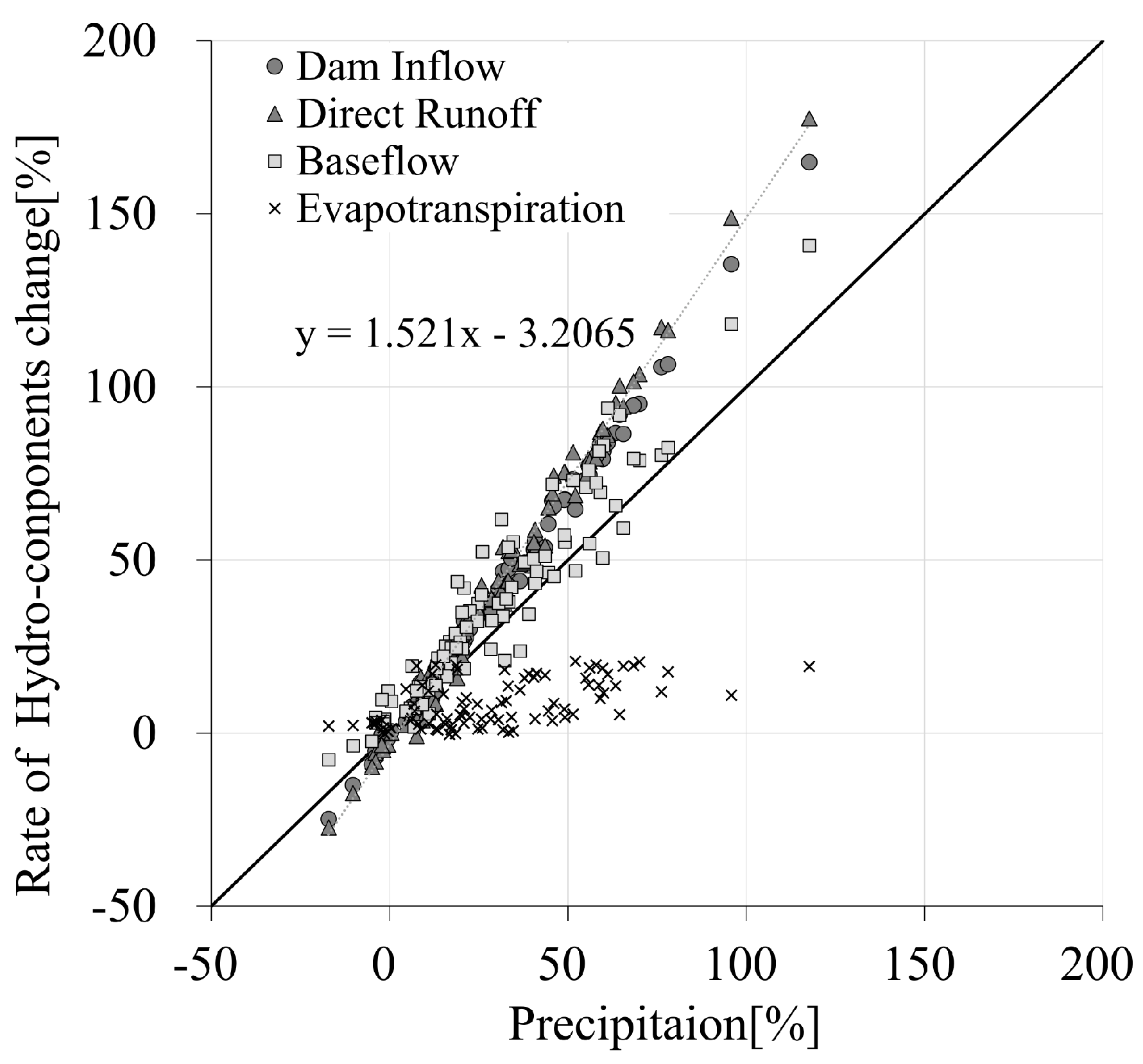
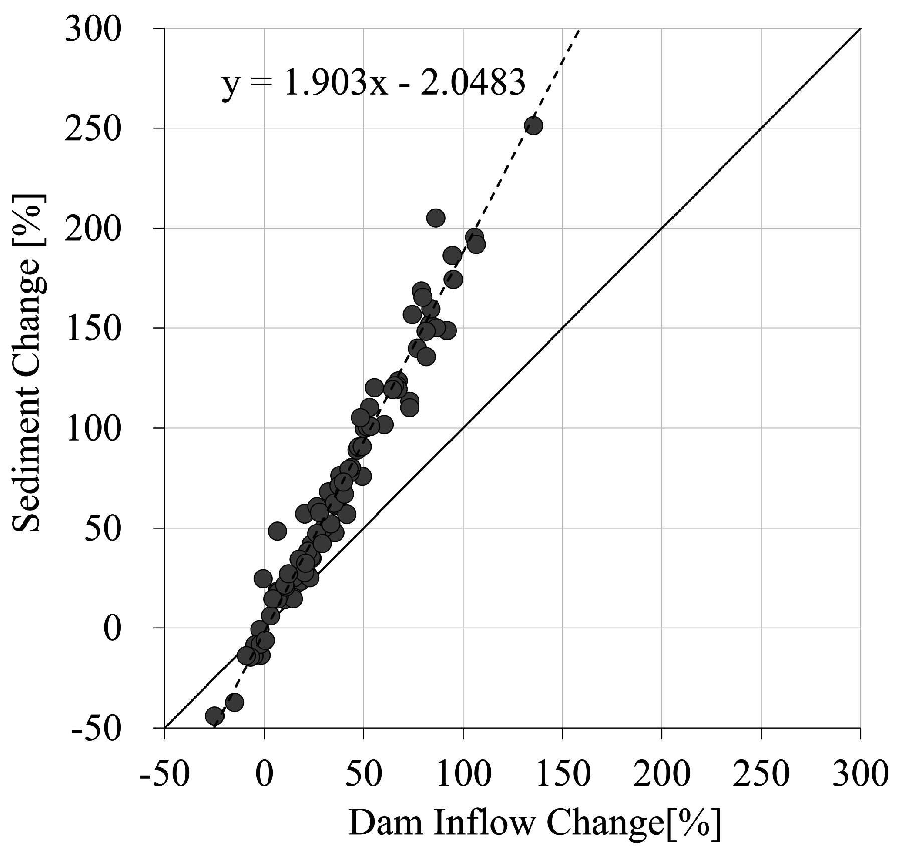
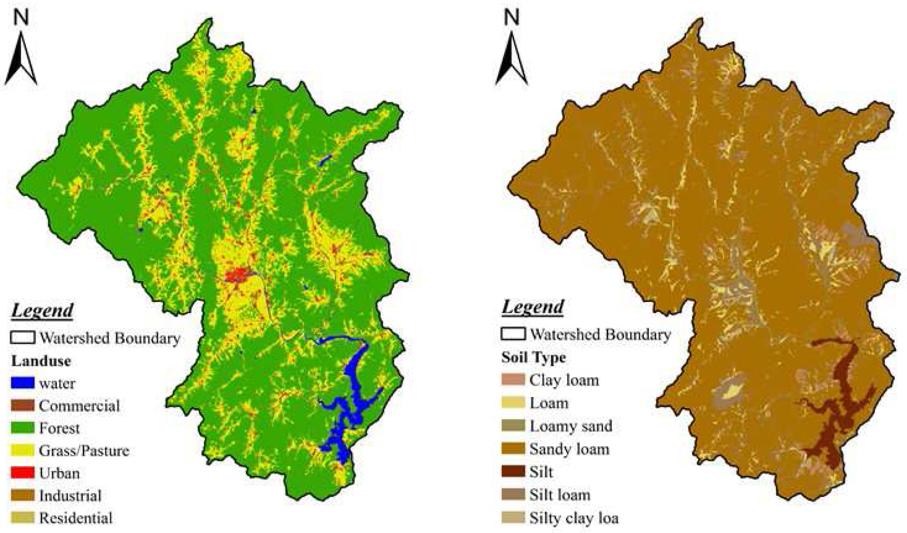
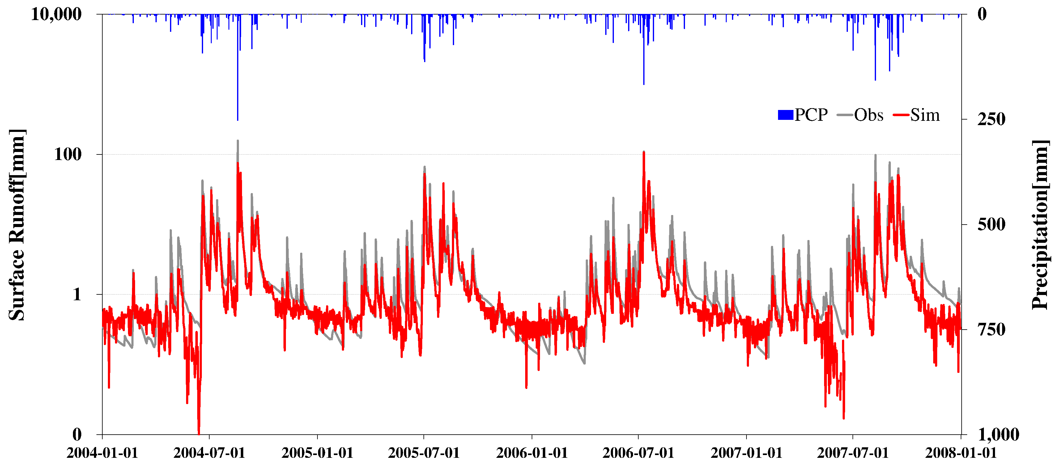
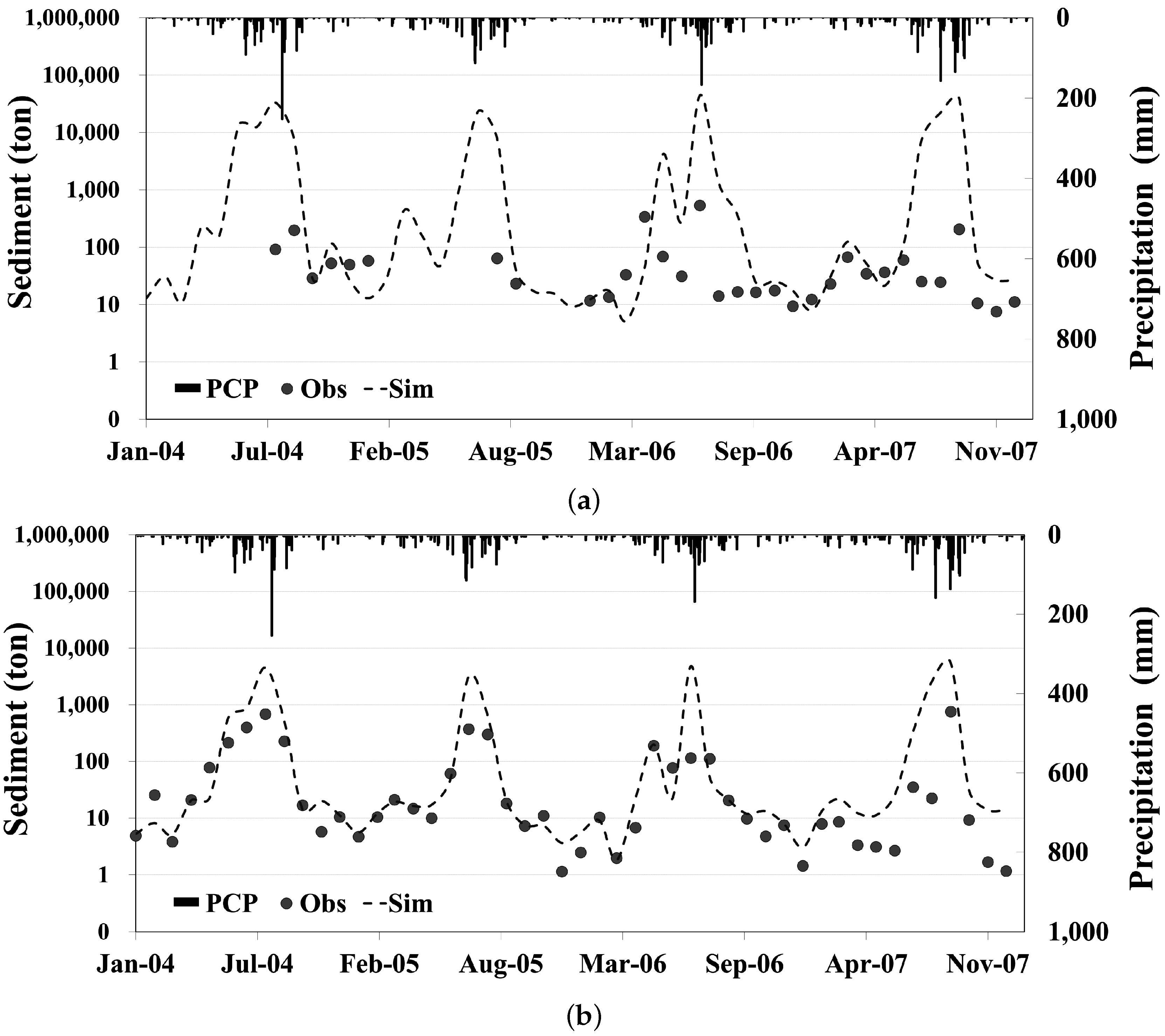
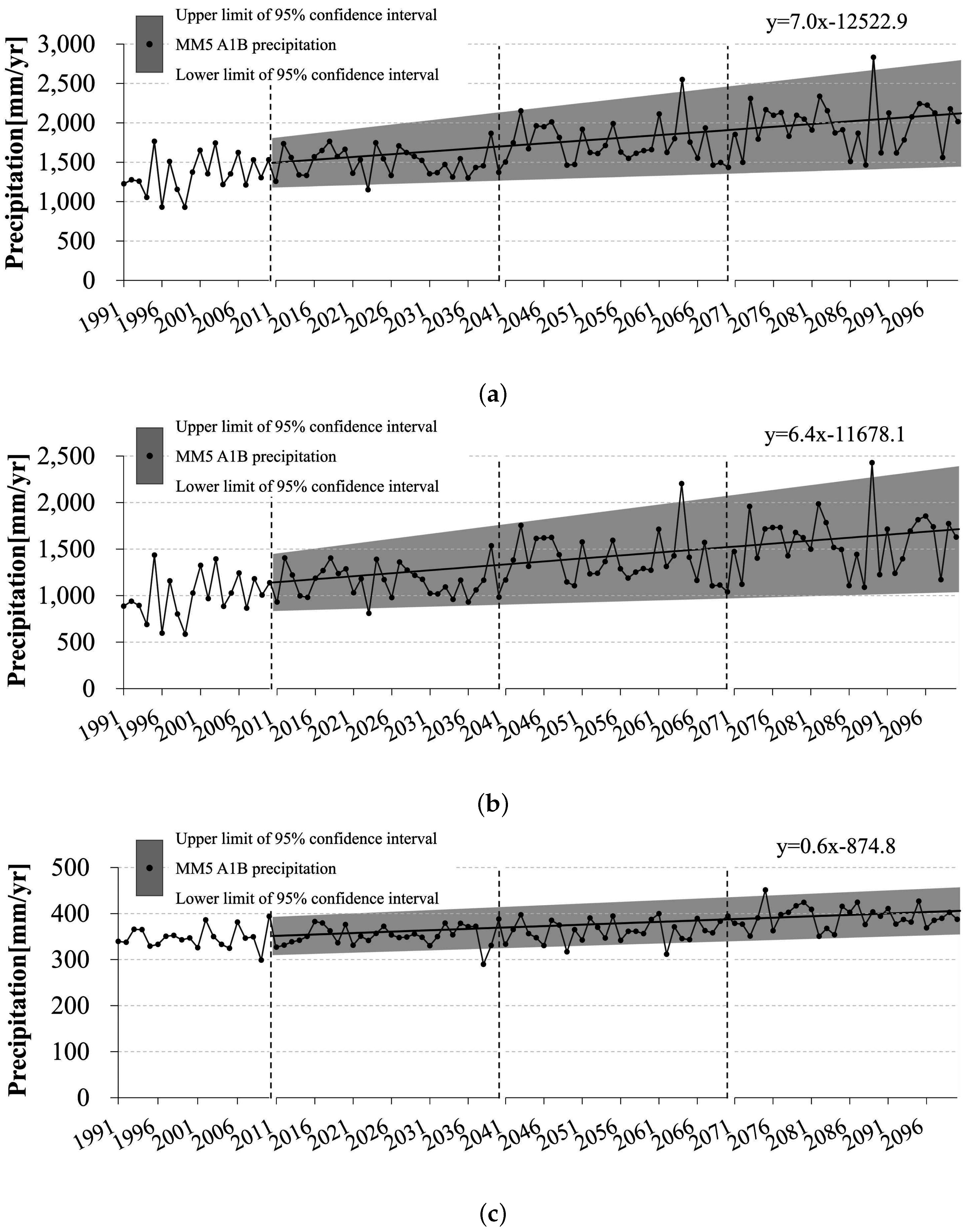
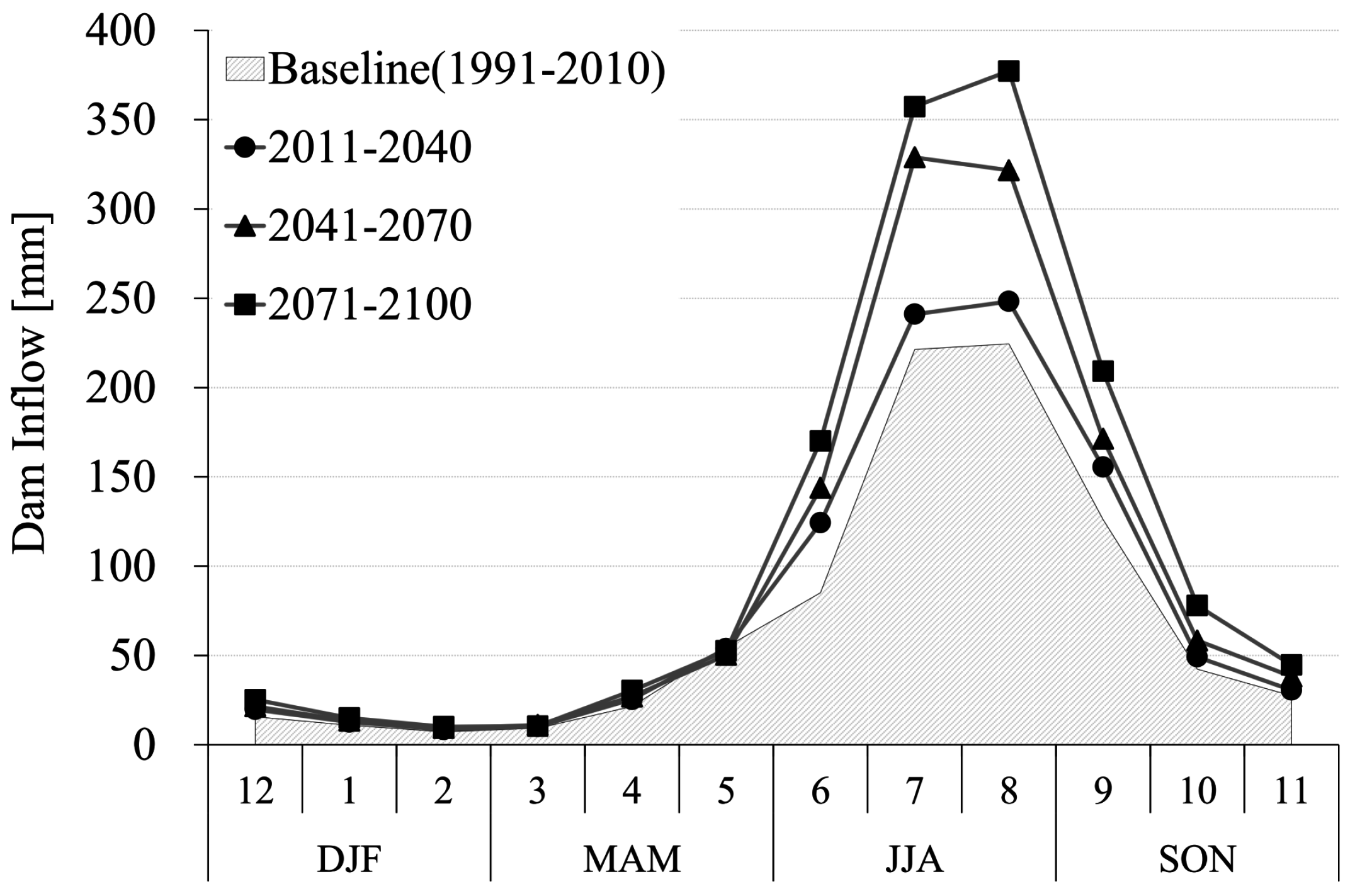
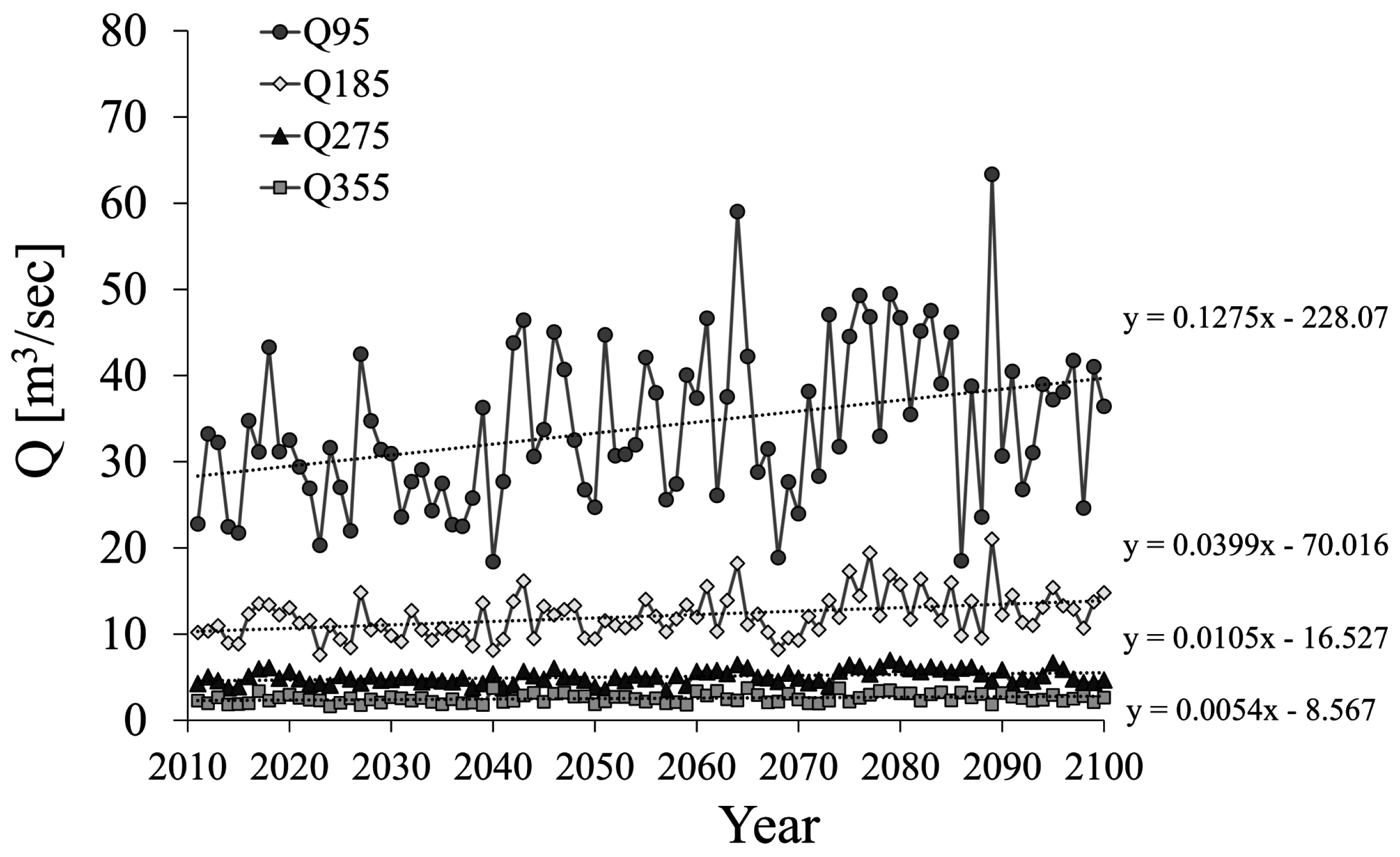
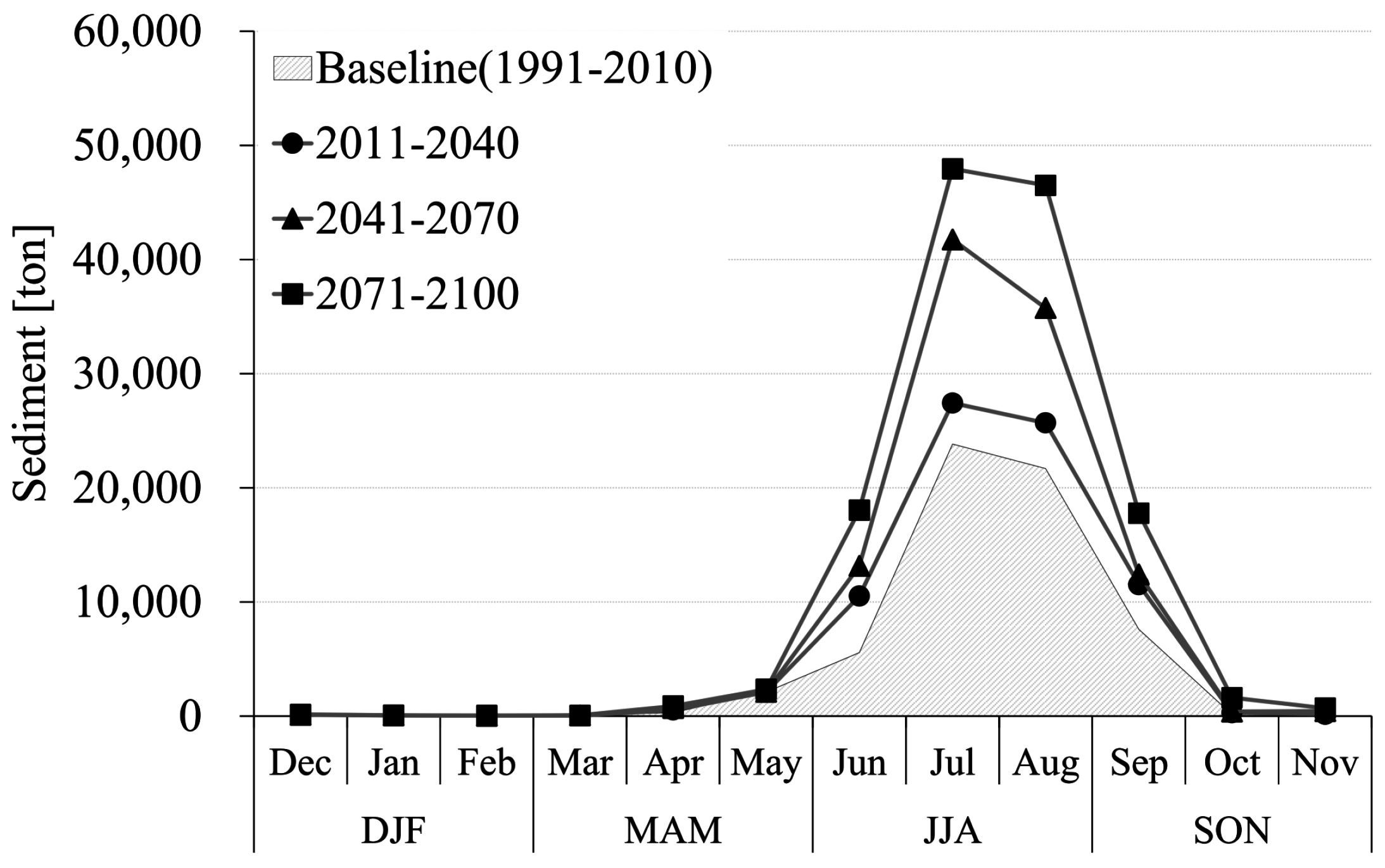
The basin scale long-term runoff and sediment yield according to various soil and land use types were computed using the physically-based semi-distributed continuous rainfall-runoff model, SWAT. The calibration was implemented sequentially from the HRUs in the upstream area to the basin outlet. From a practical point of view, the water quality monitoring network has a lack of density, observation cycle and available periods, which renders reliable calibration and validation of sediment yield difficult. Accordingly, the modeling performance was evaluated for the monthly accumulated amount rather than using a comparison of the directly continuous daily simulations with the eight-day interval observations. The biases possibly occurred because the surface runoff gauging station and the water quality monitoring station are located apart. The biases were corrected considering the area correction factor. The ANN modeling was implemented separately for the flood (June–October) and non-flood (November–May) seasons. The training, validation and projection were carried out during the periods of 1991–2005, 2006–2010 and 2011–2100, respectively. The projection results were illustrated for 30-year periods of FFS (2011–2040), MFS (2041–2070) and LFS (2071–2100). The land use and vegetation changes during the projection periods were not considered. The projection for annual precipitation shows 25.7% and 57.2% increases with respect to the baseline period by 2040 and 2100, respectively. In particular, the increasing rate (33.4% and 72.5%) during the flood season is much higher than that for the annual total amount. However, the sediment yield is expected to increase by 27.4% and 121.2% during the same periods, which exhibits steeper trends than the hydrologic runoff. The relative change of sediment yields is 1.9-times higher than the dam inflows.

As introduced in the section of the literature review, the results in this study were compared qualitatively with additional recent case studies in various regions of America, Europe, India and China. Under a similar precipitation scenario, the impacts on sediment runoff show different regimes. The quantitative rate of increase or decrease largely depends on climate change scenarios and spatio-temporal scales, input data quality, etc. Even though there is still insufficient understanding of the nonlinear relationship between rainfall intensity and sediment detachment from the land surface, the above results indicate the need for preparing countermeasures for protecting basin land surfaces from soil loss and their impacts on ecosystems. Effectively integrated water resources management could be achieved through the reliable assessment of regional vulnerability against potential impacts under climate change.

References

1. Kang, B. Hydrometeorological trend of climate change in Korea. Meteorol. Technol. Policy 2009, 2, 51–64. [Google Scholar]
2. Pruski, F.F.; Nearing, M.A. Climate-induced changes in erosion during the 21st century for eight US locations. Water Resour. Res. 2002, 38. [Google Scholar] [CrossRef]
3. Michael, A.; Schmidt, J.; Enke, W.; Deutschländer, T.; Malitz, G. Impact of expected increase in precipitation intensities on soil loss—Results of comparative model simulations. Catena 2005, 61, 155–164. [Google Scholar] [CrossRef]
4. Cousino, L.K.; Becker, R.H.; Zmijewski, K.A. Modeling the effects of climate change on water, sediment, and nutrient yields from the Maumee River watershed. J. Hydrol. Reg. Stud. 2015, 4, 762–775. [Google Scholar] [CrossRef]
5. Mondal, A.; Khare, D.; Kundu, S.; Meena, P.K.; Mishra, P.K.; Shukla, R. Impact of climate change on future soil erosion in different slope, land use, and soil-type conditions in a part of the Narmada River Basin, India. J. Hydrol. Eng. 2015, 20. [Google Scholar] [CrossRef]
6. Mukundan, R.; Pradhanang, S.M.; Schneiderman, E.M.; Pierson, D.C.; Anandhi, A.; Zion, M.S.; Matonse, A.H.; Lounsbury, D.G.; Steenhuis, T.S. Suspended sediment source areas and future climate impact on soil erosion and sediment yield in a New York City water supply watershed, USA. Geomorphology 2013, 183, 110–119. [Google Scholar] [CrossRef]
7. Zhang, X.C.; Nearing, M.A. Impact of climate change on soil erosion, runoff, and wheat productivity in central Oklahoma. Catena 2005, 61, 185–195. [Google Scholar] [CrossRef]
8. Asselman, N.E.M.; Middelkoop, H.; van Dijk, P.M. The impact of changes in climate and land use on soil erosion, transport and deposition of suspended sediment in the river rhine. Hydrol. Process. 2003, 17, 3225–3244. [Google Scholar] [CrossRef]
9. Carrivick, J.L.; Manville, V.; Graettinger, A.; Cronin, S.J. Coupled Fluid Dynamics-Sediment Transport Modelling of a Crater Lake Break-out Lahar: Mt. Ruapehu, New Zealand. J. Hydrol. 2010, 388, 399–413. [Google Scholar] [CrossRef]
10. Gerten, D.; Schaphoff, S.; Haberlandt, U.; Lucht, W.; Sitch, S. Terrestrial vegetation and water balance—Hydrological evaluation of a dynamic global vegetation model. J. Hydrol. 2004, 286, 249–270. [Google Scholar] [CrossRef]
11. Petroselli, A.; Leone, A.; Ripa, M.N.; Recanatesi, F. Linking phosphorus export and hydrologic modeling: A case study in Central Italy. Environ. Monit. Assess. 2014, 186, 7849–7861. [Google Scholar] [CrossRef] [PubMed]
12. Wilks, D.S. Statistical Methods in the Atmospheric Sciences, 2nd ed.; Elservier: Amsterdam, The Netherlands, 2006. [Google Scholar]
13. Vislocky, R.L.; Fritsch, J.M. Improved model output statistics forecasts through consensus. Bull. Am. Meteorol. Soc. 1995, 76, 1157–1164. [Google Scholar] [CrossRef]
14. Abdel-Aal, R.E.; Elhadidy, M.A. Modeling and Forecasting the Daily Maximum Temperature Using Abductive Machine Learning. Weather Forecast. 1995, 10, 310–325. [Google Scholar] [CrossRef]
15. Elgaali, E.; Garcia, L.A. Using neural networks to model the impacts of climate change on water supplies. J. Water Resour. Plan. Manag. 2007, 133, 230–243. [Google Scholar] [CrossRef]
16. Harpham, C.; Wilby, R.L. Multi-site downscaling of heavy daily precipitation occurrence and amounts. J. Hydrol. 2005, 312, 235–255. [Google Scholar] [CrossRef]
17. Kahn, M.S.; Coulibaly, P.; Dibike, Y. Uncertainty analysis of statistical downscaling methods. J. Hydrol. 2006, 319, 357–382. [Google Scholar] [CrossRef]
18. Mpelasoka, F.S.; Mullan, A.B.; Heerdegen, R.G. New Zealand Climate Change Information Derived by Multivariate Statistical and Artificial Neural Networks Approaches. Int. J. Climatol. 2001, 21, 1415–1433. [Google Scholar] [CrossRef]
19. Schoof, J.T.; Pryor, S.C. Downscaling Temperature and Precipitation: A Comparison of Regression-based Methods and Artificial Neural Networks. Int. J. Climatol. 2001, 21, 773–790. [Google Scholar] [CrossRef]
20. Trigo, R.M.; Palutikof, J.P. Precipitation Scenarios over Iberia: A comparison between Direct GCM Output and Different Downscaling Techniques. J. Clim. 2001, 14, 4422–4446. [Google Scholar] [CrossRef]
21. Stendel, M.; Roeckner, E. Impacts of Horizontal Resolution on Simulated Climate Statistics in ECHAM 4; Max-Planck Institute for Meteorology html Report; Max-Planck Institute: Hamburg, Germany, 1998; p. 57. [Google Scholar]
22. Kim, D.; Lim, K.J.; Jang, C.H.; Ryu, J.; Yang, J.E.; Kim, S.J.; Kong, D.S.; Jung, Y. Projecting Future Climate Change Scenarios Using Three Bias-Correction Methods. Adv. Meteorol. 2014. Available online: http://dx.doi.org/10.1155/2014/704151 (accessed on 20 September 2016). [Google Scholar]
23. Kang, B.; Lee, B. Appliction of Artificial Neural Network to improve Quantitative Precipitation forecasts of Mesoscale Numerical Weather Prediction. Korea Water Resour. Assoc. 2011, 44, 97–107. [Google Scholar] [CrossRef]
24. Kuligowski, R.J.; Barros, A.P. Localized Precipitation Forecasts from a Numerical Weather Prediction Model Using Artificial Neural Networks. Weather Forecast. 1998, 13, 1194–1204. [Google Scholar] [CrossRef]
25. Cheng, K.S.; Hou, J.C.; Wu, Y.C.; Liou, J.J. Assessing the impact of climate change on annual typhoon rainfall—A stochastic simulation approach. Paddy Water Environ. 2009, 7, 333–340. [Google Scholar] [CrossRef]
26. Murakami, H.; Wang, Y.Q.; Yoshimura, H.; Mizuta, R.; Sugi, M.; Shindo, E.; Adachi, Y.; Yukimoto, S.; Hosaka, M.; Kusunoki, S.; et al. Future Changes in Tropical Cyclone Activity Projected by the New High-Resolution MRI-AGCM*. J. Clim. 2012, 25, 3237–3260. [Google Scholar] [CrossRef]
27. Moon, S.; Kim, J.; Kang, B. GCM Scenario Downcsaling Method using Multi-Artificial Neural Network and Stochastic Typhoon Model. In Proceedings of the KWRA 2012 Annual Conference, Jeongseon, Korea, 17–18 May 2012.
28. Gardner, M.W.; Dorling, S.R. Artificial neural networks (the multilayer perceptron)—A review of applications in the atmospheric sciences. Atmos. Environ. 1998, 32, 2627–2636. [Google Scholar] [CrossRef]
29. Hall, T.; Brooks, H.E.; Doswell, C.A., III. Precipitation Forecasting Using a Neural Network. Weather Forecast. 1999, 14, 338–345. [Google Scholar] [CrossRef]
30. Marzban, C. Neural networks for postprocessing model output: ARPS. Mon. Weather Rev. 2003, 131, 1103–1111. [Google Scholar] [CrossRef]
31. Coulibalya, P.; Evorab, N.D. Comparison of neural network methods for infilling missing daily weather records. J. Hydrol. 2007, 341, 27–41. [Google Scholar] [CrossRef]
32. Baboo, S.S.; Shereef, I.K. An Efficient Weather Forecasting System using Artificial Neural Network. Int. J. Environ. Sci. Dev. 2010, 1, 321–326. [Google Scholar] [CrossRef]
33. Wood, A.W.; Leung, L.R.; Sridhar, V.; Lettenmaier, D.P. Hydrologic implications of dynamical and statistical approaches to downscaling climate model outputs. Clim. Chang. 2004, 62, 189–216. [Google Scholar] [CrossRef]
34. Teutschbein, C.; Seibert, J. Bias correction of regional climate model simulations for hydrological climate-change impact studies: Review and evaluation of different methods. J. Hydrol. 2012, 456, 12–29. [Google Scholar] [CrossRef]
35. Colette, A.; Vautard, R.; Vrac, M. Regional climate downscaling with prior statistical correction of the global climate forcing. Geophys. Res. Lett. 2012, 39. [Google Scholar] [CrossRef] [Green Version]
36. Thom, H.C.S. A note on the gamma distribution. Mon. Weather Rev. 1958, 86, 117–122. [Google Scholar] [CrossRef]
37. Yue, S. A bivariate gamma distribution for use in multivariate flood frequency analysis. Hydrol. Process. 2001, 15, 1033–1045. [Google Scholar] [CrossRef]
38. Salvador, M.D.; Aranda, F.; Gomez-Alonso, S.; Fregapane, G. Influence of extraction system, production year and area on Cornicabra virgin olive oil: A study of five crop seasons. Food Chem. 2003, 80, 359–366. [Google Scholar] [CrossRef]
39. Ministry of Land, Transport and Marine Affairs (MLTM). Study on Improvement and Supplement of Probability Rainfall in South Korea; MLTM: Sejong, Korea, 2011.
40. Ministry of Land, Transport and Marine Affairs (MLTM). The Estimation Method of Design Floods in Korea; MLTM: Sejong, Korea, 2012.
41. National Typhoon Center. Report of Typhoon analysis, National Typhoon Center; Korea Meteorological Administration: Jeju Island, Korea, 2011. [Google Scholar]
42. Soil Conservation Service. SCS National Engineering Handbook; U.S. Department of Agriculture: Washington, DC, USA, 1984.
43. Williams, J.R. Spnm, a model for predicting sediment, phosphrous, and nitrogen from agricultural basins. Water Resour. Bull. 1980, 16, 843–848. [Google Scholar] [CrossRef]
44. Arnold, J.G.; Williams, J.R.; Singh, V.P. SWRRB—A watershed scale model for soil and water resources management. In Computer Models Watershed Hydrology; Singh, V.J., Ed.; Water Resources Publications: Highlands Ranch, CO, USA, 1995; pp. 847–908. [Google Scholar]
45. Betrie, G.D.; Van Griensven, A.; Mohamed, Y.A.; Popescu, I.; Mynett, A.E.; Hummel, S. Linking SWAT and SOBEK Using Open Modeling Interface(OpenMI) for Sediment Transport Simulation in the Blue Nile River Basin. Trans. ASABE 2011, 54, 1749–1757. [Google Scholar] [CrossRef]
46. Harlin, J.M.; Berardi, G.M. Cropland use changes and soil erosion economic analysis of the Natural Resource Inventories. In Agricultural Soil Loss: Processes, Policies, and Prospects; Westview Press: Boulder, CO, USA, 1987; pp. 39–58. [Google Scholar]
47. Strauss, P.; Klaghofer, E. Scale considerations for the estimation of soil erosion by water in Austria, Agricultural Impacts on Soil Erosion and Soil Biodiversity: Developing Indicators for Policy Analysis. In Proceedings of the OECD Expert Meeting, Instituto Sperimentale per la Nutrizione delle Piante, Rome, Italy, 25–28 March 2003.
48. Hobbins, M.T.; Ramirez, J.A.; Brown, T.C.; Claessens, L.H. The complementary relationship in estimation of regional evapotranspiration: The complementary relationship areal evapotranspiration and advection-aridity models. Water Resour. Res. 2001, 37, 1367–1387. [Google Scholar] [CrossRef]
49. Bouchet, R.J. Évapotranspiration réelle et potentielle, signification climatique. IAHS Publ. 1963, 62, 134–142. [Google Scholar]
50. Koutsoyiannis, D. Coupling stochastic models of different time scales. Water Resour. Res. 2001, 37, 379–391. [Google Scholar] [CrossRef]
51. Koutsoyiannis, D.; Onof, C. Rainfall disaggregation using adjusting procedures on a Poisson cluster model. J. Hydrol. 2001, 246, 109–122. [Google Scholar] [CrossRef]
52. Grimaldi, S.; Petroselli, A.; Romano, N. Curve-Number/Green-Ampt mixed procedure for streamflow predictions in ungauged basins: Parameter sensitivity analysis. Hydrol. Process. 2013, 27, 1265–1275. [Google Scholar] [CrossRef]
Figure 1. Schematic diagram for regional hydro-climatic projection.
Water 08 00433 g001
Figure 2. Gauging stations and RCM grids with 27-km resolution for Hapcheon Dam basin.
Water 08 00433 g002
Figure 3. Schematic diagram for the statistical composite downscaling model.
Water 08 00433 g003
Figure 4. Land use and soil map.
Water 08 00433 g004
Figure 5. Time series for the surface runoff at Hapcheon dam site.
Water 08 00433 g005
Figure 6. Time series plots for monthly sediment yield simulation: (a) Hwang River “A”; (b) Gachwon.
Water 08 00433 g006
Figure 7. Downscaled seasonal precipitation projection by stages of composite downscaling modules.
Water 08 00433 g007
Figure 8. Projected precipitation scenario: (a) entire season; (b) flood season; (c) non-flood season.
Water 08 00433 g008
Figure 9. Projection of daily maximum precipitation.
Water 08 00433 g009
Figure 10. Variation of monthly runoff projection by three decadal spans.
Water 08 00433 g010
Figure 11. Increasing rates of hydrologic components with respect to precipitation.
Water 08 00433 g011
Figure 12. Future variation of stream flow regime.
Water 08 00433 g012
Figure 13. Future variation of monthly sediment yields.
Water 08 00433 g013
Figure 14. Relative change of sediment yield with respect to the dam inflows.
Water 08 00433 g014