Article

Spatial and Temporal Distribution of Soil Moisture at the Catchment Scale Using Remotely-Sensed Energy Fluxes

by
Thomas K. Alexandridis
1,*,†,
Ines Cherif
1,†,
George Bilas
2,†,
Waldenio G. Almeida
3,†,
Isnaeni M. Hartanto
4,†,
Schalk Jan Van Andel
4,† and
Antonio Araujo
5,†
1
Lab of Remote Sensing and GIS, Faculty of Agriculture, Aristotle University of Thessaloniki, Thessaloniki 54124, Greece
2
Lab of Applied Soil Science, Faculty of Agriculture, Aristotle University of Thessaloniki, Thessaloniki 54124, Greece
3
Center for Weather Forecast and Climate Analysis, Brazilian National Institute for Space Research, Cachoeira Paulista 12630-000, Brazil
4
Integrated Water Systems and Governance Department, UNESCO-IHE Institute for Water Education, Delft 2611 AX, The Netherlands
5
GMVIS SKYSOFT S.A., Lisbon 1998-025, Portugal
*
Author to whom correspondence should be addressed.
These authors contributed equally to this work.
Water 2016, 8(1), 32; https://doi.org/10.3390/w8010032
Submission received: 1 December 2015 / Revised: 12 January 2016 / Accepted: 15 January 2016 / Published: 21 January 2016
(This article belongs to the Special Issue Remote Sensing of Soil Moisture)

Abstract

:
Despite playing a critical role in the division of precipitation between runoff and infiltration, soil moisture (SM) is difficult to estimate at the catchment scale and at frequent time steps, as is required by many hydrological, erosion and flood simulation models. In this work, an integrated methodology is described to estimate SM at the root zone, based on the remotely-sensed evaporative fraction (Λ) and ancillary information on soil and meteorology. A time series of Terra MODIS satellite images was used to estimate SM maps with an eight-day time step at a 250-m spatial resolution for three diverse catchments in Europe. The study of the resulting SM maps shows that their spatial variability follows the pattern of land cover types and the main geomorphological features of the catchment, and their temporal pattern follows the distribution of rain events, with the exception of irrigated land. Field surveys provided in situ measurements to validate the SM maps’ accuracy, which proved to be variable according to site and season. In addition, several factors were analyzed in order to explain the variation in the accuracy, and it was shown that the land cover type, the soil texture class, the temporal difference between the datasets’ acquisition and the presence of rain events during the measurements played a significant role, rather than the often referred to scale difference between in situ and satellite observations. Therefore, the proposed methodology can be used operationally to estimate SM maps at the catchment scale, with a 250-m spatial resolution and an eight-day time step.

1. Introduction

Soil moisture (SM) plays a critical role in the division of precipitation between runoff and infiltration, as well as the evapotranspiration and development of vegetation. It therefore plays an important role in the catchment water budget. It is a required input for various models and studies related to the water and carbon cycle, soil erosion, crops development, flood forecasting and drought monitoring. SM can be easily measured in situ by collecting gravimetric samples of undisturbed soil or using time domain reflectometry. These methods can provide accurate estimates over the entire root zone, but they are point measurements and cannot account for the high spatial soil moisture variability at large scales [1]. At the catchment level, soil moisture can be estimated from water balance models, which, however, require rigorous parameterization and are data intensive [2,3,4].
Remote sensing methods offer the advantage of providing spatially-distributed SM estimates. Satellite images of various wavelengths have been used to estimate SM, capitalizing on the advantages of remote sensing, i.e., low cost data for large areas, wall-to-wall coverage and easy production of time series, including access to historical data. Several SM products are produced at a large scale (25–50 km). The NOAA SSM/I (Special Sensor Microwave/Imager) product is the daily SM product for land regions produced by the NOAA team at a 25-km spatial resolution [5]. The ESA SMOS (Soil Moisture and Ocean Salinity) mission was launched in 2009 in order to provide world maps of SM with a frequency of 1–3 days at a 35–50-km resolution [6]. The ASCAT (Advanced Scatterometer) on board MetOp satellites has provided surface soil moisture at a coarse resolution (25–50 km) with a daily global coverage since 2007 [7]. The recently-launched (January 2015) Soil Moisture Active Passive satellite (SMAP) provided measurements of land surface SM and freeze-thaw state with near-global revisit coverage every 2–3 days. However, the above-mentioned products have low resolution, and thus, methods for their downscaling have been proposed to improve their usability [8,9].
Several physical, semi-empirical and empirical models have been proposed for estimating SM using microwave satellite images at high resolution; but, their application is usually limited to small homogeneous areas, and they are heavily influenced by the presence of vegetation [10,11,12]. So far, little attention has been paid to the use of the surface temperature of vegetated surfaces for the determination of subsurface SM [13]. A first approximation of volumetric SM using SEBAL (surface energy balance algorithms for land) was made by Bastiaanssen et al. [14]. They introduced an empirical relationship between the evaporative fraction and the volumetric SM content. The equation was used to estimate the moisture content of the entire root zone in the irrigated soils of the Lerma-Chapala basin in Mexico. Scott, Bastiaanssen and Ahmad [13] modified this relationship using the saturated soil water content in order to derive the SM content in the root zone. When testing this method on irrigated plains in central Pakistan and Mexico, they obtained an average error of 0.035 cm3 cm−3, and 90% of the cases had an error of less than 0.07 cm3 cm−3 and an RMS error of 0.05 cm3 cm−3. The method was further developed to estimate phreatic water storage in the unsaturated zone with the combined use of biannual piezometric observations [15].
Root zone SM has largely been the main focus of scientific research rather than the topsoil surface [16]. Manfreda et al. [17] concluded that the relationship between the volumetric SM at the surface to that in deeper layers of soil is not always clear, as SM is not uniformly distributed with depth. This implies that prediction of SM in the deep layer that is based on the superficial SM carries a certain level of uncertainty. Thus, direct estimation of root zone SM rather than the surface SM, usually offered by remote sensing, has increased benefit. On the other hand, Bastiaanssen, Molden and Makin [14] point out that methods for surface SM estimation using airborne microwave radiometry, though complex, are more accurate than the root zone moisture estimation ones at low spatial resolution.
The methodologies and products for mapping SM with remote sensing either use scatterometer data at sparse resolutions, or high resolution microwave images for sub-catchment areas, or are fusions of remote sensing and hydrological models [2,8,9,18]. The aim of this work is to describe an integrated methodology to use remotely-sensed energy balance fluxes and ancillary information on soil and meteorology in order to provide a time series of soil moisture maps at the catchment scale operationally. Specific objectives include the analysis of the effect of land cover type, soil texture and other environmental parameters. The methodology was applied in several diverse European catchments for a hydrological year, and in situ measurements were used to validate its accuracy.

2. Materials and Methods

2.1. Study Areas

The following study areas were selected to demonstrate the applicability of the methodology in diverse hydrological conditions (Figure 1).
Figure 1. Location map of study areas, main land cover types and measurement locations. SM, soil moisture.
Water 08 00032 g001

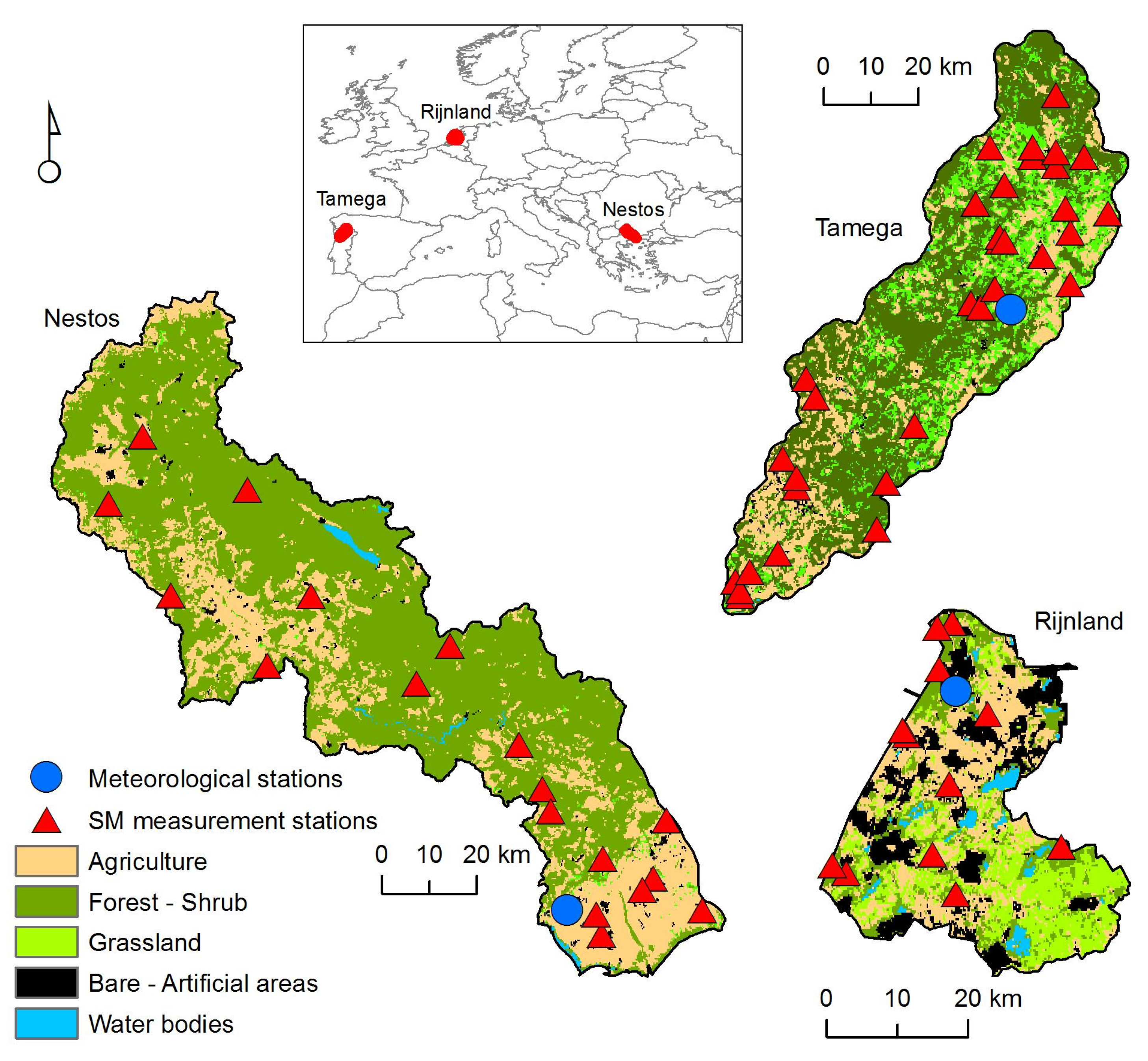
2.1.1. The Nestos River
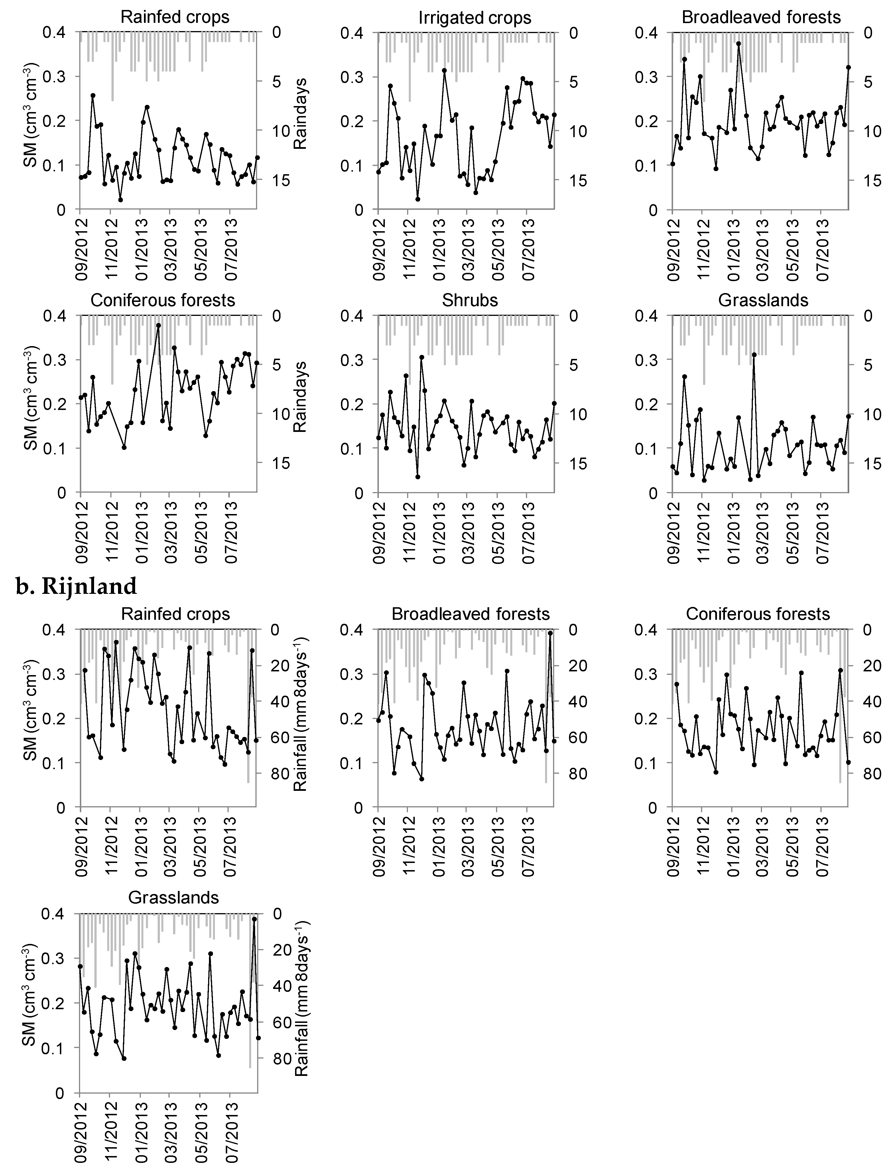
The Nestos is a transboundary river between Greece and Bulgaria. Its watershed covers an area of 6100 km2. Water is used for energy production and irrigation. The land cover is mainly natural vegetation (60%), and the rest is agricultural land. The climate is Mediterranean-continental, with a mean annual precipitation of 750 mm. Soil texture is mostly medium and fine along the river valley.

2.1.2. Rijnland

Rijnland is a low-lying area of land surrounded by dikes with an artificially-controlled water system using canals, pumps and weirs (polder) in the western part of the Netherlands, bordering the North Sea. The total area is about 1000 km2, of which the majority (72%) is occupied by low-lying land reclamation areas, while 15% is covered by free-draining areas and 8% by dunes. The area consists of urban and rural sectors committed to horticulture, agriculture and grasslands. The climate is temperate-maritime, and the annual precipitation is 960 mm. Soil texture is coarse on the northwest side along the coast, medium in the central area and medium-fine in the southern section of the study area.

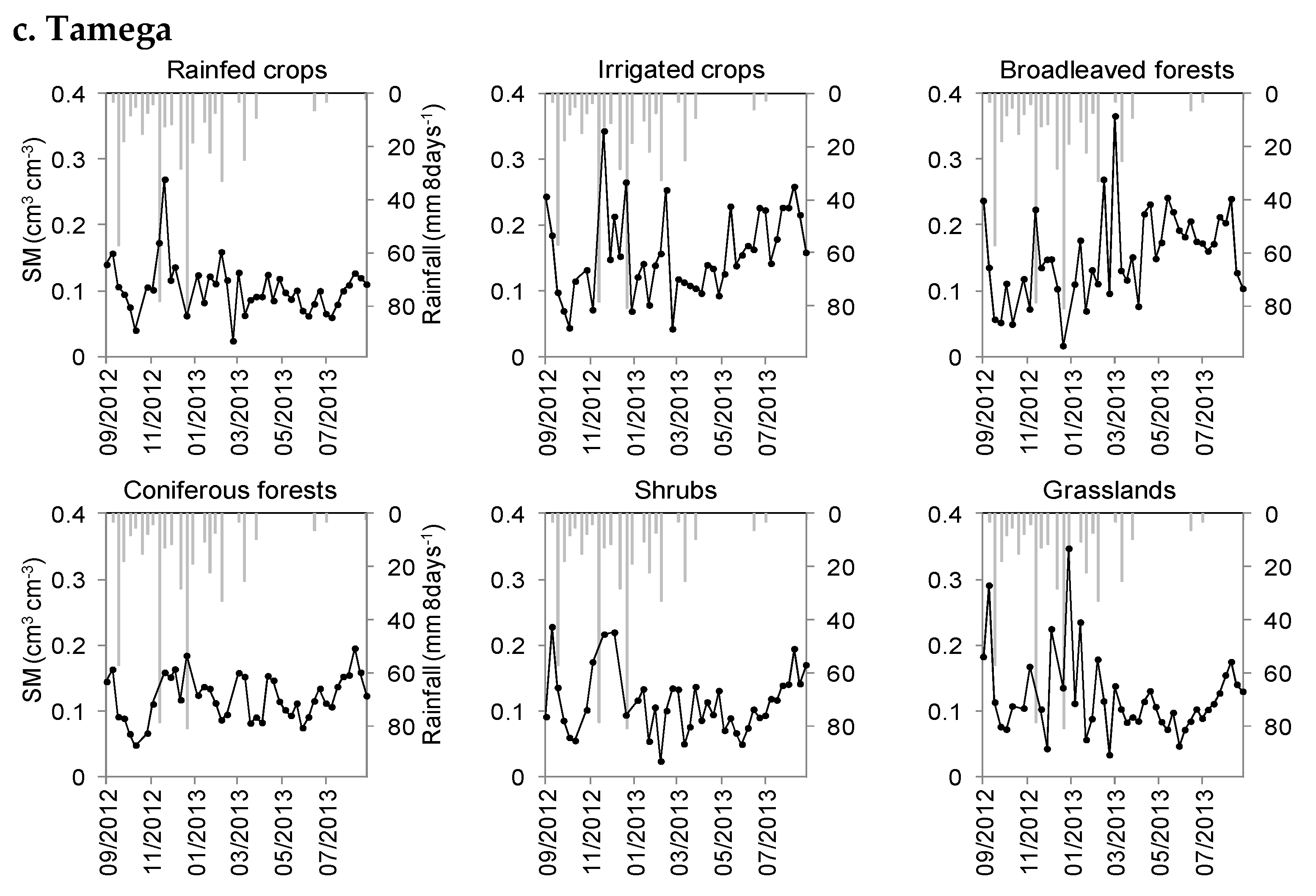
2.1.3. The Tamega River

The Tamega is a transboundary river between Portugal and Spain and is a tributary of River Douro. Its watershed has an area of approximately 3270 km2 and drains to the Torrao reservoir. The main land cover types are forest (65%) and agriculture (31%). The climate is warm temperate-Mediterranean, and the mean annual precipitation is 850 mm. Soil texture is medium throughout the study area.

2.2. Data and Pre-Processing

Several products from the MODIS (Moderate Resolution Imaging Spectroradiometer) instrument aboard the Terra (formerly known as Earth Observing System—EOS AM) satellite were used:
  • MODIS surface reflectance (MOD09Q1, MOD09A1) provides an estimate of the surface spectral reflectance at a 250- and a 500-m spatial resolution, as would have been measured at ground level in the absence of atmospheric scattering or absorption.
  • MODIS global land surface temperature (LST) and emissivity (MOD11A2) are estimated using the split-window technique on the thermal bands of MODIS at a 1-km spatial resolution.
The above-mentioned products are 8-day composites, meaning that each pixel contains the best possible observation during an 8-day period as selected on the basis of high observation coverage, low view angle, the absence of clouds or cloud shadow and aerosol loading. Additional data provided with these products include quality assessment, the day of the year for the pixel, along with solar, view and zenith angles. The quality assessment information of each MODIS Land HDF-EOS (Hierarchical Data Format-EOS) data product was utilized in order to remove low quality pixels using the LDOPE software tools provided by the MODIS Land Quality Assessment [19]. The products mentioned above are validated Stage 2, meaning that accuracy has been assessed over a widely-distributed set of locations and time periods via several ground truth and validation efforts [20]. For instance, the accuracy of MODIS LST is better than 1 °C, when validated with daily in situ data [21,22] and better than 2 °C using nighttime ground measurements [23].
Saturated water content (θs) was used as an input dataset for the estimation of SM. θs was estimated by Joint Research Centre (JRC)/Soil Bureau using pedotransfer functions as described in Tóth et al. [24]. The prediction method was used depending on the type of available input information, which were the Database of Hydraulic Properties of European Soils (HYPRES) [25], the Hungarian Detailed Soil Hydrophysical Database (MARTHA) [26] and the Soil Map of the Region of Eastern Macedonia and Thrace [27] datasets. The accuracy of estimations reached an RMSE (vol%) of 3.437 and a Pearson correlation coefficient of 0.857 (p = 0.01) with the measured data.
An updated map of land cover was created per study area. Multispectral SPOT XS and Landsat 5 TM satellite images were used, together with Web Map Service data (Google Earth) and in situ observations, in an automated supervised classification to produce the map of the main land cover types [28].
Raster meteorological data were utilized instead of point measurements from ground meteorological stations, in order to account for the large spatial variability within each catchment and the sparse coverage of ground station observations. The raster meteorological data were provided by the Center for Weather Forecast and Climate Analysis/Brazilian National Institute for Space Research (CPTEC/INPE). The CPTEC/INPE configured its regional Eta model to run for the study areas with a 5-km horizontal resolution and boundary conditions from CPTEC/INPE Global Model, T213L42 version. The initial conditions were obtained from the GFS (Global Forecast System) numerical model of the NCEP/NOAA (National Centers for Environmental Prediction/National Oceanic and Atmospheric Administration). The ETA model was executed daily at 00 and 12 Zulu time (GMT) and provided forecasts with a one-hour time step up to 3 days ahead. The 24-hour forecasts were used to avoid the transient errors from the initial stabilization of the model results before getting optimum accuracy. Table 1 lists the meteorological parameters that were used in further analyses.
Rainfall data were gathered from at least one rain gauge lying within each study area. Precipitation heights were recorded daily, with the exception of the Chrysoupoli meteorological station in Nestos that recorded the presence of precipitation events daily. Thus, the information from this station was used qualitatively.
Table 1. List of meteorological parameters that were used.
Parameter NameUnit
Surface downward short wave flux(W/m2)
2 m relative humidity(%)
2 m temperature(K)
10 m u wind (zonal component)(m/s)
10 m v wind (meridional component)(m/s)
Field surveys were conducted before and during the study period to collect in situ measurements of soil moisture in order to assess the accuracy of the results. A stratified random sampling was adopted for reducing the number of samples, while at the same time maintaining the desired level of accuracy. The strata were defined from overlay analysis of broad vegetation and soil texture categories from recent satellite images and soil parameter maps. The number of sample sites per stratum was determined as a function of SM variability and the desired accuracy in the estimations [29]. Their location was determined randomly using a GIS function. In each sample location, soil moisture measurements were conducted on at least 15 sub-locations, spread around the sample location, aiming to cover the variability within the satellite pixel [30]. The soil moisture was measured with a FieldScout TDR probe. The instrument is based on time domain reflectometry, where the apparent dielectric constant of the soil matrix (Ka) is determined using an electrical field and is empirically related to the volumetric soil moisture content. The TDR was previously calibrated using 50 soil core samples covering a wide range of soil types and moisture contents, where soil moisture was measured with the gravimetric method (R2 = 0.857, p < 0.01). Soil moisture was recorded using the 7.5–20-cm probes, and basic soil observations were noted.

2.3. Methods for Estimating Soil Moisture with Thermal Infrared Satellite Images

Soil moisture in the root zone (θrz) was estimated using the following equation [13]:
θ r z = θ s a t  exp ( Λ 1 0.42 )
where θsat is the saturated water content and Λ is the evaporative fraction. θsat is a normalization term, so that when the relative soil moisture ( θ r z θ s a t ) reaches 1 (soils fully saturated), the soil moisture θrz equals the soil porosity.
The evaporative fraction (Λ) is the ratio between the latent heat flux (λE) that is the energy consumed for evapotranspiration and the net available energy that is the net radiation (Rn) minus soil heat flux (G0).
Λ = λ E R n G 0
Under non-advective conditions, the Λ values ranges usually between 0 and 1, which represents zero to maximum evapotranspiration [31].
Τhe latent heat flux (λE) is derived using the energy balance equation:
λ E = R n G 0 H
The net radiation represents the actual energy available at the surface resulting from the total incoming short and longwave radiation and its loss through various processes (evapotranspiration, heat production, metabolic activities) [32].
R n =   ( 1 a )   K i n + L i n L o u t ( 1 ε 0 )   L i n
where α is the albedo, ε0 is the emissivity, Kin is the shortwave input radiation and Lin is the incoming longwave radiation defined as:
L i n = ( 1.08   ( ln τ s w ) 0.265 )   5.67   10 8   T a 4
Lout corresponds to the outgoing longwave radiation and is calculated as a function of the surface temperature (Ts) and ε0:
L o u t = ( ε 0   5.67   10 8   T s 4 )
The soil heat flux G0 refers to the heat stored in the soil and the vegetation. Having estimated Rn, G0 can be easily deduced through the following expression:
G 0 = R n ( T s 273 )   ( 0.0032 a 0.9 + 0.0062 ( a 0.9 ) 2 )   1 0.978   N D V I 4 a
In the above equations, Ts, ε0, α and the Normalized Difference Vegetation Index (NDVI) are intermediate variables computed using the MODIS data using conventional equations. The shortwave transmissivity (τsw), Ta and Kin are derived from meteorological data output from the weather forecast model.
The sensitive heat flux (H) corresponds to the heat loss to the air due to the temperature difference, as shown by the equation below:
H = C p   ρ   d T r a h
where Cp is the air specific heat, ρ is the air density, rah is the aerodynamic resistance to heat transport and dT is the difference between soil and air temperatures. The accurate computation of H using raster meteorological data is detailed in [33].
The latent heat flux, thus the evaporative fraction, is relative to the whole root zone, so root depth and soil depth maps were used to estimate the θsat information, using a linear relation.
In order to solve the energy balance equation, a variation of the SEBAL algorithm was used. Alexandridis et al. [34] developed the “ITA-Water” tool (Integrated Thermodynamic Algorithms for Estimating Agricultural Water Use) for the implementation of the SEBAL approach using Terra MODIS composite images. Based on this tool and considering the requirements for using spatially-distributed meteorological data, the tool evolved into the “ITA-MyWater”, and its functionalities were extended to estimate the soil moisture at the root zone [33].

3. Results and Discussion

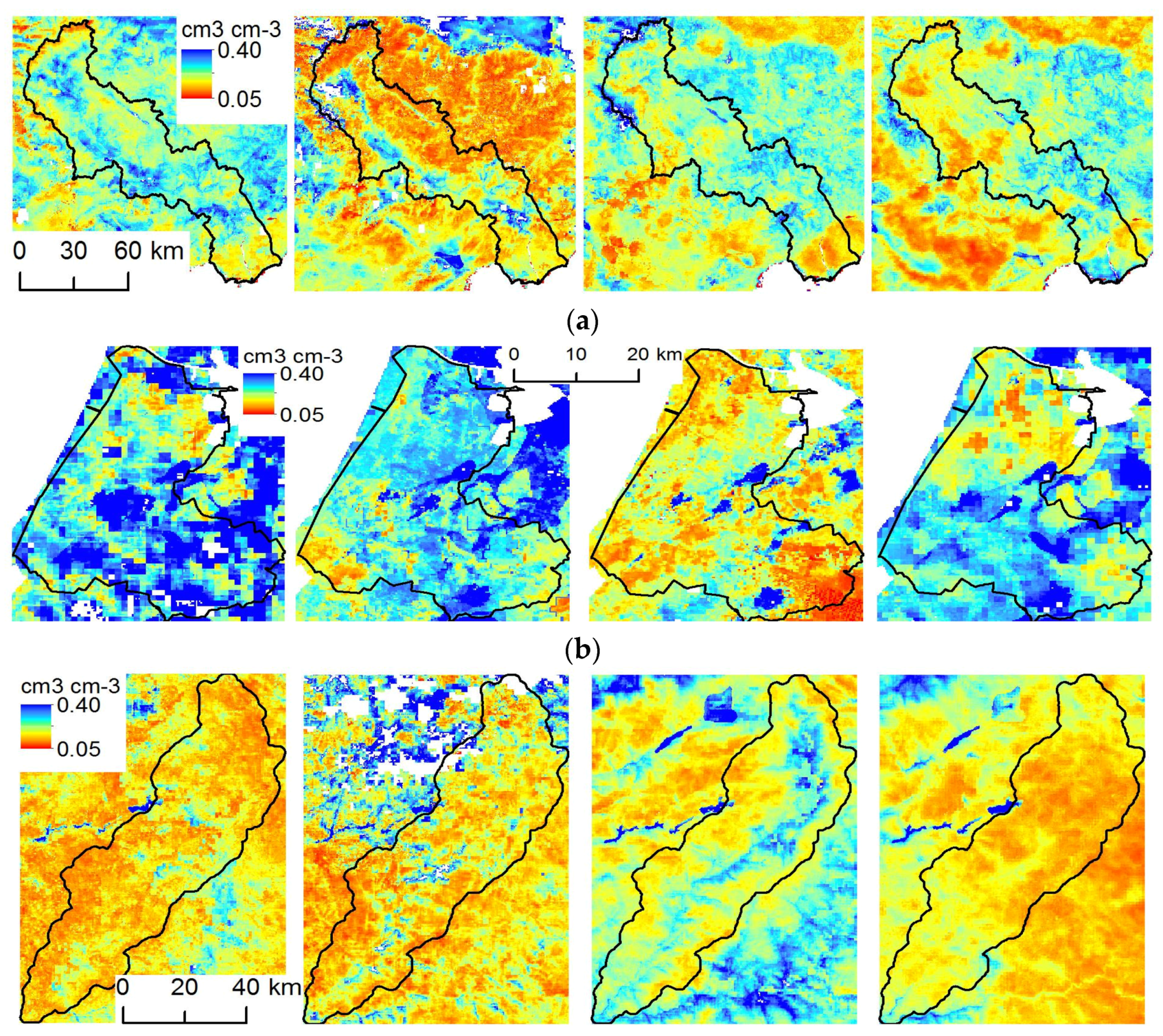
3.1. Spatial Patterns of Soil Moisture

Four SM maps per site were selected from the time series to show the spatial variability of each study area at various seasons (Figure 2). One-way analysis of variance (ANOVA) on a per-pixel basis was used to examine the effects of land cover and soil texture on the selected SM maps for each basin and to interpret its spatial patterns [35,36]. The results are presented as SM mean and standard deviation for each class, as well as the level of significance of the differences between classes (Table 2 and Table 3).
Table 2. SM means and standard deviations per land cover type (cm3·cm−3).
Land coverNestosRijnlandTamega
Rainfed crops0.11/0.05 a0.22/0.09 a0.10/0.04 a
Irrigated crops0.16/0.08 bn/a0.16/0.07 b
Broadleaved forests0.20/0.06 c0.18/0.07 b0.15/0.07 b
Coniferous forests0.22/0.07 c0.18/0.06 b0.12/0.03 c
Shrubs0.15/0.05 bn/a0.11/0.05 a
Pastures0.11/0.06 a0.20/0.07 a0.12/0.06 c
Note: Different letters give significant differences within each column (p < 0.001).
Table 3. SM means and standard deviations per soil texture class (cm3·cm−3).
Soil Texture NestosRijnlandTamega
Fine0.19/0.06 a0.23/0.11 an/a
Medium 0.18/0.07 b0.22/0.09 b0.13/0.06
Coarse0.16/0.06 c0.18/0.07 cn/a
Note: Different letters give significant differences within each column (p < 0.001).
Figure 2. Spatial variability of SM in the study areas: (a) Nestos 24 November 2012, 1 January 2013, 9 May 2013, 18 June 2013; (b) Rijnland 7 October 2012, 25 January 2013, 18 February 2013, 5 August 2013; (c) Tamega 7 October 2012, 24 November 2012, 1 January 2013, 4 August 2013. No-data pixels appear in white.
Water 08 00032 g002
The spatial variability of SM in the Nestos basin (Figure 2a) follows the meteorological conditions, as well as the main geomorphological features. Lower values of SM were observed in the areas covered by rainfed crops, shrubs and pastures (Table 2). Significantly higher values were estimated in the forested areas, which appear towards the elevated middle parts of the study area. For the selected dates of Figure 2a, SM was high in most parts on 25 November 2012 following a few rain events and higher on 9 May 2013 after four consecutive rainy days. SM was lower than 0.15 cm3 cm−3 in most parts of the study site, with the exception of the river’s narrow valley, which is characterized by higher values of SM even during dry periods, being at the lowest end of the natural drainage system and dominated by medium to fine clays (Table 3). SM values were low in the northern part of the study site on 18 June 2013, but very high in the eastern and southern ends. This map captures the peak of the irrigation season and shows high values of SM at the irrigation network that has been developed in the river’s floodplain at the southern end of the study area.
The spatial variability of SM in Rijnland is guided by the meteorological conditions, as well as the main soil types and shallow water table regime, closely connected to a dense surface water network of lakes and canals (Figure 1). SM is higher throughout the catchment, as compared to the other study areas. The natural vegetation of the north and western end of the study area have significantly lower SM than the pastures at the southeast (Table 2). The areas surrounding the water bodies at the central and western side display the highest SM on all occasions, being dominated by medium to fine texture soils (Table 3). SM on 7 October 2012 (Figure 2b) was high in the study area (0.20–0.35 cm3·cm−3) following a few days of rainfall. Similarly high SM appeared on 25 January 2013 in the central and northern parts of the study area (0.18–0.30 cm3·cm−3), following a smaller rain event. SM values were much lower (0.15–0.25 cm3·cm−3) on 28 February 2013, which followed several dry days. On 5 August 2013, SM was low in the north (0.09–0.22 cm3·cm−3) and higher at the southern half of the study area (0.26–0.38 cm3·cm−3), following a local rain event, as reported by the meteorological station.
The spatial variability of SM in the Tamega basin follows the meteorological conditions, as well as the main geomorphological features and the high land cover variability (Figure 1). Lower values appear at the mountain tops, where sparse vegetation, barren land and rocks dominate, and significantly higher values at the narrow river valley towards the centerline of the study area (Table 2). The soil texture is uniform, thus appearing to have no impact on the spatial pattern of SM (Table 3). SMs on 7 October 2012 and 1 January 2013 (Figure 2c) were low overall (0.08–0.18 cm3·cm−3 and 0.13–0.2 cm3·cm−3, respectively), following a dry period, with the exception of the land along the river, where SM was very high (0.23–0.30 cm3·cm−3 and 0.31–0.38 cm3·cm−3, respectively). On 24 November 2012, SM was very high in the northwest end of the study area, where a recent rainfall had occurred (evident around the cloud-covered pixels), while it was lower at the southern parts. On 4 July 2013, SM was very low throughout the study area (0.08–0.15 cm3·cm−3), with the exception of the agricultural land on the southern end, where SM was kept close to 0.20 cm3·cm−3 via irrigation.

3.2. Temporal Dynamics of Soil Moisture

Figure 3 shows the time series of SM at selected locations, one per land cover type (Figure 1). SM of rainfed crops in Nestos (Figure 3a) was governed by the temporal distribution of rain events: it showed an undulating pattern with higher values (>0.2 cm3·cm−3) during the rainy seasons of autumn (October–November) and spring (February–March). During the dry summer season, SM fell to lower values (0.07–0.17 cm3·cm−3), which is, nevertheless, after the harvest of the winter cereals. SM of irrigated crops was similar to the SM of rainfed crops during the wet months (October–May) and then remained high (0.15–0.3 cm3·cm−3) during the irrigation season (June–September). SM of broadleaved forests was high during the wet winter season (0.17–0.35 cm3·cm−3) and dropped to lower values (0.13–0.25 cm3·cm−3) during the dry summer months. The high values during the wet season were due to the north-facing slopes and the higher altitude at which the broadleaved forests appear, where evaporation was lower. SM of coniferous forests was stable throughout the year (0.1–0.3 cm3·cm−3), with slightly higher values during the wet spring and late summer, probably due to the frequent storms at the high altitudes in which this vegetation type appears. SM of shrubs and pastures fluctuated in accordance with the temporal distribution of rain events, mostly during the wet season, similar to rainfed crops. SM of pastures was lower than the others with the highest temporal fluctuation, possibly because they are located in shallow soils.
SM in Rijnland was higher, compared to the other study areas, with higher minima (Figure 3b). SM temporal patterns of broadleaved forest, coniferous forest and pastures were similar with a higher temporal variation (standard deviations ranging from 0.06 to 0.09 cm3·cm−3). SM of rainfed crops was the highest of all examined land cover types (annual average 0.22 cm3·cm−3). SM of all land cover types related directly to the pattern of rainfall during most of the year, with the exception of summer, when the phreatic water level was artificially risen (by either letting in additional water or applying less drainage) and fed the soil moisture, even at times of lower rainfall. Similar temporal patterns had been experienced in a location to the east of Rijnland; however, the recorded SM had reached higher values in the first quarter of 2002 [37]. The exceptionally high soil moisture of mid-September 2013 was due to the heavy rainfall of these days, which had influenced the SM of all examined land cover types.
In Tamega (Figure 3c), there was higher SM and variability (0.05–0.35 cm3·cm−3) during the winter–spring wet period (December–March), which dropped during the dryer summer months (0.08–0.15 cm3·cm−3). SM rose again in September after the small, but frequent rain events. SM of rainfed crops, coniferous forests, shrubs and pastures followed the pattern of rainfall, with peaks during the wet season. Irrigated crops followed a similar pattern during the winter; however, they displayed constantly higher values (0.14–0.26 cm3·cm−3) during the summer irrigation season (June–September). Broadleaved forests also displayed exceptionally high values during the summer months, due to the high altitude and sporadic storms. Despite the frequent precipitation events during November, all land cover types had low SM, due to its low intensity. Similar temporal patterns had been noted for the forested area adjacent to the east catchment for the previous hydrological year, when some extreme SM values had been noted during winter 2011 [8].
Figure 3. Time-series of SM at the selected locations per land cover and rainfall in the study areas: (a) Nestos; (b) Rijnland; and (c) Tamega.
Water 08 00032 g003aWater 08 00032 g003b

3.3. Validation and Analysis of Environmental Parameters

Comparison of the remotely-sensed estimations of SM was performed with in situ measurements of SM for the top-soil acquired during the field surveys. The correlation coefficient, the Student’s t-test and the RMSE were calculated. The results are presented in Table 4.
For Nestos, the relationship between remotely-sensed SM estimates and in situ measurements was high and statistically significant during the summer period and low during the winter season (r = 0.62 and 0.36, respectively). It was not possible to establish any relation during the field survey of April 2013, as the satellite images were influenced by consistently cloudy weather. The RMSE was low throughout the seasons, ranging from 0.037 to 0.055 cm3·cm−3. The mean differences were mostly positive, revealing an underestimation of remotely-sensed SM as compared to in situ measurements.
Table 4. Correlation coefficients, RMSE and mean differences of field-surveyed vs. remote sensing data.
Study AreaDate of Field SurveyCountrRMSE (cm3·cm−3)Mean difference (cm3·cm−3)
Nestos13–15 July 2011200.62 *0.0370.004
Nestos3–5 November 2012220.360.0410.057 **
Nestos9–10 April 201327-0.0550.043 *
Nestos2–3 July 2013240.42 *0.039−0.042 **
Rijnland17–19 July 2012170.370.0760.061 **
Rijnland26–29 June 2013250.310.0870.091 **
Rijnland23–26 September 2013220.52 *0.0860.039
Tamega26–29 September 2011280.43 *0.015−0.062 **
Tamega20–23 May 2013380.310.0230.044 **
Tamega2–5 September 201338-0.024−0.070 **
Note: * Statistically significant at the 0.05 level; ** statistically significant at the 0.001 level.
In Rijnland, the relationship between SM estimates and measurements was high in June and July (r = 0.31 and 0.37, respectively) and even higher and statistically significant in September (r = 0.52). The RMSE and mean differences were amongst the highest across the study sites (<0.087 cm3·cm−3 and <0.091 cm3·cm−3, respectively). The mean differences were consistently positive, revealing an underestimation of remotely-sensed SM as compared to in situ measurements.
In Tamega, the relationship between SM estimates and measurements was high and statistically significant in September 2011 and medium in May 2013, but it was not possible to establish any relation during September 2013, when soil moisture was too low, almost reaching the low measurable range of the TDR. The RMSE was low (<0.024 cm3·cm−3), and the mean differences were medium to low, but of a variable sign. Similar accuracy was reported for the catchment adjacent to Tamega and the previous hydrological year, where errors were lower during the spring and summer seasons [8].
The relationships between SM estimates and in situ measurements were variable. This can be explained by several factors, such as the temporal difference between the datasets, rain events during the measurements and the scale difference. The effect of these factors was evaluated using one-way analysis of variance (ANOVA) of the residuals between measured and estimated SM, for a selected field survey, per study area. The results are presented as p-values and the level of significance of the parameter’s effect, where low p-values denote a high confidence that there is an actual difference caused by the parameter (Table 5).
MODIS data were acquired daily for each location and then put together in eight-day composites, which means that each pixel of the SM map may refer to a different day within the respective eight-day period. Therefore, the estimated SM may be as much as eight days apart from the measured SM. At the same time, soil moisture has been reported to vary greatly, even daily, depending on topography, soil properties and meteorological conditions [38].
The temporal difference between the measured and estimated SM ranged from −2 to 3 days in Nestos, from 3 to 5 in Rijnland and from −3 to 1 days in Tamega (negative temporal difference means that the estimation preceded the measurement). This effect has significant influence at the Rijnland and Tamega sites (p = 0.003 and 0.026, respectively), but not at Nestos (p = 0.389), possibly because the meteorological conditions have increased the influence of temporal variation of SM in the first two sites.
Field surveys required from 2 to 4 days to cover each case study catchment. During this time, there was a possibility of rain on the whole or part of the site. This was expected to influence the quality of the measurements, especially if the rain event were between the times of in situ measurement and satellite overpass.
During the selected field surveys, there was a single rain event in Tamega and multiple ones in Rijnland, while there was dry weather in Nestos. The rain events seem to significantly influence the quality of the results in Rijnland (p = 0.023), but not in Tamega (p = 0.114), probably because the rain event in Tamega was very light.
The field surveys provided point measurements, spread around the sampling location to describe at an adequate level the local variability of SM. However, the comparison with the large MODIS pixels (250 m) was expected to show a deviation, especially at the most heterogeneous locations. The level of heterogeneity of land cover at each location was evaluated with the landscape metric Shannon’s Diversity Index (SHDI) [39]. The SHDI of each location was compared to the residuals to identify the level of influence of the scale difference between the point measurements and the MODIS observations, providing no significant influence on the quality of the results (p > 0.501 at all sites). This verified that the measurement locations were correctly selected in large homogeneous areas.
Table 5. Analysis of variance and the effect of various parameters on the residuals at all sites (p-values).
Study AreaDate of Field SurveyTemporal DifferenceRain EventLocation Heterogeneity
Nestos13–15 July 20110.389-0.618
Rijnland17–19 July 20120.003 *0.023 *0.712
Tamega26–29 September 20110.026 *0.1140.501
Note: * Statistically significant at the 0.05 level.

4. Discussion

The temporal variability of SM is routinely measured by automated soil moisture probes, which is useful for a field or other homogeneous area. A time series of spatially-distributed measurements for the entire catchment is, however, not feasible. The importance of this work consists in providing continuous time series of SM maps at the catchment scale. The main advantages of the methodology are that it avoids some basic problems reported in SM mapping with remote sensing, such as the bias of dense vegetation and surface roughness of microwave images, and the influence of surface reflectance variability of the visible and near-infrared images [40,41].
Input MODIS products surface reflectance and LST were eight-day composites, which offer the advantage of improved data quality at the pixel level. However, some cloud effects cannot be successfully removed, such as the cloud shadow [42] and artificial heterogeneity [43]. Persistent cloud cover for more than eight days could be dealt with by using longer compositing periods (e.g., 16 days or one month); however, there is a risk of losing important phenological changes of crops with short growing seasons [44,45].
The partitioning of surface fluxes, in this case Λ, was used as an indicator of SM based on the argument that the observed difference between the actual and potential evapotranspiration is caused by the available water in the root zone [13]. The importance of SM on the evapotranspiration process of plants has been reported positively in dry and negatively in wet climates [37]. Nevertheless, similar methods have provided successful results in various climates (Pakistan, Mexico, Brazil, Ghana and others), at extreme conditions (near the permanent wilting point of crops or at field capacity), using Landsat and MODIS satellite images [13,46,47].
Deviations of remote sensing estimates from in situ measurements were comparable to those obtained in the Iberian peninsula by the disaggregation of SMOS data to 500 m [8] and with those reported for the SMOS products [48]. A similar range of accuracy was reported by using surface energy fluxes in Pakistan and Mexico [13]. The almost consistent underestimation of SM by the satellite estimations as compared to in situ measurements was also noted by Sánchez–Ruiz, Piles, Sánchez, Martínez–Fernández, Vall–llossera and Camps [8], while Fang and Lakshmi [9] produced mixed results.
The observed higher temporal variability during the rainy season could be due to errors introduced by the frequent cloud cover and variable atmospheric conditions, the low performance of the MODIS compositing algorithm, as well as the uncertainty of the meteorological model used for input. Thus, there are occasions when the compositing algorithm underperforms and errors are introduced in the remote sensing estimations [49]. Nevertheless, using composited data is a routine method to overcome frequent cloud coverage and to minimize the gaps in time series, and techniques have been proposed to estimate the introduced error [50]. Akuraju et al. [51] point out some limitations in the use of an exponential model to fit soil moisture in the root zone to Λ. Indeed, the relation is sensitive to vegetation biomass, with a correlation significantly higher when there is enough biomass. In addition, Λ values depend on the ET limiting conditions (water or energy conditions); thus, Akuraju et al. (2013) advise to adapt the model to the NDVI and net radiation values, whether they are above or below certain thresholds. A time lag between rainfall events and SM increase can be noted in some cases, similar to related literature [8,41]. This could be due to the compositing within eight days of the satellite observations and the meteorological data. The in situ measurements were performed with a TDR that measures topsoil moisture (0–7.5 and 0–20 cm) and were compared to the estimated root zone SM in the study areas, which can vary from 0–0.3 m for grassland to 0–2 m for trees. Although they can vary differently in time, due to their non-linear relation, these two parameters can be compared, since each test site is located within a certain geoclimatic environment [16], under homogeneous bioclimatic conditions [52]. The comparison is more efficient in wet conditions [35]. Ford et al. [53] demonstrated that there is generally a strong relationship between near-surface (5–10 cm) and root zone (25–60 cm) soil moisture in a study conducted in an extensive area (Great Planes, USA), while Ragab [18] used an empirical relationship to estimate root-zone soil moisture from surface soil moisture. Using a limited number of in situ observations to validate a remote sensing product is acceptable, considering the associated cost of wide-scale field surveys and the spatial representativeness of the sampling design [54,55].
The presented methodology is a semi-automated procedure. Several tools have been prepared to facilitate the operation by the analyst [33,34,56]. It uses freely available data at no cost from operational satellites, meteorological models and soil data. Alternative sources of satellite data can be used, such as Aqua MODIS, NOAA AVHRR or other satellites with visible, near and thermal infrared bands.
The presented eight-day SM maps are essential for water and land management studies. They are useful as inputs in meteorological, hydrological, gas and energy exchange models. Yet, SM is very dynamic and influenced by multiple factors, thus difficult to model [57]. They can be directly inserted into models or they can provide a means for calibration and operational adjustment (through data assimilation) of the spatial distribution of hydrological parameters [2,3,4,18].

5. Summary and Conclusions

An integrated methodology was presented that connects the evaporative fraction, as an indicator of SM, with MODIS satellite images, which offer frequent, global, validated and free of cost data and, therefore, allow for operational monitoring applications.
The methodology was tested in three diverse European environments. The resulting maps were successfully validated using in situ measurements, slightly underestimating SM, but the RMSE was comparable to similar attempts found in the literature.
Several factors were analyzed to explain the variation in the accuracy, and it was shown that the land cover type, the soil texture class, the temporal difference between the datasets acquisition and the presence of rain events during the measurements played a significant role, unlike the scale difference between in situ and satellite observations.
Therefore, the proposed methodology can be used operationally to estimate SM maps at the catchment scale, with a 250-m spatial resolution and eight-day time step.

Acknowledgments

The work presented is part of the FP7-EU project MyWater “Merging hydrological models and Earth observation data for reliable information on water”. Terra MODIS satellite images were provided by USGS.

Author Contributions

T.K. Alexandridis and I. Cherif designed the methodology, performed the experiments and wrote the paper. G. Bilas, W.G. Almeida, I.M. Hartanto, S.J. van Andel and A. Araujo contributed to the conception and design of the experiments, as well as to the data analysis.

Conflicts of Interest

The authors declare no conflict of interest.

References

  1. Wagner, W.; Bloschl, G.; Pampaloni, P.; Calvet, J.C.; Bizzarri, B.; Wigneron, J.P.; Kerr, Y. Operational readiness of microwave remote sensing of soil moisture for hydrologic applications. Nord. Hydrol. 2007, 38, 1–20. [Google Scholar] [CrossRef]
  2. Ottlé, C.; Vidal-Madjar, D. Assimilation of soil moisture inferred from infrared remote sensing in a hydrological model over the hapex-mobilhy region. J. Hydrol. 1994, 158, 241–264. [Google Scholar] [CrossRef]
  3. Song, Y.; Hartanto, I.M.; Alexandridis, T.; van Andel, S.J.; Solomatine, D.P. Frequency analysis of earth observation and hydrological model evapotranspiration and soil moisture. In Geophysical Research Abstracts; EGU2014-15887; European Geosciences Union General Assembly: Vienna, Austria, 2014. [Google Scholar]
  4. Hartanto, I.M. Merging earth observation data, weather predictions, in-situ measurements, and hydrological models, for water information services. Environ. Eng. Manag. J. 2015, 14, 2031–2042. [Google Scholar]
  5. NOAA-SSM/I. National Oceanic and Atmospheric Administration (NOAA) Special Sensor Microwave/Imager (Ssm/I) Product. Available online: http://www.osdpd.noaa.gov/ml/spp/sharedprocessing.html#SM (accessed on 13 March 2015).
  6. SMOS-ESA. Soil Moisture Ocean Salinity (SMOS) Mission. Available online: https://earth.esa.int/web/guest/missions/esa-operational-eo-missions/smos (accessed on 13 March 2015).
  7. Bartalis, Z.; Wagner, W.; Naeimi, V.; Hasenauer, S.; Scipal, K.; Bonekamp, H.; Figa, J.; Anderson, C. Initial soil moisture retrievals from the metop—A advanced scatterometer (ASCAT). Geophys. Res. Lett. 2007, 34. [Google Scholar] [CrossRef]
  8. Sánchez-Ruiz, S.; Piles, M.; Sánchez, N.; Martínez-Fernández, J.; Vall-llossera, M.; Camps, A. Combining smos with visible and near/shortwave/thermal infrared satellite data for high resolution soil moisture estimates. J. Hydrol. 2014, 516, 273–283. [Google Scholar] [CrossRef]
  9. Fang, B.; Lakshmi, V. Soil moisture at watershed scale: Remote sensing techniques. J. Hydrol. 2014, 516, 258–272. [Google Scholar] [CrossRef]
  10. Oh, Y.; Sarabandi, K.; Ulaby, F.T. An empirical model and an inversion technique for radar scattering from bare soil surfaces. IEEE Trans. Geosci. Remote Sens. 1992, 30, 370–381. [Google Scholar] [CrossRef]
  11. Fung, A.K.; Li, Z.; Chen, K.S. Backscattering from a randomly rough dielectric surface. IEEE Trans. Geosci. Remote Sens. 1992, 30, 356–369. [Google Scholar] [CrossRef]
  12. Baghdadi, N.; Abou Chaaya, J.; Zribi, M. Semiempirical calibration of the integral equation model for sar data in c-band and cross polarization using radar images and field measurements. IEEE Geosci. Remote Sens. Lett. 2011, 8, 14–18. [Google Scholar] [CrossRef]
  13. Scott, C.A.; Bastiaanssen, W.G.M.; Ahmad, M.U.D. Mapping root zone soil moisture using remotely sensed optical imagery. J. Irrig. Drain. Eng. 2003, 129, 326–335. [Google Scholar] [CrossRef]
  14. Bastiaanssen, W.G.M.; Molden, D.J.; Makin, I.W. Remote sensing for irrigated agriculture: Examples from research and possible applications. Agric. Water Manag. 2000, 46, 137–155. [Google Scholar] [CrossRef]
  15. Ahmad, M.U.D.; Bastiaanssen, W.G.M. Retrieving soil moisture storage in the unsaturated zone using satellite imagery and bi-annual phreatic surface fluctuations. Irrig. Drain. Syst. 2003, 17, 141–161. [Google Scholar] [CrossRef]
  16. Sabater, J.M.; Jarlan, L.; Calvet, J.-C.; Bouyssel, F.; de Rosnay, P. From near-surface to root-zone soil moisture using different assimilation techniques. J. Hydrometeorol. 2007, 8, 194–206. [Google Scholar] [CrossRef]
  17. Manfreda, S.; McCabe, M.F.; Fiorentino, M.; Rodríguez-Iturbe, I.; Wood, E. Scaling characteristics of spatial patterns of soil moisture from distributed modelling. Adv. Water Resour. 2007, 30, 2145–2150. [Google Scholar] [CrossRef]
  18. Ragab, R. Towards a continuous operational system to estimate the root-zone soil moisture from intermittent remotely sensed surface moisture. J. Hydrol. 1995, 173, 1–25. [Google Scholar] [CrossRef]
  19. Roy, D.P.; Borak, J.S.; Devadiga, S.; Wolfe, R.E.; Zheng, M.; Descloitres, J. The modis land product quality assessment approach. Remote Sens. Environ. 2002, 83, 62–76. [Google Scholar] [CrossRef]
  20. NASA—Land Processes Distributed Active Archive Center. Land Surface Temperature & Emissivity 8-Day l3 Global 1 km (Mod11a2). Available online: https://lpdaac.usgs.gov/products/modis_products_table/mod11a2 (accessed on 20 July 2012).
  21. Wan, Z.; Zhang, Y.; Zhang, Q.; Li, Z.-L. Validation of the land-surface temperature products retrieved from terra moderate resolution imaging spectroradiometer data. Remote Sens. Environ. 2002, 83, 163–180. [Google Scholar] [CrossRef]
  22. Wan, Z.; Zhang, Y.; Zhang, Q.; Li, Z.-L. Quality assessment and validation of the modis global land surface temperature. Int. J. Remote Sens. 2004, 25, 261–274. [Google Scholar] [CrossRef]
  23. Wang, W.; Liang, S.; Meyers, T. Validating modis land surface temperature products using long-term nighttime ground measurements. Remote Sens. Environ. 2008, 112, 623–635. [Google Scholar] [CrossRef]
  24. Tóth, B.; Weynants, M.; Nemes, A.; Makó, A.; Bilas, G.; Tóth, G. New generation of hydraulic pedotransfer functions for europe. Eur. J. Soil Sci. 2015, 66, 226–238. [Google Scholar] [CrossRef] [PubMed]
  25. Wösten, J.; Lilly, A.; Nemes, A.; le Bas, C. Development and use of a database of hydraulic properties of european soils. Geoderma 1999, 90, 169–185. [Google Scholar] [CrossRef]
  26. Makó, A.; Tóth, B.; Hernádi, H.; Farkas, C.; Marth, P. Introduction of the hungarian detailed soil hydrophysical database (martha) and its use to test external pedotransfer functions. Agrokém. Talajt. 2010, 59, 29–38. [Google Scholar] [CrossRef]
  27. Misopolinos, N.; Silleos, N.; Bilas, G.; Karapetsas, N.; Barbagiannis, N.; Panagiotopoulos, K.; Haidoudi, K.; Zalidis, G. Assessment of Nutrients, Heavy Metals and hydrodynamic Soil Properties for the Wise Use of Water and Fertilizers and the Growth of Safe Products in the Region of Eastern Macedonia and Thrace; Final Report; Prefecture of East Macedonia and Thrace: Komotini, Greece, 2010. [Google Scholar]
  28. Nunes, Α.; Araujo, A.; Alexandridis, T.K.; Chambel, P. Effects of different scale land cover maps in watershed modelling. In Proceedings of the European Geosciences Union General Assembly, Vienna, Austria, 7–12 April 2013.
  29. Rao, R.G.S.; Ulaby, F.T. Optimal spatial sampling techniques for ground truth data in microwave remote sensing of soil moisture. Remote Sens. Environ. 1977, 6, 289–301. [Google Scholar] [CrossRef]
  30. Justice, C.O.; Townshend, J.R.G. Integrating ground truth data with remote sensing. In Terrain Analysis and Remote Sensing; Townshend, J.R.G., Ed.; Allen and Uniwin: London, UK, 1981; pp. 38–58. [Google Scholar]
  31. Bastiaanssen, W.G.M.; Menenti, M.; Feddes, R.A.; Holtslag, A.A.M. A remote sensing surface energy balance algorithm for land (SEBAL): 1. Formulation. J. Hydrol. 1998, 212–213, 198–212. [Google Scholar] [CrossRef]
  32. Allen, R.G.; Pereira, L.S.; Raes, D.; Smith, M. Crop Evapotranspiration: Guidelines for Computing Crop Water Requirements; FAO Irrigation and Drainage Paper; Food and Agriculture Organization of the United Nations: Rome, Italy, 1998. [Google Scholar]
  33. Cherif, I.; Alexandridis, T.K.; Jauch, E.; Chambel-Leitao, P.; Almeida, C. Improving remotely sensed actual evapotranspiration estimation with raster meteorological data. Int. J. Remote Sens. 2015, 36, 4606–4620. [Google Scholar] [CrossRef]
  34. Alexandridis, T.K.; Cherif, I.; Chemin, Y.; Silleos, G.N.; Stavrinos, E.; Zalidis, G.C. Integrated methodology for estimating water use in mediterranean agricultural areas. Remote Sens. 2009, 1, 445–465. [Google Scholar] [CrossRef]
  35. Heathman, G.C.; Larose, M.; Cosh, M.H.; Bindlish, R. Surface and profile soil moisture spatio-temporal analysis during an excessive rainfall period in the southern great plains, USA. Catena 2009, 78, 159–169. [Google Scholar] [CrossRef]
  36. Zhao, Y.; Peth, S.; Hallett, P.; Wang, X.; Giese, M.; Gao, Y.; Horn, R. Factors controlling the spatial patterns of soil moisture in a grazed semi-arid steppe investigated by multivariate geostatistics. Ecohydrology 2011, 4, 36–48. [Google Scholar] [CrossRef]
  37. Jacobs, A.F.; Heusinkveld, B.G.; Holtslag, A.A. Carbon dioxide and water vapour flux densities over a grassland area in the netherlands. Int. J. Climatol. 2003, 23, 1663–1675. [Google Scholar] [CrossRef]
  38. Hebrard, O.; Voltz, M.; Andrieux, P.; Moussa, R. Spatio-temporal distribution of soil surface moisture in a heterogeneously farmed mediterranean catchment. J. Hydrol. 2006, 329, 110–121. [Google Scholar] [CrossRef]
  39. Shannon, C.E. A mathematical theory of communication. Bell Syst. Tech. J. 1948, 27, 379–423. [Google Scholar] [CrossRef]
  40. Dobriyal, P.; Qureshi, A.; Badola, R.; Hussain, S.A. A review of the methods available for estimating soil moisture and its implications for water resource management. J. Hydrol. 2012, 458, 110–117. [Google Scholar] [CrossRef]
  41. Schnur, M.T.; Xie, H.; Wang, X. Estimating root zone soil moisture at distant sites using modis ndvi and evi in a semi-arid region of southwestern USA. Ecol. Inform. 2010, 5, 400–409. [Google Scholar] [CrossRef]
  42. Sousa, A.; Pereira, J.; Silva, J. Evaluating the performance of multitemporal image compositing algorithms for burned area analysis. Int. J. Remote Sens. 2003, 24, 1219–1236. [Google Scholar] [CrossRef]
  43. Langner, A.; Miettinen, J.; Siegert, F. Land cover change 2002–2005 in borneo and the role of fire derived from modis imagery. Glob. Chang. Biol. 2007, 13, 2329–2340. [Google Scholar] [CrossRef]
  44. Alexandridis, T.K.; Gitas, I.Z.; Silleos, N.G. An estimation of the optimum temporal resolution for monitoring vegetation condition on a nationwide scale using modis/terra data. Int. J. Remote Sens. 2008, 29, 3589–3607. [Google Scholar] [CrossRef]
  45. Chen, P.-Y.; Srinivasan, R.; Fedosejevs, G.; Kiniry, J. Evaluating different ndvi composite techniques using noaa-14 avhrr data. Int. J. Remote Sens. 2003, 24, 3403–3412. [Google Scholar] [CrossRef]
  46. Fleming, K.; Hendrickx, J.M.; Hong, S.-H. Regional mapping of root zone soil moisture using optical satellite imagery. Proc. SPIE 2005, 5811, 159–170. [Google Scholar]
  47. Hendrickx, J.M.; Honga, S.-H.; Friesenb, J.; Compaorec, H.; van de Giesenb, N.C.; Rodgersd, C.; Vlekd, P.L. Mapping energy balance fluxes and root zone soil moisture in the white volta basin using optical imagery. Proc. SPIE 2006, 6239. [Google Scholar] [CrossRef]
  48. Kerr, Y.H.; Waldteufel, P.; Wigneron, J.P.; Martinuzzi, J.; Font, J.; Berger, M. Soil moisture retrieval from space: The soil moisture and ocean salinity (SMOS) mission. IEEE Trans. Geosci. Remote Sens. 2001, 39, 1729–1735. [Google Scholar] [CrossRef]
  49. Tan, B.; Woodcock, C.; Hu, J.; Zhang, P.; Ozdogan, M.; Huang, D.; Yang, W.; Knyazikhin, Y.; Myneni, R. The impact of gridding artifacts on the local spatial properties of modis data: Implications for validation, compositing, and band-to-band registration across resolutions. Remote Sens. Environ. 2006, 105, 98–114. [Google Scholar] [CrossRef]
  50. Alexandridis, T.K.; Cherif, I.; Kalogeropoulos, C.; Monachou, S.; Eskridge, K.; Silleos, N. Rapid error assessment for quantitative estimations from landsat 7 gap-filled images. Remote Sens. Lett. 2013, 4, 920–928. [Google Scholar] [CrossRef]
  51. Akuraju, V.R.; Ryu, D.; George, B.; Ryu, Y.; Dassanayake, K. Analysis of root-zone soil moisture control on evapotranspiration in two agriculture fields in australia. In Proceedings of the 20th International Congress on Modelling and Simulation, Adelaide, Australia, 1–6 December 2013.
  52. Calvet, J.-C.; Noilhan, J. From near-surface to root-zone soil moisture using year-round data. J. Hydrometeorol. 2000, 1, 393–411. [Google Scholar] [CrossRef]
  53. Ford, T.; Harris, E.; Quiring, S. Estimating root zone soil moisture using near-surface observations from smos. Hydrol. Earth Syst. Sci. 2014, 18, 139–154. [Google Scholar] [CrossRef]
  54. Brocca, L.; Tullo, T.; Melone, F.; Moramarco, T.; Morbidelli, R. Catchment scale soil moisture spatial–temporal variability. J. Hydrol. 2012, 422, 63–75. [Google Scholar] [CrossRef]
  55. Mohanty, B.; Skaggs, T. Spatio-temporal evolution and time-stable characteristics of soil moisture within remote sensing footprints with varying soil, slope, and vegetation. Adv. Water Resour. 2001, 24, 1051–1067. [Google Scholar] [CrossRef]
  56. Chemin, Y.; Alexandridis, T.K.; Cherif, I. Grass image processing environment—Application to evapotranspiration direct readout. OSGeo J. 2010, 6, 27–31. [Google Scholar]
  57. Baggaley, N.; Mayr, T.; Bellamy, P. Identification of key soil and terrain properties that influence the spatial variability of soil moisture throughout the growing season. Soil Use Manag. 2009, 25, 262–273. [Google Scholar] [CrossRef]

