CO₂ is Dominant Greenhouse Gas Emitted from Six Hydropower Reservoirs in Southeastern United States during Peak Summer Emissions

Abstract

During August–September 2012, we sampled six hydropower reservoirs in southeastern United States for CO₂ and CH₄ emissions via three pathways: diffusive emissions from water surface; ebullition in the water column; and losses from dam tailwaters during power generation. Estimates of average areal emission rates of CO₂ attributable to the six reservoirs (i.e., reservoir plus tailwater emissions) ranged from 994 to 2760 mg·m⁻²·day⁻¹, which is low to moderate compared to CO₂ emissions rates reported for tropical hydropower reservoirs and boreal ponds and lakes, and similar to rates reported for other temperate reservoirs. Similar average rates for CH₄ were also relatively low, ranging from 6 to 187 mg·m⁻²·day⁻¹. On a whole-reservoir basis, estimates of total emissions of CO₂ ranged 10-fold, from 42,740 kg per day for Fontana to 501,151 kg per day for Guntersville, and total emissions of CH₄ ranged over 30-fold, from 251 kg per day for Fontana to 9153 kg per day for Allatoona. Emissions through the tailwater pathway varied among reservoirs, comprising from 19% to 65% of total CO₂ emissions and 0% to 84% of CH₄ emissions, depending on the reservoir. Emission rates were significantly correlated with several reservoir morphological and water quality characteristics, including metrics related to vertical stratification (e.g., minimum water column temperature and maximum dissolved oxygen) and reservoir productivity (e.g., water transparency and chlorophyll a concentration).

1. Introduction

Surface water bodies such as lakes, ponds, impoundments and rivers typically are supersaturated with, and emit, CO₂ [1,2,3,4,5,6]. These CO₂ emissions rates vary depending on factors such as the amount and age of allochthonous organic matter [7,8,9,10], dissolved organic matter quality and quantity [2,11,12,13], latitude [8], nutrients [14], water temperature [2], and pH [15]. Many surface water bodies also emit CH₄, and collectively may account for as much as 6%–16% of natural CH₄ emissions [16,17]. CH₄ production by microbes in surface water bodies occurs predominately in anoxic sediments. Thus, CH₄ emission rates from surface water bodies vary depending on factors such as the activities of methanogenic and methanotrophic microbes, the availability of dissolved oxygen and other electron acceptors [18], temperature [19,20,21], and, just as for CO₂ emissions, organic and nutrient inputs. Supplies of organic matter and nutrients can be affected by reservoir age [22] and drive both bacterial and autochthonous production, which in turn promotes oxygen consumption and anaerobic metabolism in the sediments [16,23,24,25].

CO₂ and CH₄ are both important greenhouse gases (GHG), so their emissions from manmade lakes and reservoirs can contribute to global climate change [26]. Although GHG emissions have been measured at many boreal and tropical reservoirs [27,28], few studies have been conducted in temperate systems. Given the variation across the world in reservoir age, size, and geomorphology, a great need exists for additional studies that provide a better understanding of the factors that result in differences in emissions among reservoir types and locations.

In an earlier investigation of Douglas Lake (Tennessee), we reported that emissions of both CO₂ and CH₄ were seasonal, and compared to reservoirs in other parts of the world, moderate (for CO₂) to low (for CH₄) in GHG emissions [29,30]. Based on these results and on unpublished data from quarterly sampling of three additional reservoirs in the southeast U.S., we chose a synoptic survey sampling strategy to characterize emissions from a variety of hydropower reservoirs within a geographically similar area during the period of peak emissions, August–September. The goal of the study was to evaluate differences in GHG emissions among several temperate reservoirs in the southeastern United States and compare the rates at these hydropower reservoirs to rates observed globally. The specific objective is to determine CO₂ and CH₄ emissions from six hydropower reservoirs via three pathways—diffusion from the reservoir water surface, ebullition (bubbling) from the reservoir, and emissions from dam tailwaters during power production.

2. Materials and Methods

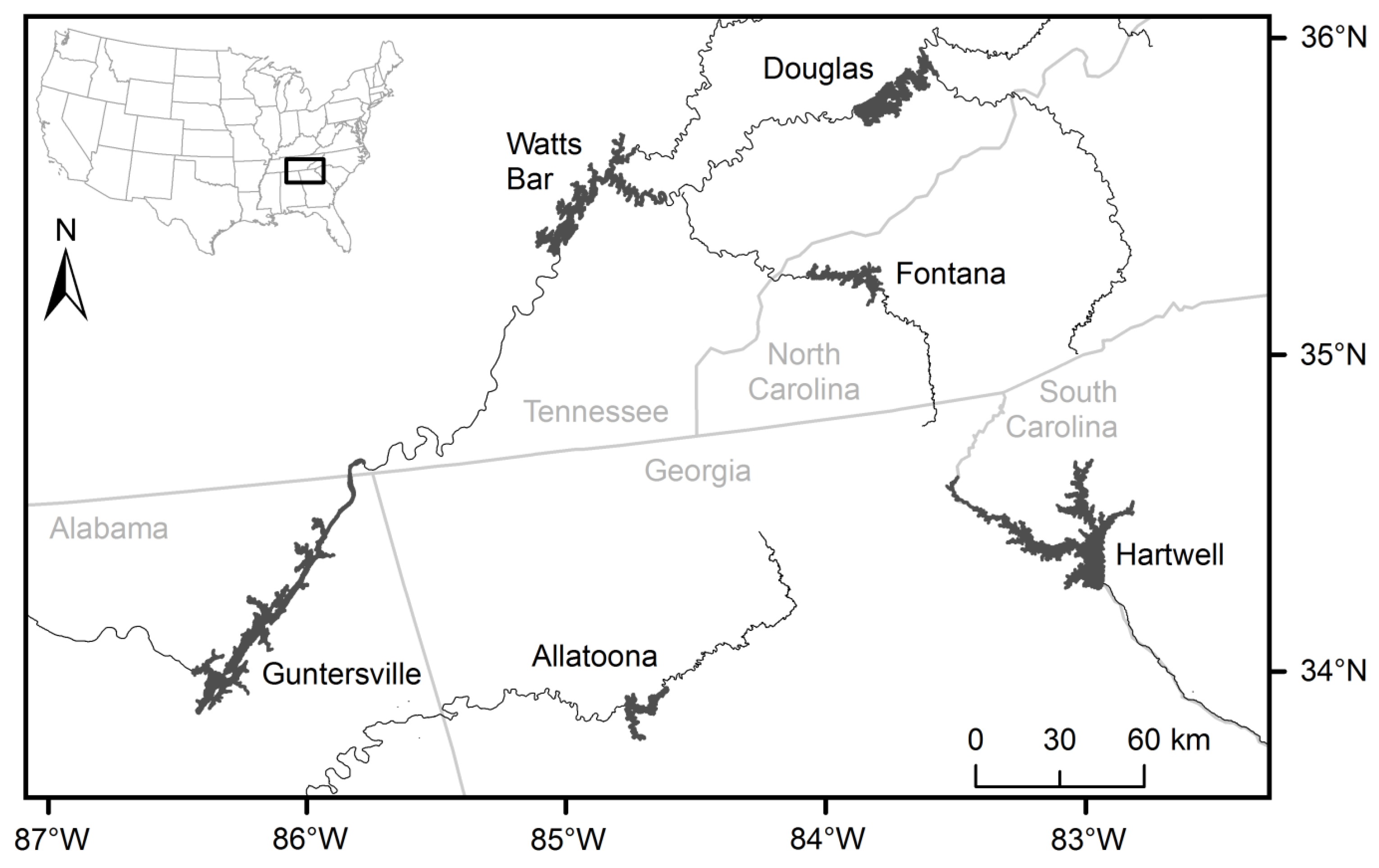
2.1. Study Sites

The 6 reservoirs represent a 5-state region in the U.S. southeast (Figure 1) and are generally of similar age (Hartwell is the youngest), but they range over about an order of magnitude in surface area, volume, depth, annual flow, and residence time (Table 1). All of these reservoirs are at relatively low elevation, but they vary significantly in the average amount of winter drawdown for flood storage purposes: Allatoona (full pool elevation 256 m msl; 5 m winter drawdown), Douglas (302 m msl, 13 m), Fontana (519 m msl, 16 m), Guntersville (181 m msl, 0.3 m), Hartwell (201 m msl, 1 m), and Watts Bar (226 m msl, 2 m).

Comprehensive sampling of water quality and emissions required two to three days per reservoir and was conducted from 20 August to 20 September 2012. Precipitation in the region during the previous 12 months was normal (~1% above the 120-year average) and mean temperature was slightly warmer (~1.5 °C above the long-term average) [31]. The summer months (June–August) of 2012 also had normal precipitation (within 10%) and temperature (within 1 °C) relative to long-term averages for those months.

Emissions sampling followed internationally developed protocol [32] at seven locations per reservoir; the locations included three main channel sites, three cove sites, and a tailwater site. Tailwaters were sampled at a distance of at least 500 m downstream of the turbine discharge as recommended for gas equilibration [32] at all sites except at Lake Hartwell, which was sampled at a distance of 300 m. The three main channel sites were spaced as evenly as practical along the length of the reservoir. Cove sites were randomly selected; some coves were fed by perennial streams and others were not. The specific locations (latitude and longitude) for each sample site are included in the Supplementary Materials (S1).

Figure 1. Locations of six southeastern U.S. hydropower reservoirs sampled for greenhouse gas emissions in 2012.

Figure 1. Locations of six southeastern U.S. hydropower reservoirs sampled for greenhouse gas emissions in 2012.

Table 1. Morphological and hydrological characteristics of six study reservoirs in the southeastern U.S.

Reservoir	Year Constructed	Surface Area (km2)	Percent Area in Coves	Volume (106 m3)	Mean Depth (m)	Shoreline Development Index 1	Mean Annual Flow (m3 s−1)	Residence Time (day)
Allatoona	1949	49	63	453	9.2	17.6	58	36
Douglas	1943	115	41	1334	11.6	22.6	254	91
Fontana	1944	43	44	1780	41.4	16.1	123	180
Guntersville	1939	279	49	1256	4.5	24.2	1397	14
Hartwell	1962	226	48	3145	13.9	29.0	161	56
Watts Bar	1942	176	46	1396	7.9	26.1	964	21

Note: ¹ Shoreline development (SLD) is an index of the regularity of the shoreline. $\text{SLD}=\text{S}/\left(2\sqrt{A\pi }\right)$ where S = length of shoreline and A = area of lake. A reservoir that is a perfect circle would have an SLD = 1; dendritic reservoirs or those with complex shorelines might have a much larger SLD value [33].

Table 1. Morphological and hydrological characteristics of six study reservoirs in the southeastern U.S.

Reservoir	Year Constructed	Surface Area (km2)	Percent Area in Coves	Volume (106 m3)	Mean Depth (m)	Shoreline Development Index 1	Mean Annual Flow (m3 s−1)	Residence Time (day)
Allatoona	1949	49	63	453	9.2	17.6	58	36
Douglas	1943	115	41	1334	11.6	22.6	254	91
Fontana	1944	43	44	1780	41.4	16.1	123	180
Guntersville	1939	279	49	1256	4.5	24.2	1397	14
Hartwell	1962	226	48	3145	13.9	29.0	161	56
Watts Bar	1942	176	46	1396	7.9	26.1	964	21

Note: ¹ Shoreline development (SLD) is an index of the regularity of the shoreline. $\text{SLD}=\text{S}/\left(2\sqrt{A\pi }\right)$ where S = length of shoreline and A = area of lake. A reservoir that is a perfect circle would have an SLD = 1; dendritic reservoirs or those with complex shorelines might have a much larger SLD value [33].

The collection location (main channel, cove, or tailwater) dictated which of three methods was used: direct measurement of diffusion with a floating dome at mainstem and cove sites; indirect measurement based on dissolved gas concentrations at all sites; and direct measurement of ebullition losses with inverted funnels at cove sites only.

2.2. Diffusive Emissions Measurements

We measured diffusive fluxes of CO₂ and CH₄ from the water surface at three main channel sites and three cove sites in each reservoir with a floating chamber (volume, 19.8 L; surface area, 0.2 m²), which had sidewalls extending about 5 cm below the water surface and 15 cm above the surface, as described in the IHA manual [32]. The chamber was positioned on the water surface at the sampling site, and concentrations of CO₂ and CH₄ were measured continuously in the chamber headspace with a field GHG analyzer (Los Gatos Research, Inc.; model number DLT 100-908-0011-0001) operating in continuous-flow mode during an incubation period of 10 to 15 min. The GHG analyzer was calibrated using analytical grade CH₄ (100 ppm in N₂) (Supelco #307300-U) and CO₂ (1000 ppm in N₂) (Supelco #501336) in a six point calibration curve (R² > 0.9) using 99.99% N₂ as a diluent in a series of 1-L, 2-L and 5-L Tedlar PLV gas sampling bags equipped with Thermogreen LB-2 septa. We used N₂ as a diluent for calibrations and for sample analysis in the lab and field.

During the incubation, the chamber was allowed to float and drift with the water current, but remained tethered to the GHG analyzer on the boat by tubing in a closed-loop arrangement. The concentrations of CO₂ and CH₄ in the chamber headspace, the surface area of the floating chamber, and the duration of the incubation period were used to calculate diffusive emissions from the slope of the increase in gas concentration over time (mg of CO₂ and mg of CH₄ m⁻²·day⁻¹; Equation (1)).

$$Flux\left(mg·m^{-2}·da{y}^{-1}\right)=\frac{slope\left(ppm·s^{-1}\right)\times F_1\times F_2\times chambervol\left(m^3\right)}{Chambersurface\left(m^2\right)}$$

(1)

where F₁ is a conversion factor from ppm to mg m⁻³ for standard temperature and pressure for gas in air (perfect gas formula), and F₂ is a conversion factor of seconds into days (24 h × 60 min × 60 s or 86,400 s·day⁻¹). Slope estimates with regression coefficients, R² < 0.75 were rejected.

Sampling for all gas measurements, whether by diffusion, ebullition, or dissolved gasses, were made during the day from 8:00 A.M. to 4:00 P.M. Because CO₂ concentrations are affected by daily cycles of plant photosynthesis and respiration, i.e., concentrations are typically highest in the morning and lowest in the evening, some effect of sampling time on flux is possible. Surface measurements of diffusion are more likely to be affected than dissolved gas measurements of water collected from depth. Unfortunately, because of the time it takes to collect samples and to move between sampling sites, it is not possible to control for this variable.

2.3. Measurements of Dissolved Gases in Water

Because sampling with a floating dome or inverted funnels is difficult in flowing water and because many tailwaters are not accessible by boat, our estimates of gas emissions from dam tailwaters were based on the difference between dissolved gas concentrations in the reservoir and the tailwater. In each reservoir, we used a Van Dorn sampler attached to a nylon rope to collect water samples at 1 m and 25 m depth (or within 1 m of the bottom when the depth was less than 25 m) at both cove and main channel sites. In each tailwater, the sampler was thrown or lowered from shore into the tailwaters during power generation periods, to obtain water samples. We measured the concentrations of dissolved CO₂ and CH₄ in these water samples using a headspace analysis method, as follows: a 70-mL volume of freshly collected water was withdrawn from the Van Dorn sampler using a 140-mL syringe. We then introduced 70 mL of N₂ into the syringe by a needle through a gas-tight septum on a sealed gas bag containing N₂. The contents of the syringe were mixed by shaking, and the 70 mL of water was expelled. The volume in the syringe was then reconstituted to 140 mL with additional N₂. The entire 140 mL gas sample was then analyzed for CO₂ and CH₄ with the Los Gatos GHG analyzer operating in injection mode. Corrections for solubility (as influenced by water temperature and salinity) were incorporated into the calculations for converting the measured gas concentrations into the dissolved-phase concentrations using equations in IHA [32].

2.4. Ebullition Measurements

Eight funnel samplers (four per cove, in each of two coves per reservoir) intercepted bubbles traveling to the surface, which were collected for characterizing CO₂ and CH₄ ebullition rates [32]. Coves were chosen for sampling over the main channel for logistic reasons (less boat traffic, shallower water depth, and slower currents) and because earlier sampling revealed that coves typically have greater ebullition rates than the main channel [29,30]. Inverted funnels of 1 m diameter opening (0.79 m² opening area) at approximately 1.5 m below the water surface collected gases overnight (15 to 28 h in 73 cases; but in 13 cases, funnels were deployed for up to 48 h due to storms that interfered with scheduled retrieval). For each funnel, the total volume of gases trapped was removed with a 140-mL syringe, and the remainder of the syringe was filled with pure nitrogen. The entire 140 mL of gas was then injected into the gas analyzer operating in injection mode. The total volume of gases collected in the syringe, the measured concentrations of CO₂ and CH₄ in subsamples of the gases in the syringe, the length of time the funnel was deployed, and the area sampled by the funnel (0.79 m²) were used to calculate CO₂ and CH₄ ebullition rates (mg CO₂ or mg CH₄ m⁻²·day⁻¹; Equation (2)) [32].

$$Bubblingflux\left(mg·m^{-2}·da{y}^{-1}\right)=\frac{gasconc\left(mg·m^{-3}\right)\times gasvolcollected\left(m^3\right)}{funnelarea\left(m^2\right)\times samplinginterval\left(day\right)}$$

(2)

2.5. Other Water Quality Factors

Concentrations of dissolved oxygen (DO), water temperature, conductivity, pH and chlorophyll a were measured at multiple depths at cove and channel sites in each reservoir using a Yellow Springs Instrument (YSI) model 650 MDS sonde. At each site, these depth-profile measurements were made at 0.1 m, 1 m, and at 2-m intervals thereafter (e.g., at 3 m, 5 m, 7 m, 9 m, etc.), either to maximum water depth or to 49 m, whichever came first. Maximum water depth (by sonar), water transparency (Secchi disk), and wind speed 1 m above the water surface and air temperature (by Kestrel model 4500 Pocket Weather Tracker) were also measured at each site.

2.6. Pathway Emissions Calculations

For diffusive emissions from the reservoir surface, we converted areal estimates of CO₂ and CH₄ emissions as shown in Equation (1) to reservoir-wide estimates by multiplying the mean per-square-meter emission rate times the reservoir surface area. For ebullitive emissions from the reservoir surface, we converted areal estimates of CO₂ and CH₄ emissions as shown in Equation (2) to reservoir-wide estimates by multiplying the mean per-square-meter emission rate times the cove portion of the reservoir surface area. Both total surface area and percent cove area can be found in Table 1.

Calculation of tailwater emissions is more complicated as gases are lost by two not entirely distinct modes as a result of hydropower generation. Degassing occurs first as water passes through the turbines, presumably at a higher rate if the turbines have aerating features. Then, as water that is high in dissolved gases continues downstream, gases continue to be emitted due to the turbulent nature of the flow until concentrations reach an equilibrium typical of water at the air-water interface. Standard protocol [32] suggest taking tailwater samples at least 500 m downstream of the turbine discharge in order to sample water that has had time to reach equilibrium. All but one of our samples were 500 m or more downstream, but it was apparent from the elevated levels at some sites that this was not enough for equilibrium to have been achieved.

Therefore, our estimate of gas emitted in the tailwater was the sum of two parts—first, an estimate of the amount of gas emitted from the deep reservoir source to the point of tailwater sample collection and, second, the amount emitted from the point of tailwater sampling to the theoretical point of equilibrium with the air. For the first estimate we subtracted the tailwater measurement from the mean of the three deep main channel samples (mg·L⁻¹) and multiplied the result times the average daily discharge (L·s⁻¹). All dams had deep water intakes, and in the absence of any consistent downstream pattern in gas concentrations among main channel sites, we presumed that the average of the three deep values at each reservoir was a reasonable representation of what passed through the turbines. For the second estimate we subtracted an estimate of the equilibrium concentration based on all sampling combined from the tailwater concentration (mg·L⁻¹) and multiplied the result times the average daily discharge (L·s⁻¹). The sum expressed as a single equation is

$$\begin{array}{l}Tailwateremissions\left(mg·da{y}^{-1}\right)\\ =(\left(\left[gasdeepreservoir\left(\mathsf{\mu }mol·L^{-1}\right)]-[gastailwaters\left(\mathsf{\mu }mol·L^{-1}\right)\right]\right)\\ +\left(\left[gastailwaters\left(\mathsf{\mu }mol·L^{-1}\right)]-[surfacewaterequilibrium\left(\mathsf{\mu }mol·L^{-1}\right)\right]\right))\\ \times F3\times discharge\left(L·da{y}^{-1}\right)\end{array}$$

(3)

where F₃ is a conversion factor from µmol·L⁻¹ to mg·L⁻¹ (0.04401 for CO₂ and 0.01601 for CH₄). The equilibrium values for CO₂ and CH₄ were estimated as the general mean of the lowest concentrations observed in water samples collected from the reservoir surface and the tailwaters, 25 µmol·L⁻¹ for CO₂ and 0.25 µmol·L⁻¹ for CH₄. This method of estimating tailwater emissions assumes no downstream non-atmospheric losses of dissolved CO₂ (e.g., to algae) or CH₄ (e.g., to methane-oxidizing bacteria), but we would not expect this to create a substantial overestimation of tailwater emissions.

3. Results

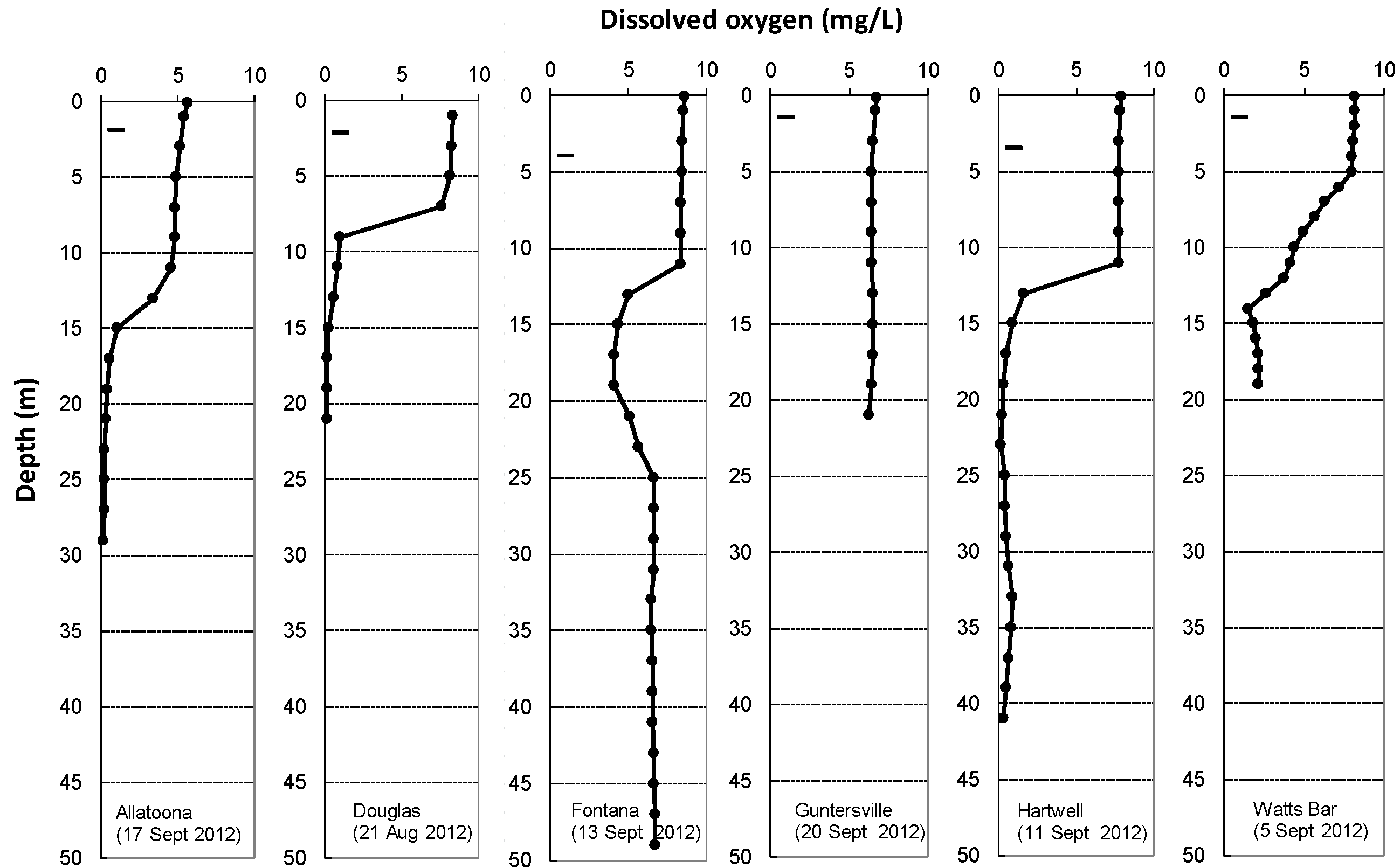
3.1. Water Quality and Wind Speed

Differences in water quality characteristics among reservoirs were largely correlated with vertical thermal stratification of the water column and reservoir productivity (Table 2). Surface-water temperatures (average of shallow-water depths in cove and channel sites) ranged from 20.3 °C for Allatoona to 28.0 °C for Douglas. Concentrations of DO at shallow (i.e., 0.1 and 1 m) depths exceeded 5 mg·L⁻¹ at all sites in all reservoirs, but we found low levels of DO (e.g., <2 mg·L⁻¹) at depths >15 m in Allatoona, >7 m in Douglas, >13 m in Hartwell, and >7 m at several sites in Watts Bar (Figure 2). In Fontana, all measured values of DO were >2 mg·L⁻¹. DO concentrations were 2.36–4.0 mg·L⁻¹ in Fontana at depths of 17 m to 45 m in several cove sites, but were > 4.0 mg·L⁻¹ at all other sites in Fontana, to a depth of 49 m (the maximum sampling depth). In Guntersville, DO concentrations were between 6.03 and 8.74 mg·L⁻¹ throughout (Figure 2). Anoxic areas of a reservoir are often more conducive to dissolved methane accumulation.

Table 2. Water quality measures and mean wind speed during sampling of gas emissions at six hydropower reservoirs in the southeastern U.S.

Reservoir	Profile Temperature Range (°C)	Profile DO Range (mg·L−1)	Mean Secchi Depth (m)	Mixed Layer Depth (m)	Mean Chlorophyll a (µg·L−1)	Mean Wind Speed (m·s−1)
Allatoona	17.9–26.6	0.2–6.6	1.92	15	4.4	2.0
Douglas	18.1–28.8	0.1–9.4	2.14	9	3.7	1.4
Fontana	12.5–26.3	2.4–8.6	3.95	13	5.9	1.0
Guntersville	20.8–26.5	6.0–8.7	1.37	all	1.8	1.5
Hartwell	11.4–28.5	0.2–8.2	3.43	13	9.5	1.9
Watts Bar	24.1–27.7	0.6–10.0	1.45	all	2.3	3.0

Table 2. Water quality measures and mean wind speed during sampling of gas emissions at six hydropower reservoirs in the southeastern U.S.

Reservoir	Profile Temperature Range (°C)	Profile DO Range (mg·L−1)	Mean Secchi Depth (m)	Mixed Layer Depth (m)	Mean Chlorophyll a (µg·L−1)	Mean Wind Speed (m·s−1)
Allatoona	17.9–26.6	0.2–6.6	1.92	15	4.4	2.0
Douglas	18.1–28.8	0.1–9.4	2.14	9	3.7	1.4
Fontana	12.5–26.3	2.4–8.6	3.95	13	5.9	1.0
Guntersville	20.8–26.5	6.0–8.7	1.37	all	1.8	1.5
Hartwell	11.4–28.5	0.2–8.2	3.43	13	9.5	1.9
Watts Bar	24.1–27.7	0.6–10.0	1.45	all	2.3	3.0

Figure 2. Vertical profiles of dissolved oxygen (mg·L⁻¹) for six southeastern U.S. reservoirs during synoptic sampling in late summer 2012. The single dash represents the Secchi disk depth. Data presented are from the deepest main channel site at each reservoir.

Figure 2. Vertical profiles of dissolved oxygen (mg·L⁻¹) for six southeastern U.S. reservoirs during synoptic sampling in late summer 2012. The single dash represents the Secchi disk depth. Data presented are from the deepest main channel site at each reservoir.

Water transparency (characterized as mean Secchi disk depth) varied about three-fold among the reservoirs. In Fontana, the mean Secchi disk depth was 4.13 m; in Guntersville 1.44 m; and for Hartwell, Douglas, Allatoona, and Watts Bar 3.59 m, 2.20 m, 1.93 m and 1.50 m, respectively (Table 2). Wind speeds measured during GHG measurements ranged from 0.5 to 3.6 m/s.

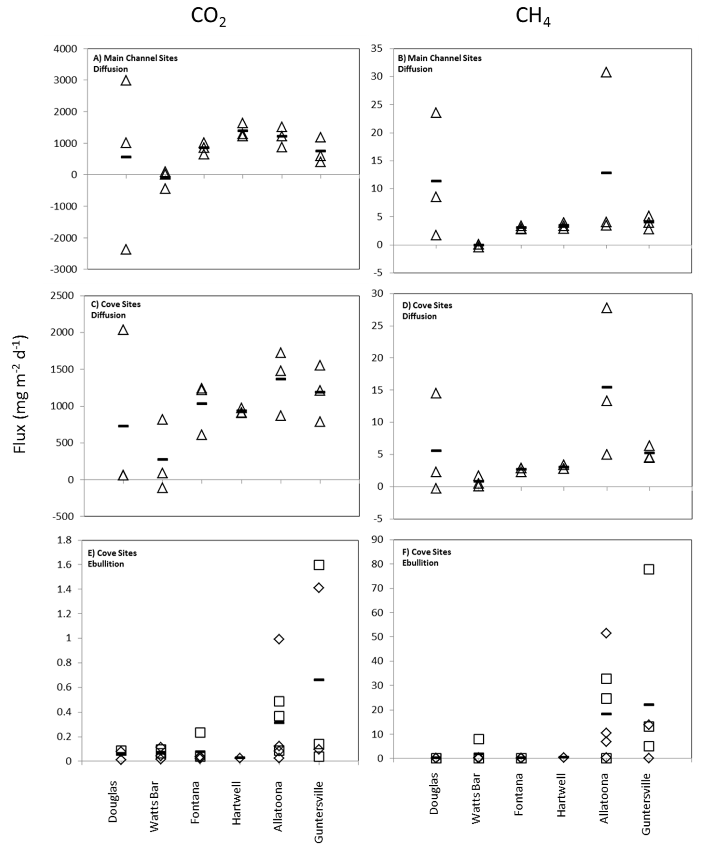
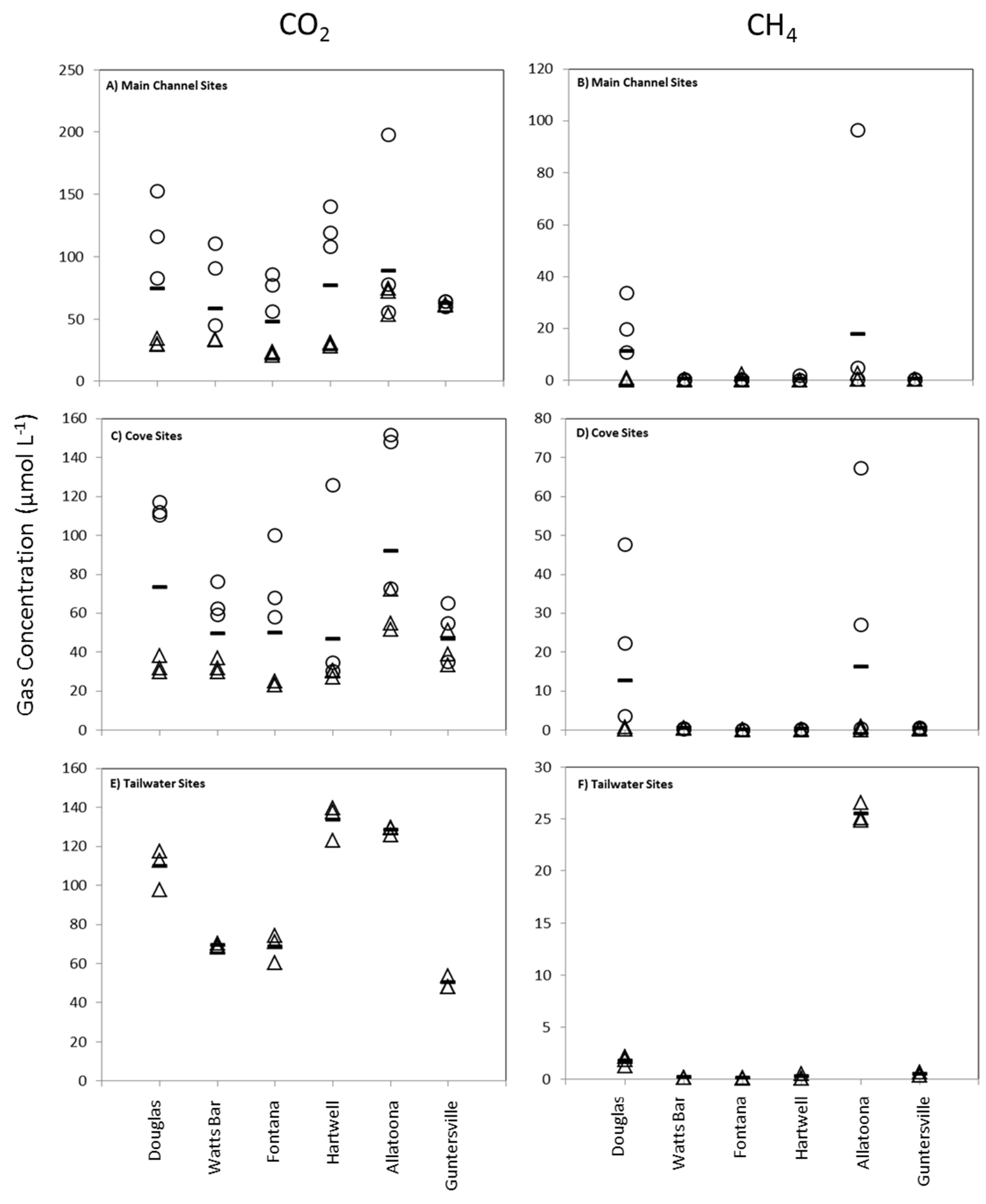
3.2. Gas Concentrations and Emission Rates

Flux of CO₂ measured as diffusion (dome measurements) was generally similar among reservoirs except that Watts Bar was consistently lower than the others (Figure 3A,C). The highest CH₄ flux by diffusion was measured at Allatoona and Douglas (Figure 3B,D). Flux of both CO₂ and CH₄ measured as ebullition (funnel measurements) was low for Douglas, Fontana, Hartwell, and Watts Bar compared to that at Allatoona and Guntersville (Figure 3E,F). A few measurements were negative, and most of these are likely the results of slight errors in measurement of emissions that were zero or near zero. However, in the case of CO₂ it is theoretically possible that a system with a high rate of photosynthesis could at times remove CO₂ from the atmosphere resulting in a negative flux.

Figure 3. Individual and mean flux measurements of CO₂ and CH₄ from six reservoirs by diffusion at main channel sites (A,B); diffusion at cove sites (C,D); and ebullition at cove sites (E,F). Triangles represent 20-min dome measurements. Diamonds and squares represent overnight funnel measurements at two coves. Mean values are indicated with a dash.

Figure 3. Individual and mean flux measurements of CO₂ and CH₄ from six reservoirs by diffusion at main channel sites (A,B); diffusion at cove sites (C,D); and ebullition at cove sites (E,F). Triangles represent 20-min dome measurements. Diamonds and squares represent overnight funnel measurements at two coves. Mean values are indicated with a dash.

Water concentrations of CO₂ and CH₄ (based on GC analysis of water samples) were generally higher in deeper samples at both main channel and cove sites (Figure 4A–D). Although variation among and within reservoirs was high, mean values of both gases at Allatoona and Douglas were generally higher than the other reservoirs. We did not find consistent upstream to downstream trends (neither increasing nor decreasing) in either CO₂ or CH₄ concentrations within reservoirs. In tailwaters, the highest values of CO₂ were found at Allatoona, Douglas, and Hartwell (Figure 4E), and for CH₄ the highest values were found at Allatoona (Figure 4F). As discussed earlier, the lowest water concentrations of CO₂ and CH₄ were used to estimate the generic water surface equilibrium values used in tailwater emissions calculations.

Figure 4. Concentrations (µmol·L⁻¹) of CO₂ and CH₄ from water samples collected from main channel (A,B), cove (C,D), and tailwater sites (E,F) at six reservoirs. Triangles represent samples from the surface (1 m depth) and circles represent samples collected 1 m above the bottom. Mean values are indicated with a dash.

Figure 4. Concentrations (µmol·L⁻¹) of CO₂ and CH₄ from water samples collected from main channel (A,B), cove (C,D), and tailwater sites (E,F) at six reservoirs. Triangles represent samples from the surface (1 m depth) and circles represent samples collected 1 m above the bottom. Mean values are indicated with a dash.

Estimates of total (i.e., whole-reservoir) daily releases of CO₂ and CH₄ from the six reservoirs, by diffusive, ebullition and tailwater pathways are summarized in Table 3. Diffusive emissions of CO₂ from the reservoirs exceeded CO₂ emissions in the tailwaters for Allatoona, Fontana, Guntersville, and Hartwell, but were less than tailwater losses for Douglas and Watts Bar reservoirs. Ebullitive emissions of CO₂ were minimal compared to the other two pathways. Releases of CH₄ via surface diffusion were greater than the other two pathways at Fontana, Hartwell, and Watts Bar; greatest via the tailwater pathway at Allatoona and Douglas; and highest by ebullition only at Guntersville. Allatoona had the highest total CH₄ emissions of the six reservoirs, and Fontana, the deepest reservoir and the one with the longest residence time, had the lowest total.

Table 3. Total CO₂ and CH₄ releases from six southeastern U.S. hydropower reservoirs through diffusive emission, ebullition, and tailwater pathways.

Reservoir	Diffusion (kg·day−1)	Ebullition (kg·day−1)	Tailwater (kg·day−1)	Total (kg·day−1)	Total (mg·m−2·day−1)
CO2
Allatoona	80,200	13	38,064	118,277	2414
Douglas	78,235	3	87,844	166,082	1444
Fontana	28,192	2	14,546	42,740	994
Guntersville	315,943	114	185,094	501,151	1796
Hartwell	213,013	6	50,844	263,863	1168
Watts Bar	172,422	8	313,372	485,802	2760
CH4
Allatoona	678	767	7708	9153	187
Douglas	874	0	3704	4578	40
Fontana	251	0	0	251	6
Guntersville	1495	3834	446	5775	21
Hartwell	5151	47	0	5198	23
Watts Bar	1156	170	0	1326	8

Table 3. Total CO₂ and CH₄ releases from six southeastern U.S. hydropower reservoirs through diffusive emission, ebullition, and tailwater pathways.

Reservoir	Diffusion (kg·day−1)	Ebullition (kg·day−1)	Tailwater (kg·day−1)	Total (kg·day−1)	Total (mg·m−2·day−1)
CO2
Allatoona	80,200	13	38,064	118,277	2414
Douglas	78,235	3	87,844	166,082	1444
Fontana	28,192	2	14,546	42,740	994
Guntersville	315,943	114	185,094	501,151	1796
Hartwell	213,013	6	50,844	263,863	1168
Watts Bar	172,422	8	313,372	485,802	2760
CH4
Allatoona	678	767	7708	9153	187
Douglas	874	0	3704	4578	40
Fontana	251	0	0	251	6
Guntersville	1495	3834	446	5775	21
Hartwell	5151	47	0	5198	23
Watts Bar	1156	170	0	1326	8

3.3. Reservoir-Wide Emissions

Because reservoir-wide estimates of emissions were calculated as functions of either reservoir area (for diffusion and ebullition) or mean annual river flow (for tailwater emissions) the largest reservoirs and those with greatest flows had the highest total reservoir emissions of CO₂ (Guntersville, Hartwell, and Watts Bar). This was not the case with CH₄ where differences among reservoirs in areal estimates of emissions were greater than differences in size.

3.4. Contributing Factors

A Pearson correlation analysis was performed to evaluate associations between CO₂ and CH₄ emissions (three pathways and total for both) and various metrics of reservoir morphology and water-quality (Table 4). Correlations with r values > 0.73 or < −0.73 were considered to be significant (two-tailed, n = 6, level of significance = 0.1). The results suggest that reservoirs with higher maximum DO levels have lower diffusive CO₂ emissions, as do those reservoirs that have a larger proportion of their overall area as main channel (i.e., less off-channel cove area). High emission of CO₂ in the tailwaters was positively correlated with minimum temperature (an indicator of strength of the thermal stratification), and total CO₂ emissions (all pathways combined) correlated positively with minimum temperature and negatively with water transparency (i.e., Secchi disk depth). Surface diffusion of CH₄ was positively correlated with chlorophyll a, while CH₄ ebullition was negatively correlated with percent main channel area. Both tailwater emissions and total emissions of CH₄ were negatively correlated with maximum DO and percent main channel area.

Table 4. Pearson correlation coefficients between areal emissions of CO₂ and CH₄ (mg·m⁻²·day⁻¹) by diffusion, ebullition, and tailwater pathways and selected properties of the hydropower reservoirs. Significant correlations (−0.73 > r > 0.73) are indicated by bold font [34].

Parameter	CO2 Diffusion	CO2 Ebullition	CO2 Tailwater	CO2 Total	CH4 Diffusion	CH4 Ebullition	CH4 Tailwater	CH4 Total
Minimum temperature	0.28	0.36	0.89	0.84	-0.57	0.32	0.06	0.03
Maximum temperature	−0.39	−0.63	0.09	−0.13	0.41	−0.60	−0.24	−0.24
Minimum DO	0.00	0.72	−0.17	−0.13	−0.50	0.43	−0.35	−0.32
Maximum DO	−0.73	−0.43	0.50	0.02	−0.50	−0.65	−0.78	−0.83
Secchi depth	−0.48	−0.55	−0.71	−0.80	0.37	−0.54	−0.24	−0.24
Mean chlorophyll a	−0.18	−0.50	−0.68	−0.62	0.83	−0.41	−0.07	−0.03
Surface area	−0.02	0.32	0.06	0.04	0.13	0.08	−0.55	−0.47
Percent main channel by area	−0.97	−0.61	0.01	−0.49	−0.33	−0.84	−0.83	−0.88
Volume	−0.52	−0.53	−0.45	−0.62	0.58	−0.64	−0.65	−0.60
Mean depth	−0.53	−0.44	−0.46	−0.63	−0.14	−0.47	−0.23	−0.28
Shoreline development index	−0.10	0.10	0.05	−0.01	0.31	−0.10	−0.57	−0.49
Mean annual flow	−0.13	−0.16	0.19	0.08	0.41	−0.28	−0.50	−0.44
Residence time	0.06	0.54	0.47	0.40	−0.51	0.29	−0.43	−0.41

Table 4. Pearson correlation coefficients between areal emissions of CO₂ and CH₄ (mg·m⁻²·day⁻¹) by diffusion, ebullition, and tailwater pathways and selected properties of the hydropower reservoirs. Significant correlations (−0.73 > r > 0.73) are indicated by bold font [34].

Parameter	CO2 Diffusion	CO2 Ebullition	CO2 Tailwater	CO2 Total	CH4 Diffusion	CH4 Ebullition	CH4 Tailwater	CH4 Total
Minimum temperature	0.28	0.36	0.89	0.84	-0.57	0.32	0.06	0.03
Maximum temperature	−0.39	−0.63	0.09	−0.13	0.41	−0.60	−0.24	−0.24
Minimum DO	0.00	0.72	−0.17	−0.13	−0.50	0.43	−0.35	−0.32
Maximum DO	−0.73	−0.43	0.50	0.02	−0.50	−0.65	−0.78	−0.83
Secchi depth	−0.48	−0.55	−0.71	−0.80	0.37	−0.54	−0.24	−0.24
Mean chlorophyll a	−0.18	−0.50	−0.68	−0.62	0.83	−0.41	−0.07	−0.03
Surface area	−0.02	0.32	0.06	0.04	0.13	0.08	−0.55	−0.47
Percent main channel by area	−0.97	−0.61	0.01	−0.49	−0.33	−0.84	−0.83	−0.88
Volume	−0.52	−0.53	−0.45	−0.62	0.58	−0.64	−0.65	−0.60
Mean depth	−0.53	−0.44	−0.46	−0.63	−0.14	−0.47	−0.23	−0.28
Shoreline development index	−0.10	0.10	0.05	−0.01	0.31	−0.10	−0.57	−0.49
Mean annual flow	−0.13	−0.16	0.19	0.08	0.41	−0.28	−0.50	−0.44
Residence time	0.06	0.54	0.47	0.40	−0.51	0.29	−0.43	−0.41

3.5. Global Warming Potential

Because the relative emissions of CO₂ and CH₄ are not consistent among pathways, we calculated total global warming potential (TGWP) in CO₂ equivalents for gases emitted from the reservoir (combining diffusion and ebullition) and the tailwaters separately by adding total CO₂ emissions to 21 × total CH₄ emissions [35]. The ratio of reservoir TGWP to tailwater TGWP ranged from 0.4 to 7.6 (Douglas 0.4, Watts Bar 1.1, Allatoona 1.4, Fontana 1.5, Guntersville 2.2, and Hartwell 7.6). Note that a ratio of 1 means that the reservoir and tailwater contribute equal amounts to TGWP, a ratio of 2 means the reservoir contributes twice as much, and so on.

4. Discussion

The goal of this study was to sample GHG emissions at multiple hydropower reservoirs over the southeastern U.S. during a 1–2 month period when emissions are expected to be at an annual peak. Logistics associated with equipment costs and availability, transportation among reservoirs and sampling sites, and the time to collect and process samples, meant that our sampling had to be limited to what was necessary to develop an approximation of reservoir emissions. We found a great deal of variability among sites that suggests that there is substantial spatial heterogeneity. Although more sample sites per reservoir and more samples collected per site would have minimized the effect of among-site differences in various environmental factors (e.g., wind-speed, depth, local allochthonous input, vegetation, etc.) and could have provided more statistical rigor, we believe that the balance we struck between number of reservoirs, number of samples, and minimizing the sampling period provided the necessary data to compare emissions among the six sites and with other regions around the world.

An additional source of variability that we could not easily account for was time of day differences in emissions. Natural diel cycles of CO₂ consumption and production by photosynthesis and respiration likely produce some diel variation in CO₂ emissions. Our sampling took place from 8:00 A.M. to 5:00 P.M. and did not account for possible diel variation in GHG emissions. Therefore, results presented in this study are for diffusive emissions during daytime and do not necessarily represent the average emission over a full 24 h period.

It should also be noted that because these data were purposely collected during a period of peak emissions (August–September), the values in this study should not be considered to be averages applicable throughout the year. Areal estimates should be considered to be near the maximum rates during the year, as should the total reservoir pool estimates. Tailwater estimates were based on the mean annual daily flow rate through the dam which should be similar to the mean daily flow rate since these projects operate on a fairly consistent basis all year round.

Globally, Barros et al. [8] reported that most hydropower reservoirs between 68° N and 25° S were sources of CO₂ to the atmosphere, with total emission rates ranging from near zero to about 7300 mg CO₂ m⁻²·day⁻¹. The six reservoirs we investigated here also emitted CO₂, at rates ranging from about 1127 mg·m⁻²·day⁻¹ to 2051 mg·m⁻²·day⁻¹ (Table 3). Remember that our samples were purposefully collected during the summer period of peak emissions and the annual average would be less than what is reported here. The emission rates we measured also are within or near the ranges of values reported for multiple reservoirs cited by St. Louis et al. [36] and within the ranges of values for reservoirs in Manitoba, Ontario, and Quebec (980–3300 mg·m⁻²·day⁻¹) [9], northern California (1026–1247 mg·m⁻²·day⁻¹) [15], Finland (484–3212 mg·m⁻²·day⁻¹) [24], and Quebec (892–6703 mg·m⁻²·day⁻¹) [2]. The CO₂ diffusive emissions rates that we measured (656–1637 mg·m⁻²·day⁻¹) were lower than rates for a young reservoir in northern Quebec (1760–14,200 mg·m²·day⁻¹) [11] and much lower than for a tropical reservoir (7920–18,260 mg·m²·day⁻¹) [37].

Many hydropower reservoirs also have been reported to be CH₄ emitters [8,10,15,29,36,38]. We report CH₄ emission rates ranging from 5 mg·m²·day⁻¹ at Fontana to 77 mg·m⁻²·day⁻¹ at Allatoona and Douglas (Table 3). Compared to values of 20 mg·m⁻²·day⁻¹ reported by Saint Louis et al. [36] for reservoirs in temperate regions, the reservoirs sampled in this study range from relatively low to relatively high CH₄ emissions for temperate reservoirs. Compared to tropical reservoirs the reservoirs we sampled have much lower emission rates than tropical reservoirs [39].

Younger reservoirs with access to large stores of flooded vegetation appear to emit more CO₂ than older reservoirs [36]. The low emissions rates of CO₂ that we found (average of 1592 mg·m⁻²·day⁻¹ over the six reservoirs) may be due to the fact that the reservoirs we studied are relatively old (ages ranged from 50 years for Hartwell, to 74 years for Guntersville). As they have aged, the CO₂ and CH₄ production in these reservoirs has transitioned from mostly autochthonous origin to allochthonous and thus become more reflective of their catchments. From such considerations, we suggest that eutrophic reservoirs such as Guntersville and unusually oligotrophic southeast hydropower reservoirs such as Fontana may reasonably span the range for CO₂ emission rates for other hydropower reservoirs in southeastern U.S.

Two of the reservoirs we sampled (i.e., Douglas and Watts Bar) have forebay aeration systems designed to increase DO levels in dam tailwaters by increasing oxygen concentrations prior to turbine passage. These systems inject pure oxygen through bottom-mounted diffuser hoses creating streams of bubbles that partly go into solution as they rise to the surface. How these systems affect concentrations of CO₂ and CH₄ is largely unknown. The concentrations of CO₂ and CH₄ would likely be affected by one of two mechanisms or both. It is possible that O₂ bubbles might remove some dissolved CO₂ and CH₄ and deliver it to the surface where it is emitted from the reservoirs. Alternately, the increased oxygen in the water might enhance CH₄ oxidation thereby decreasing CH₄ concentrations and eventual emissions. If the former occurs then our method of calculations of total emissions from the reservoir would still be accurate. If on the other hand, forebay aeration causes increased CH₄ oxidation then our method would overestimate CH₄ emissions and slightly underestimated CO₂ emissions since the oxidation would increase CO₂ concentrations.

With only six data points it is difficult to provide definitive explanations about the significant correlations observed between reservoir fluxes and reservoir characteristics or water quality (Table 4). Minimum temperature and DO are indicators in the summer of the strength of vertical stratification, and can indicate that hypolimnetic conditions are anoxic enough to favor methane and gas bubble production. Maximum DO, transparency (i.e., Secchi depth), and chlorophyll a provide indications of general reservoir productivity and respiration. For total reservoir emissions, the largest reservoirs generally produce more GHG, but on a per square meter basis it appears that smaller-volume reservoirs produce more CO₂.

Expressed as a percentage of total CO₂ emissions, total CH₄ emissions were 0.5% for Fontana, 0.4% for Watts Bar, 0.5% for Douglas, 1.2% for Guntersville, 2.1% for Hartwell and 4.0% for Allatoona. The average total methane emissions in our study, expressed as a percentage of average total CO₂ emissions, was 2.2%. This value is similar to the value 1.3% calculated for average fluxes of CH₄ compared to CO₂ for temperate reservoirs, according to Table 2 in Saint Louis et al. [36].

DelSontro et al. [19] reported a strong positive correlation between water temperature and concentrations of dissolved methane in a Swiss hydropower reservoir, with total CH₄ emission rates of >150 mg·m⁻²·day⁻¹ being noted as very high for a mid-latitude reservoir. Campeau and Del Giorgio [1] also identified temperature as an important factor in CH₄ dynamics in streams and rivers in northern Quebec, Canada. The average total CH₄ emission rate in our study was much lower (28 mg·m⁻²·day⁻¹), and our study was done when surface temperatures should have been near annual maximum. Thus, we feel confident in suggesting that total emissions of CH₄ from most hydropower reservoirs in southeast U.S. are probably <5% of total CO₂ emissions, and possibly lower than 1%–2% of total CO₂ emissions, on an annual basis.

While total CH₄ emissions were low overall compared to the rates of total CO₂ emissions, CH₄ emissions by ebullition were large compared to CO₂ emissions by ebullition. For example, four of the six reservoirs had measurable levels of CH₄ ebullition, and for these reservoirs CH₄ ebullition exceeded CO₂ ebullition by ~8-fold (for Hartwell) to ~59-fold (for Allatoona). Ebullition as the primary source of CH₄ emissions is common [36].

Interestingly, total emissions of CH₄ and CH₄ emissions by ebullition from Guntersville were greater than for any of the other reservoirs, yet measured levels of DO for Guntersville were > 6 mg·L⁻¹ at all locations and sampling depths. Guntersville also was one of the shallower reservoirs (mean depth, 4.2 m), and had the lowest mean Secchi value (1.44 m) and had moderately high levels of chlorophyll a (mean, 6.58 µg·L⁻¹; range of means among all reservoirs was 1.52 µg·L⁻¹ for Fontana to 7.75 µg·L⁻¹ for Douglas).

We speculate that the large amounts of submersed and floating-leaved aquatic vegetation in Guntersville [40] may have accounted for both its high levels of CH₄ emissions and moderately high (>6 mg·L⁻¹) concentrations of DO. Submersed and floating-leaved vegetation can drive DO to very low levels at night and could also account for high levels of DO during the day (Guntersville was sampled 2.2–6.7 h after sunrise on 20 September), even as CH₄ production remained high due to organic-rich anoxic sediments. Further, aquatic plants can transport gases from the sediments to the surface [41,42,43]. The high rates of methane ebullition from Guntersville compared to CH₄ ebullition at the other reservoirs (Table 3) also support such possibility, because the funnel samplers integrated bubble-emissions over ~24-h periods. Based on recent evidence of high within-reservoir spatial variability in ebullition [44], we suggest that an intensive seasonal and diel sampling effort of GHG emissions with increased spatial coverage at Guntersville would be very informative on processes related to CH₄ and CO₂ ebullitive emissions from hydropower reservoirs.

The size, age and maximum depth of the reservoirs sampled in this study are representative of the range of hydropower reservoirs in the U.S. southeast, however, compared to hydropower reservoirs around the world these would be considered relatively old, small, and shallow. The data we present here add more understanding on GHG emissions from a small subset of a very large and diverse population of hydropower reservoirs across the world.

References

1. Campeau, A.; del Giorgio, P.A. Patterns in CH4 and CO2 concentrations across boreal rivers: Major drivers and implications for fluvial greenhouse emissions under climate change scenarios. Glob. Chang. Biol. 2014, 20. [Google Scholar] [CrossRef]
2. Tadonléké, R.D.; Marty, J.; Planas, D. Assessing factors underlying variation of CO2 emissions in boreal lakes vs. reservoirs. FEMS Microbiol. Ecol. 2012, 79. [Google Scholar] [CrossRef] [PubMed]
3. Kosten, S.; Roland, F.; da Motta Marques, D.M.L.; van Nes, E.H.; Mazzeo, N.; Sternberg, L.; Scheffer, M.; Cole, J.J. Climate-dependent CO2 emissions from lakes. Glob. Biogeochem. Cycles 2010, 24. [Google Scholar] [CrossRef]
4. Tranvik, L.J.; Downing, J.A.; Cotner, J.B.; Loiselle, S.A.; Striegl, R.G.; Ballatore, T.J.; Dillon, P.; Finlay, K.; Fortino, K.; Knoll, L.B.; et al. Lakes and reservoirs as regulators of carbon cycling and climate. Limnol. Oceanogr. 2009, 54. [Google Scholar] [CrossRef]
5. Bergström, A.K.; Algesten, G.; Sobek, S.; Tranvik, L.; Jansson, M. Emission of CO2 from hydroelectric reservoirs in northern Sweden. Arch. Hydrobiol. 2004, 159. [Google Scholar] [CrossRef]
6. Duarte, C.M.; Prairie, Y.T. Prevalence of heterotrophy and atmospheric CO2 emissions from aquatic ecosystems. Ecosystems 2005, 8. [Google Scholar] [CrossRef]
7. Failer, E.; El-Hadari, M.H.; Mutaz, M.A.S. The Merowe Dam and its hydropower plant in Sudan. Wasserwirtschaft 2011, 101, 10–16. [Google Scholar] [CrossRef]
8. Barros, N.; Cole, J.J.; Tranvik, L.J.; Prairie, Y.T.; Bastviken, D.; Huszar, V.L.M.; del Giorgio, P.; Roland, F. Carbon emission from hydroelectric reservoirs linked to reservoir age and latitude. Nat. Geosci. 2011, 4. [Google Scholar] [CrossRef]
9. Tremblay, A.; Lambert, M.; Gagnon, L. Do hydroelectric reservoirs emit greenhouse gases? Environ. Manag. 2004, 33. [Google Scholar] [CrossRef]
10. Galy-Lacaux, C.; Delmas, R.; Kouadio, G.; Richard, S.; Gosse, P. Long-term greenhouse gas emissions from hydroelectric reservoirs in tropical forest regions. Glob. Biogeochem. Cycles 1999, 13. [Google Scholar] [CrossRef]
11. Teodoru, C.R.; Prairie, Y.T.; del Giorgio, P.A. Spatial heterogeneity of surface CO2 fluxes in a newly created Eastmain-1 Reservoir in Northern Quebec, Canada. Ecosystems 2011, 14. [Google Scholar] [CrossRef]
12. Sobek, S.; Algesten, G.; Bergström, A.; Jansson, M.; Tranvik, L.J. The catchment and climate regulation of pCO2 in boreal lakes. Glob. Chang. Biol. 2003, 9. [Google Scholar] [CrossRef]
13. Sobek, S.; Tranvik, L.J.; Cole, J.J. Temperature independence of carbon dioxide supersaturation in global lakes. Glob. Biogeochem. Cycles 2005, 19. [Google Scholar] [CrossRef]
14. Trolle, D.; Staehr, P.A.; Davidson, T.A.; Bjerring, R.; Lauridsen, T.L.; Sondergaard, M.; Jeppesen, E. Seasonal dynamics of CO2 flux across the surface of shallow temperate lakes. Ecosystems 2012, 15, 336–347. [Google Scholar] [CrossRef]
15. Soumis, N.; Duchemin, E.; Canuel, R.; Lucotte, M. Greenhouse gas emissions from reservoirs of the western United States. Glob. Biogeochem. Cycles 2004, 18. [Google Scholar] [CrossRef]
16. Borrel, G.; Jezequel, D.; Biderre-Petit, C.; Morel-Desrosiers, N.; Morel, J.; Peyret, P.; Fonty, G.; Lehours, A. Production and consumption of methane in freshwater lake ecosystems. Res. Microbiol. 2011, 162. [Google Scholar] [CrossRef] [PubMed]
17. Bastviken, D.; Cole, J.J.; Pace, M.; Tranvik, L. Methane emissions from lakes: Dependence of lake characteristics, two regional assessments, and a global estimate. Glob. Biogeochem. Cycles 2004, 18. [Google Scholar] [CrossRef]
18. Rich, P.H.; Wetzel, R.G. Detritus in the lake ecosystem. Am. Nat. 1978, 112, 57–71. [Google Scholar] [CrossRef]
19. DelSontro, T.; McGinnis, D.F.; Sobek, S.; Ostrovsky, I.; Wehrli, B. Extreme methane emissions from a Swiss hydropower reservoir: Contribution from bubbling sediments. Environ. Sci. Technol. 2010, 44, 2419–2425. [Google Scholar] [CrossRef] [PubMed]
20. Ostrovsky, I.; Tegowski, J. Hydroacoustic analysis of spatial and temporal variability of bottom sediment characteristics in Lake Kinneret in relation to water level fluctuation. Geo-Mar. Lett. 2003, 30, 261–269. [Google Scholar] [CrossRef]
21. Murase, J.; Sakai, Y.; Sugimoto, A.; Okubo, K.; Sakamoto, M. Sources of dissolved methane in Lake Biwa. Limnology 2003, 4. [Google Scholar] [CrossRef]
22. Kelly, C.A.; Rudd, J.W.M.; Bodaly, R.A.; Roulet, N.P.; St. Louis, V.L.; Heyes, A.; Moore, T.R.; Schiff, S.; Aravena, R.; Scott, K.J.; et al. Increases in fluxes of greenhouse gases and methyl mercury following flooding of an experimental reservoir. Environ. Sci. Technol. 1997, 31. [Google Scholar] [CrossRef]
23. Matthews, D.A.; Effler, S.W.; Matthews, C.M. Long-term trends in methane flux from the sediments of Onondaga Lake, NY: Sediment diagenesis and impacts on dissolved oxygen resources. Arch. Hydrobiol. 2005, 163. [Google Scholar] [CrossRef]
24. Huttunen, J.T.; Alm, J.; Liikanen, A.; Juutinen, S.; Larmola, T.; Hammar, T.; Silvola, J.; Martikainen, P.J. Fluxes of methane, carbon dioxide and nitrous oxide in boreal lakes and potential anthropogenic effects on the aquatic greenhouse gas emissions. Chemosphere 2003, 52. [Google Scholar] [CrossRef]
25. Casper, P.; Maberly, S.C.; Hall, G.H.; Finlay, B.J. Fluxes of methane and carbon dioxide from a small productive lake to the atmosphere. Biogeochemistry 2000, 49. [Google Scholar] [CrossRef]
26. Goldenfum, J.A. Challenges and solutions for assessing the impact of freshwater reservoirs on natural GHG emissions. Ecohydrol. Hydrobiol. 2012, 12. [Google Scholar] [CrossRef]
27. Tremblay, A.; Varfalvy, L.; Roehm, G.; Garneau, M. Greenhouse Gas Emissions—Fluxes and Processes: Hydroelectric Reservoirs and Natural Environments; Springer: Berlin, Germany, 2005. [Google Scholar]
28. Beaulieu, J.J.; Smolenski, R.L.; Nietch, C.T.; Townsend-Small, A.; Elovitz, M.S. High methane emissions from a midlatitude reservoir draining an agricultural watershed. Environ. Sci. Technol. 2014, 48. [Google Scholar] [CrossRef] [PubMed]
29. Stewart, A.J.; Mosher, J.J.; Mulholland, P.J.; Fortner, A.M.; Phillips, J.R.; Bevelhimer, M.S. Greenhouse Gas Emissions from U.S. Hydropower Reservoirs: FY2011 Annual Progress Report; ORNL/TM-2012/90; Department of Energy: Washington, DC, USA, 2011.
30. Mosher, J.J.; Fortner, A.M.; Phillips, J.R.; Bevelhimer, M.S.; Stewart, A.J.; Troia, M.J. Spatial and temporal correlates of greenhouse gas diffusion from a hydropower reservoir in the southern United States. Water 2015, 7, 5910–5927. [Google Scholar] [CrossRef]
31. The Southeast Regional Climate Center. Monthly and Seasonal Climate Information. Available online: http://www.sercc.com/climateinfo/monthly_seasonal (accessed on 4 January 2016).
32. Goldenfum, J.A. GHG Measurement Guidelines for Freshwater Reservoirs; The International Hydropower Association: London, UK, 2010; Available online: http://www.hydropower.org/sites/default/files/publications-docs/GHG%20Measurement%20Guidelines%20for%20Freshwater%20Reservoirs.pdf (accessed on 4 January 2016).
33. Wetzel, R.G. Limnology: Lake and River Ecosystems, 3rd ed.; Academic Press: San Diego, CA, USA, 2001. [Google Scholar]
34. Zar, J.H. Biostatistical Analysis, 2nd ed.; Prentice-Hall, Inc.: Englewood Cliffs, NJ, USA, 1984. [Google Scholar]
35. Lelieveld, J.; Crutzen, P.J.; Dentener, F.J. Changing concentration, lifetime and climate forcing of atmospheric methane. Tellus B 1998, 50. [Google Scholar] [CrossRef]
36. St. Louis, V.L.; Kelly, C.A.; Duchemin, E.; Rudd, J.W.M.; Rosenberg, D.M. Reservoir surfaces as sources of greenhouse gases to the atmosphere: A global estimate. BioScience 2000, 50, 766–775. [Google Scholar] [CrossRef]
37. Kemenes, A.; Forsberg, B.R.; Melack, J.M. CO2 emissions from a tropical hydroelectric reservoir (Balbina, Brazil). J. Geophys. Res. 2011, 116. [Google Scholar] [CrossRef]
38. Duchemin, E.; Lucotte, M.; Canuel, R.; Chamberland, A. Production of greenhouse gases CH4 and CO2 by hydroelectric reservoirs of the boreal region. Glob. Biogeochem. Cycles 1995, 9. [Google Scholar] [CrossRef]
39. DelSontro, T.; Kunz, M.J.; Kempter, T.; Wüest, A.; Wehrli, B.; Senn, D.B. Spatial heterogeneity of methane ebullition in a large tropical reservoir. Environ. Sci. Technol. 2011, 45. [Google Scholar] [CrossRef] [PubMed]
40. Webb, D.H.; Mangum, L.N.; Bates, A.L.; Murphy, H.D. Aquatic vegetation in Guntersville reservoir following grass carp stocking. In Proceedings of the Grass Carp Symposium, Gainesville, FL, USA, 7–9 March 1994.
41. Dacey, J.W.H. Pressurized ventilation in the yellow waterlily. Ecology 1981, 62, 1137–1147. [Google Scholar] [CrossRef]
42. Lindberg, S.E.; Dong, W.; Chanton, J.; Qualls, R.G.; Meyers, T. A mechanism for bimodal emission of gaseous mercury from aquatic macrophytes. Atmos. Environ. 2005, 39, 1289–1301. [Google Scholar] [CrossRef]
43. Ribaudo, C.; Bartoli, M.; Longhi, D.; Castaldi, S.; Neubauer, S.C.; Viaroli, P. CO2 and CH4 fluxes across a Nuphar lutea (L.) Sm. stand. J. Limnol. 2012, 71, 200–210. [Google Scholar] [CrossRef]
44. DelSontro, T.; McGinnis, D.F.; Wehrli, B.; Ostrovsky, I. Size does matter: Importance of large bubbles and small-scale hot spots for methane transport. Environ. Sci. Technol. 2015, 49. [Google Scholar] [CrossRef] [PubMed]