Quantifying Rainfall Interception Loss of a Subtropical Broadleaved Forest in Central Taiwan

Abstract

The factors controlling seasonal rainfall interception loss are investigated by using a double-mass curve analysis, based on direct measurements of high-temporal resolution gross rainfall, throughfall and stemflow from 43 rainfall events that occurred in central Taiwan from April 2008 to April 2009. The canopy water storage capacity for the wet season was estimated to be 1.86 mm, about twice that for the dry season (0.91 mm), likely due to the large reduction in the leaf area index (LAI) from 4.63 to 2.23 (m²·m⁻²). Changes in seasonal canopy structure and micro-meteorological conditions resulted in temporal variations in the amount of interception components, and rainfall partitioning into stemflow and throughfall. Wet canopy evaporation after rainfall contributed 41.8% of the wet season interception loss, but only 17.1% of the dry season interception loss. Wet canopy evaporation during rainfall accounted for 82.9% of the dry season interception loss, but only 58.2% of the wet season interception loss. Throughfall accounted for over 79.7% of the dry season precipitation and 76.1% of the wet season precipitation, possibly due to the change in gap fraction from 64.2% in the dry season to 50.0% in the wet season. The reduced canopy cover in the dry season also produced less stemflow than that of the wet season. The rainfall stemflow ratio ($P_{sf}/P_g$) was reduced from 12.6% to 8.9%. Despite relatively large changes in canopy structure, seasonal variation of the ratio of rainfall partitioned to interception was quite small. Rainfall interception loss accounted for nearly 12% of gross precipitation for both dry and wet seasons.

1. Introduction

Quantifying the partitioning of gross rainfall ($P_g$) into interception loss (I) is very important for studying the water balance in surface hydrology, especially in forest hydrology. Here, I is the amount of precipitation that is intercepted, stored and subsequently evaporates from the canopy so produces fast feedback to the atmospheric rainfall and does not participate in the surface hydrological cycle. As one evapotranspiration component, the amount of interception loss not only changes the partitioning of $P_g$ into throughtfall ($P_{tf}$) and stemflow ($P_{sf}$) but influences the nutrient flux dynamics in a forest ecosystem. The dynamics of I are mainly dependent on the rainfall features, canopy structure characteristics, micrometeorological conditions, and interactions between these factors [1,2,3]. Environmental factors are often used for the estimation of interception loss. For example, the rainfall interception ratio ($I/P_g$) can be formulated as an exponential decay function of rainfall intensity, temperature and wet canopy evaporation rate [4,5,6]. However, this type of approach often overlooks the effect of seasonal changes in the canopy structure on interception loss. In fact, canopy structure characteristics such as vegetation type, tree density, crown height, cover fraction and leaf shape can affect the canopy water storage capacity, which is also important for the estimation of interception loss [7]. For a dense forest under conditionds of high humidity, the amount of interception loss is highly dependent on the canopy’s structural parameters [8,9,10]. For a less dense forest the amount of interception loss is more sensitive to climatic parameters [11]. For example, the wet canopy evaporation rate is usually in the autumn lower than in the summer [7,12]. Howerver, a large change in the canopy structure (such as increasing gaps due to temporal changes in foliage) can also increase the aerodynamic conductance, which might result in a higher wet evaporation rate during the fall [13].

In Taiwan, interception loss has been found to account for nearly 10% of the annual rainfall for mixed hardwood forests [14,15]. A coarse-temporal resolution setup has been applied in past studies in order to quantify the dynamics of rainfall interception loss on a monthly time scale. However, it has been difficult to identify the causes of changes in interception, such as rainfall features, canopy structure characteristics and micro-meteorological conditions. In addition, in Taiwan’s forests, these environmental factors are frequently affected by natural disturbances such as typhoons, floods or fires [16,17,18]. Amongst these disturbances, typhoons occur more frequently than the others due to the unique geograpgy of Taiwan. Severe typhoon events (wind speed is >51 m·s⁻¹ (or 183 km·h⁻¹)) can damage the canopy structure [19] and result in a high level of litterfall ranging from 3 to 11 tonC ha⁻¹·y⁻¹ [18,20]. This limits the growth of the trees, leading to a short-stature forest [21]. However, the effect of disturbances by typhoons on forest hydrology, such as interception loss, is still poorly understood.

In this study, high-temporal resolution $P_g$, $P_{tf}$, and $P_{sf}$ data were directly measured and then analyzed using a double-mass curve (DMC) method [22] to determine the effects of rainfall features, canopy structure and meteorological conditions on seasonal interception loss variation. The dynamics of the leaf area index (LAI) were further parametrized to determine the changes of canopy structure for interception losses estimation using the Gash interception model [23]. The objectives of this study, therefore, are: (1) to quantify the rainfall interception loss and (2) to analyze the dynamics of seasonal rainfall interception loss.

2. Experimental Setup

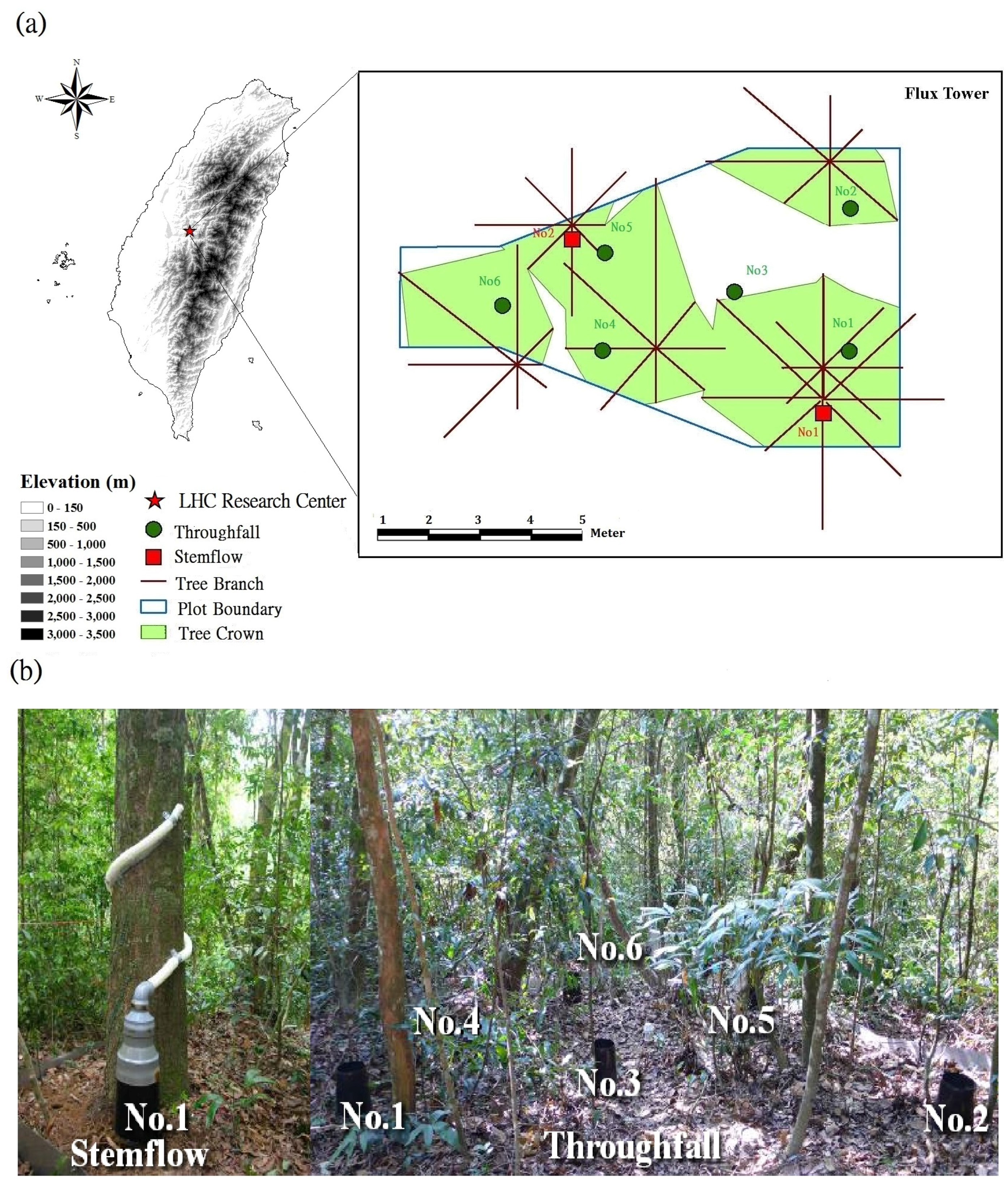
2.1. Site Description

An experiment was conducted in a Sub-watershed No. 5 at the Lien-Hua-Chih (LHC) Research Center, located in central Taiwan (${23}^{\circ }{55}^{\prime }{52}^{″}$ N, ${120}^{\circ }{53}^{\prime }{39}^{″}$ E). The elevation in that area varies from 700 m to 800 m above sea level. This study site is characterized by gently rolling terrain with a variety of tree species. The vegetation comprises a warm-to-temperate rainforest, including mixed evergreen and hardwoods. Melastomataceae, Lauraceae, Proteaceae, Rubiaceae, Araliaceae and Fagaceae are the most important tree families of the area. These distinct tree families produce a unique two layer canopy structure, which can be separated into a top-canopy and sub-canopy (diameter at breast height (DBH) is <15 cm). The average stem density and DBH for the top-canopy layer are 450 trees·ha⁻¹ and 22.8 cm, respectively. For the sub-canopy layer, the average stem density and DBH are 4645 trees·ha⁻¹ and 3.3 cm, respectively. These data were obtained from a field inventory carried out in 2013. Pteridophytes and vines are common. The dominante pteridophytes species are Athyriaceae, Blechnaceae and Cyatheaceae, and the dominante vine species are Fabaceae, Leguminoseae, Schisandraceae. The maximum LAI as measured by the LAI-2000 (LI-COR Inc., Lincoln, NE, USA) sensor is 4.91 m²·m⁻². The LAI of the epiphyte community is 0.59 m²·m⁻², was directly measured from individual samples within selected 5 meter by 5 meter plots [24]. The biomass of the tree stands and the epiphytes are 300.05 ton·ha⁻¹ and 2.76 ton·ha⁻¹, respectively [24,25].

The regional climate is warm and humid. The dry season, with less rainfall, is typically from October to April. During the wet season (May–September), precipitation is mainly brought by the typhoons originating in the Western Pacific Ocean and the South China Sea with some arising from the southwesterly summer monsoon [26]. The average annual rainfall (from 1976 to 2006) at the LHC study site is 2316.5 mm·y⁻¹, of which 71.4% occurs during the wet season [27]. For more detailed description about this study site, readers can refer to our previous study [28].

2.2. Instrumental Setup and Data Collection

An observation plot with an area of 42 m² was established adjacent to a 22 m high meteorological tower inside of the LHC Sub-catchment No. 5 for studying the interception dynamics. Throughfall was measured by six tipping bucket rain gauges (Dyacon Inc., RGTB4, Logan, UT, USA) with a measurement resolution of 0.25 mm per tip which were evenly placed throughout the plot, as suggested by Ziegler, et al. [29] (see Figure 1a). Stemflow was measured from two selected trees which accounted for 53% of the total crown projection area. Although parts of the tree crown are outside of the plot boundary, we considered this selection of trees as representative for our plot scale study. Stemflow was collected in plastic collars affixed to the tree trunks using silicon sealant (see Figure 1b). The stemflow measurements were converted into unit depth (mm) using the ratio of individual tree crown area to the open area of the rain gauge (Dyacon Inc., RGTB4, Logan, Utah USA). The scaling factors were 3.46 × 10⁻⁴ for tree No. 1 and 1.03 × 10⁻³ for tree No. 2. One tipping bucket rain gauge (Texas Electronics Inc., TR-5251, Dallas, TX, USA) was placed at the top of the flux tower for gross rainfall observation, with a measurement resolution of 0.1 mm per tip. Information on throughfall, stemflow and gross rainfall were stored by a data-logger (Campbell Scientific Inc., CR-23X, Logan, UT, USA) with a 1 minute temporal resolution in order to provide high-temporal resolution of observations. These measurements were conducted from April 2008 to April 2009. Figure 1a shows the instrumental setup at the observation plot. Individual rainfall events were identified as separated by a dry-spell of at least 6 hrs in duration. Some measurements were discarded due to instrumental errors, or errors caused by dust or leaves plugging the rain gauges. As a result, a total of 43 rainfall events were analyzed in this study (see Table 1).

Besides the aforementioned observations, temperature and humidity profiles were also made with electrical probes (Campbell Scientific Inc., HMP45C-L, Logan, UT, USA) placed at 5 m intervals from the ground surface up to a height of 20 m. Net radiation (Campbell Scientific Inc., Q-7.1, Logan, UT, USA), wind speed, wind direction (Campbell Scientific Inc., Young 05103, Logan, UT, USA) and air pressure (Campbell Scientific Inc., 092-L, Logan, UT, USA) were also measured at 20 m. A soil heat flux plate (Cambell Scientific Inc., HFT3-L REBS, Logan, UT, USA) was placed 5 cm below the surface. Meteorological data were recorded at 30 min intervals with an average of 1 min per sampling starting from the summer of 2006 to the present. These datasets were then gap-filled [30] and compiled to form a database with an hourly temporal resolution, which can be downloaded from the website. [31] LAI profile measurements were made by the LAI-2000 (LI-COR, Inc., Lincoln, NE, USA) sensor from March 2008 to April 2013. LAI values were measured along the flux tower at 5 m intervals from 5 m to 15 m above the ground. Samples were taken once a month at each level from the 4 points of the compass. For the ground level LAI measurement, the samples were taken from the top of six throughfall rain gauges at 1 m in height. In this study we used the LAI measured at ground level for the model parametrization work.

Table 1. A detailed summary of rainfall partitioning observations and parameters used in this study. A total of 43 events from May 2008 to April 2009, separated into two groups, wet season from 1 to 27 and dry season from 28 to event 43 are shown. $E^{*}$ denotes that aerodynamic resistance as measured by the eddy covariance approach; NA denotes no available data. For small rainfall events where the amount of rainfall is too small for DMC analysis, the places for canopy structural and climatic parameters are left blank.

Event	Period (min)	${\mathbf{P}}_{\mathbf{g}}$ (mm)	${\mathbf{P}}_{\mathbf{tf}}$ (mm)	${\mathbf{P}}_{\mathbf{sf}}$ (mm)	I (mm)	$\overline{\mathbf{R}}$ ($\frac{\mathbf{mm}}{\mathbf{hr}}$)	$\overline{\mathbf{E}}/\overline{\mathbf{R}}$ (%)	${\mathbf{P}}_{\mathbf{g}}^{{}^{\prime }}$ (mm)	p (%)	${\mathbf{S}}_{\mathbf{mean}}$ (mm)	${\mathbf{p}}_{\mathbf{t}}$ (%)	$\overline{\mathbf{E}}$ ($\frac{\mathbf{mm}}{\mathbf{hr}}$)	${\mathbf{E}}^{*}$ ($\frac{\mathbf{mm}}{\mathbf{hr}}$)
1	120	1.5	0.72	0.00	0.78	0.75	–	–	–	–	–	–	–
2	600	16.1	11.43	0.30	4.37	1.61	22.90	5.39	47.50	2.13	1.86	0.37	0.47
3	420	69.9	54.82	8.81	6.27	9.99	9.20	5.62	61.30	0.87	12.60	0.92	0.15
4	120	5.2	4.06	0.09	1.05	2.60	–	–	–	–	–	–	–
5	420	12.0	10.11	0.23	1.66	1.71	7.19	5.96	65.20	1.51	1.92	0.12	0.12
6	180	7.7	5.84	0.20	1.66	2.57	–	–	–	–	–	–	–
7	180	29.5	23.11	1.63	4.76	9.83	8.01	5.72	47.20	2.41	5.53	0.79	NA
8	300	19.5	14.18	1.19	4.13	3.90	16.00	3.35	41.20	1.52	6.10	0.62	0.13
9	60	0.2	0.00	0.00	0.20	0.20	–	–	–	–	–	–	–
10	60	1.7	0.63	0.00	1.07	1.70	–	–	–	–	–	–	–
11	120	0.9	0.59	0.00	0.31	0.45	–	–	–	–	–	–	–
12	480	92.4	74.78	13.22	4.40	11.55	3.70	5.40	58.40	1.19	14.31	0.43	0.20
13	240	37.3	29.97	3.38	3.95	9.33	0.20	6.79	32.20	4.33	9.06	0.02	0.23
14	240	8.7	6.43	0.09	2.18	2.18	7.98	5.10	55.50	1.79	1.03	0.83	0.18
15	360	42.1	31.37	7.01	3.72	7.02	9.30	3.47	37.70	1.49	16.65	0.64	0.10
16	120	3.3	2.12	0.02	1.16	1.65	–	–	–	–	–	–	–
17	60	0.2	0.00	0.00	0.20	0.20	–	–	–	–	–	–	–
18	240	20.1	13.72	3.13	3.25	5.03	9.48	6.24	49.20	1.55	15.57	0.48	0.21
19	240	49.1	34.16	11.43	3.51	12.28	2.90	5.07	38.20	1.97	23.28	0.36	0.16
20	60	2.1	0.97	0.02	1.71	2.70	–	–	–	–	–	–	–
21	180	44.0	30.18	11.19	2.63	14.67	1.50	5.97	31.10	2.55	25.43	0.22	0.28
22	60	2.1	0.97	0.01	1.12	2.10	–	–	–	–	–	–	–
23	360	22.6	17.06	2.79	2.75	3.77	7.00	8.72	52.40	2.46	12.35	0.26	0.16
24	60	1.3	1.06	0.00	0.24	1.30	–	–	–	–	–	–	–
25	180	14.5	13.12	0.26	1.12	4.83	1.70	3.51	68.50	0.99	1.79	0.08	0.12
26	120	4.7	3.22	0.03	1.45	2.35	–	–	–	–	–	–	–
27	300	37.4	31.16	3.58	2.66	7.48	6.60	6.26	64.80	1.20	9.57	0.49	0.08
28	120	22.0	16.02	3.20	2.78	11.00	8.00	4.04	56.60	0.93	14.55	0.88	0.16
29	480	15.8	11.64	1.90	2.26	1.98	9.19	3.17	60.50	0.60	12.03	0.18	0.12
30	240	9.5	8.24	0.22	1.04	2.38	7.31	1.67	66.40	0.41	2.32	0.17	0.11
31	60	2.1	1.23	0.00	0.87	2.10	–	–	–	–	–	–	–
32	1560	87.4	68.75	7.69	10.96	3.36	13.10	8.96	66.80	1.04	8.80	0.44	0.08
33	480	8.5	6.94	0.03	1.53	1.06	13.11	5.44	75.70	0.53	0.35	0.14	0.04
34	360	10.0	8.59	0.07	1.34	1.34	2.91	5.47	74.30	1.54	0.70	0.04	0.06
35	360	15.7	3.50	0.12	2.08	2.62	7.52	4.72	66.00	1.37	0.76	0.20	NA
36	300	7.6	5.59	0.01	2.00	1.52	23.49	4.16	68.10	0.34	0.13	0.36	NA
37	420	50.8	40.70	4.93	5.17	5.55	10.20	3.69	58.20	0.97	9.70	0.57	NA
38	60	1.4	0.63	0.00	0.77	1.40	–	–	–	–	–	–	–
39	180	3.0	1.90	0.00	1.10	1.00	–	–	–	–	–	–	–
40	120	0.6	0.28	0.00	0.32	0.30	–	–	–	–	–	–	–
41	120	4.1	3.43	0.02	0.65	2.05	–	–	–	–	–	–	–
42	720	76.0	62.11	7.31	6.58	6.33	7.50	4.02	52.7	1.22	9.54	0.48	NA
43	540	57.0	45.34	7.36	4.30	7.05	6.70	5.63	61.0	1.08	12.80	0.47	NA
Total	Wet	546.1	415.78	68.61	62.31	–	–	–	–	–	–	–	–
	Dry	371.5	294.89	32.86	43.75	–	–	–	–	–	–	–	–
% to $P_g$	Wet	100.0	76.14	12.56	11.41	Ave.	7.58	5.50	50.03	1.86	10.47	0.44	0.19
	Dry	100.0	79.69	8.85	11.78	–	9.91	4.63	64.21	0.91	6.52	0.36	0.10

Table 1. A detailed summary of rainfall partitioning observations and parameters used in this study. A total of 43 events from May 2008 to April 2009, separated into two groups, wet season from 1 to 27 and dry season from 28 to event 43 are shown. $E^{*}$ denotes that aerodynamic resistance as measured by the eddy covariance approach; NA denotes no available data. For small rainfall events where the amount of rainfall is too small for DMC analysis, the places for canopy structural and climatic parameters are left blank.

Event	Period (min)	${\mathbf{P}}_{\mathbf{g}}$ (mm)	${\mathbf{P}}_{\mathbf{tf}}$ (mm)	${\mathbf{P}}_{\mathbf{sf}}$ (mm)	I (mm)	$\overline{\mathbf{R}}$ ($\frac{\mathbf{mm}}{\mathbf{hr}}$)	$\overline{\mathbf{E}}/\overline{\mathbf{R}}$ (%)	${\mathbf{P}}_{\mathbf{g}}^{{}^{\prime }}$ (mm)	p (%)	${\mathbf{S}}_{\mathbf{mean}}$ (mm)	${\mathbf{p}}_{\mathbf{t}}$ (%)	$\overline{\mathbf{E}}$ ($\frac{\mathbf{mm}}{\mathbf{hr}}$)	${\mathbf{E}}^{*}$ ($\frac{\mathbf{mm}}{\mathbf{hr}}$)
1	120	1.5	0.72	0.00	0.78	0.75	–	–	–	–	–	–	–
2	600	16.1	11.43	0.30	4.37	1.61	22.90	5.39	47.50	2.13	1.86	0.37	0.47
3	420	69.9	54.82	8.81	6.27	9.99	9.20	5.62	61.30	0.87	12.60	0.92	0.15
4	120	5.2	4.06	0.09	1.05	2.60	–	–	–	–	–	–	–
5	420	12.0	10.11	0.23	1.66	1.71	7.19	5.96	65.20	1.51	1.92	0.12	0.12
6	180	7.7	5.84	0.20	1.66	2.57	–	–	–	–	–	–	–
7	180	29.5	23.11	1.63	4.76	9.83	8.01	5.72	47.20	2.41	5.53	0.79	NA
8	300	19.5	14.18	1.19	4.13	3.90	16.00	3.35	41.20	1.52	6.10	0.62	0.13
9	60	0.2	0.00	0.00	0.20	0.20	–	–	–	–	–	–	–
10	60	1.7	0.63	0.00	1.07	1.70	–	–	–	–	–	–	–
11	120	0.9	0.59	0.00	0.31	0.45	–	–	–	–	–	–	–
12	480	92.4	74.78	13.22	4.40	11.55	3.70	5.40	58.40	1.19	14.31	0.43	0.20
13	240	37.3	29.97	3.38	3.95	9.33	0.20	6.79	32.20	4.33	9.06	0.02	0.23
14	240	8.7	6.43	0.09	2.18	2.18	7.98	5.10	55.50	1.79	1.03	0.83	0.18
15	360	42.1	31.37	7.01	3.72	7.02	9.30	3.47	37.70	1.49	16.65	0.64	0.10
16	120	3.3	2.12	0.02	1.16	1.65	–	–	–	–	–	–	–
17	60	0.2	0.00	0.00	0.20	0.20	–	–	–	–	–	–	–
18	240	20.1	13.72	3.13	3.25	5.03	9.48	6.24	49.20	1.55	15.57	0.48	0.21
19	240	49.1	34.16	11.43	3.51	12.28	2.90	5.07	38.20	1.97	23.28	0.36	0.16
20	60	2.1	0.97	0.02	1.71	2.70	–	–	–	–	–	–	–
21	180	44.0	30.18	11.19	2.63	14.67	1.50	5.97	31.10	2.55	25.43	0.22	0.28
22	60	2.1	0.97	0.01	1.12	2.10	–	–	–	–	–	–	–
23	360	22.6	17.06	2.79	2.75	3.77	7.00	8.72	52.40	2.46	12.35	0.26	0.16
24	60	1.3	1.06	0.00	0.24	1.30	–	–	–	–	–	–	–
25	180	14.5	13.12	0.26	1.12	4.83	1.70	3.51	68.50	0.99	1.79	0.08	0.12
26	120	4.7	3.22	0.03	1.45	2.35	–	–	–	–	–	–	–
27	300	37.4	31.16	3.58	2.66	7.48	6.60	6.26	64.80	1.20	9.57	0.49	0.08
28	120	22.0	16.02	3.20	2.78	11.00	8.00	4.04	56.60	0.93	14.55	0.88	0.16
29	480	15.8	11.64	1.90	2.26	1.98	9.19	3.17	60.50	0.60	12.03	0.18	0.12
30	240	9.5	8.24	0.22	1.04	2.38	7.31	1.67	66.40	0.41	2.32	0.17	0.11
31	60	2.1	1.23	0.00	0.87	2.10	–	–	–	–	–	–	–
32	1560	87.4	68.75	7.69	10.96	3.36	13.10	8.96	66.80	1.04	8.80	0.44	0.08
33	480	8.5	6.94	0.03	1.53	1.06	13.11	5.44	75.70	0.53	0.35	0.14	0.04
34	360	10.0	8.59	0.07	1.34	1.34	2.91	5.47	74.30	1.54	0.70	0.04	0.06
35	360	15.7	3.50	0.12	2.08	2.62	7.52	4.72	66.00	1.37	0.76	0.20	NA
36	300	7.6	5.59	0.01	2.00	1.52	23.49	4.16	68.10	0.34	0.13	0.36	NA
37	420	50.8	40.70	4.93	5.17	5.55	10.20	3.69	58.20	0.97	9.70	0.57	NA
38	60	1.4	0.63	0.00	0.77	1.40	–	–	–	–	–	–	–
39	180	3.0	1.90	0.00	1.10	1.00	–	–	–	–	–	–	–
40	120	0.6	0.28	0.00	0.32	0.30	–	–	–	–	–	–	–
41	120	4.1	3.43	0.02	0.65	2.05	–	–	–	–	–	–	–
42	720	76.0	62.11	7.31	6.58	6.33	7.50	4.02	52.7	1.22	9.54	0.48	NA
43	540	57.0	45.34	7.36	4.30	7.05	6.70	5.63	61.0	1.08	12.80	0.47	NA
Total	Wet	546.1	415.78	68.61	62.31	–	–	–	–	–	–	–	–
	Dry	371.5	294.89	32.86	43.75	–	–	–	–	–	–	–	–
% to $P_g$	Wet	100.0	76.14	12.56	11.41	Ave.	7.58	5.50	50.03	1.86	10.47	0.44	0.19
	Dry	100.0	79.69	8.85	11.78	–	9.91	4.63	64.21	0.91	6.52	0.36	0.10

Figure 1. Geological location of the Lien-Hua-Chinh (LHC) Research Center and the arrangement of throughfall and stemflow collectors within observation plot (a) and the photo of the observation plot showing stemflow collector and throughfall measurements (b). The white text with black outline denotes the number of stemflow and throughfall measurements.

Figure 1. Geological location of the Lien-Hua-Chinh (LHC) Research Center and the arrangement of throughfall and stemflow collectors within observation plot (a) and the photo of the observation plot showing stemflow collector and throughfall measurements (b). The white text with black outline denotes the number of stemflow and throughfall measurements.

3. Methods

3.1. Gash Interception Model

Interception loss for a single rainfall event can be estimated by considering gross rainfall, canopy structure parameters, wet canopy evaporation rate, rainfall rate and a rainfall threshold, which is given by [23,32]

$$I=\frac{\overline{E}}{\overline{R}}{P}_g+(1-p-p_t-\frac{\overline{E}}{\overline{R}})P_g^{{}^{\prime }}$$

(1)

where $P_g$ is the amount of gross rainfall (mm); $P_g^{\prime }$ is the amount of gross rainfall necessary to saturate the canopy (mm), which can be determined by a DMC analysis [22]; p is the gap fraction or the fraction of direct throughfall (unitless); $p_t$ is the fraction of rainfall intercepted by the trunks (unitless); E is the wet canopy evaporation rate (mm·h⁻¹); R is the rainfall rate (mm·h⁻¹); and the bar denotes the average rate for a single event. The first term in Equation (1) represents the contribution of wet canopy evaporation during rainfall to the interception loss. The second term represents the contribution of wet canopy evaporation after rainfall to the interception loss or the wet canopy storage capacity ($S_{mean}$). A detailed derivation of Equation (1) is provided in Appendix A.

3.2. Wet Canopy Evaporation

Wet canopy evaporation can be directly calculated from the measured micro-meteorological variables. Neglecting the surface resistance, it is suggested that the Penman-Monteith potential evaporation equation can be applied to determine the wet canopy evaporation rate [33]. The equation is

$$E={\displaystyle \frac{\Delta (R_n-G-\frac{dQ}{dT})+(\rho c_p{\delta }_e/r_a)}{(\Delta +\gamma )}}$$

(2)

where Δ is the slope of the saturation vapor pressure to the air temperature curve (kPa·K⁻¹); γ is the psychometric constant (Pa·K⁻¹); $R_n$ is the net radiation flux (W·m⁻²); $dQ/dT$ is the storage heat flux in the forest canopy layer (J·s⁻¹· m⁻²); G is the ground heat flux (W·m⁻²); ρ is the air density (kg·m⁻³); $c_p$ is the specific heat capacity of air (kg⁻¹·K⁻¹); ${\delta }_e$ is the vapor pressure deficit (kPa); and $r_a$ is the aerodynamic resistance (s·m⁻¹).

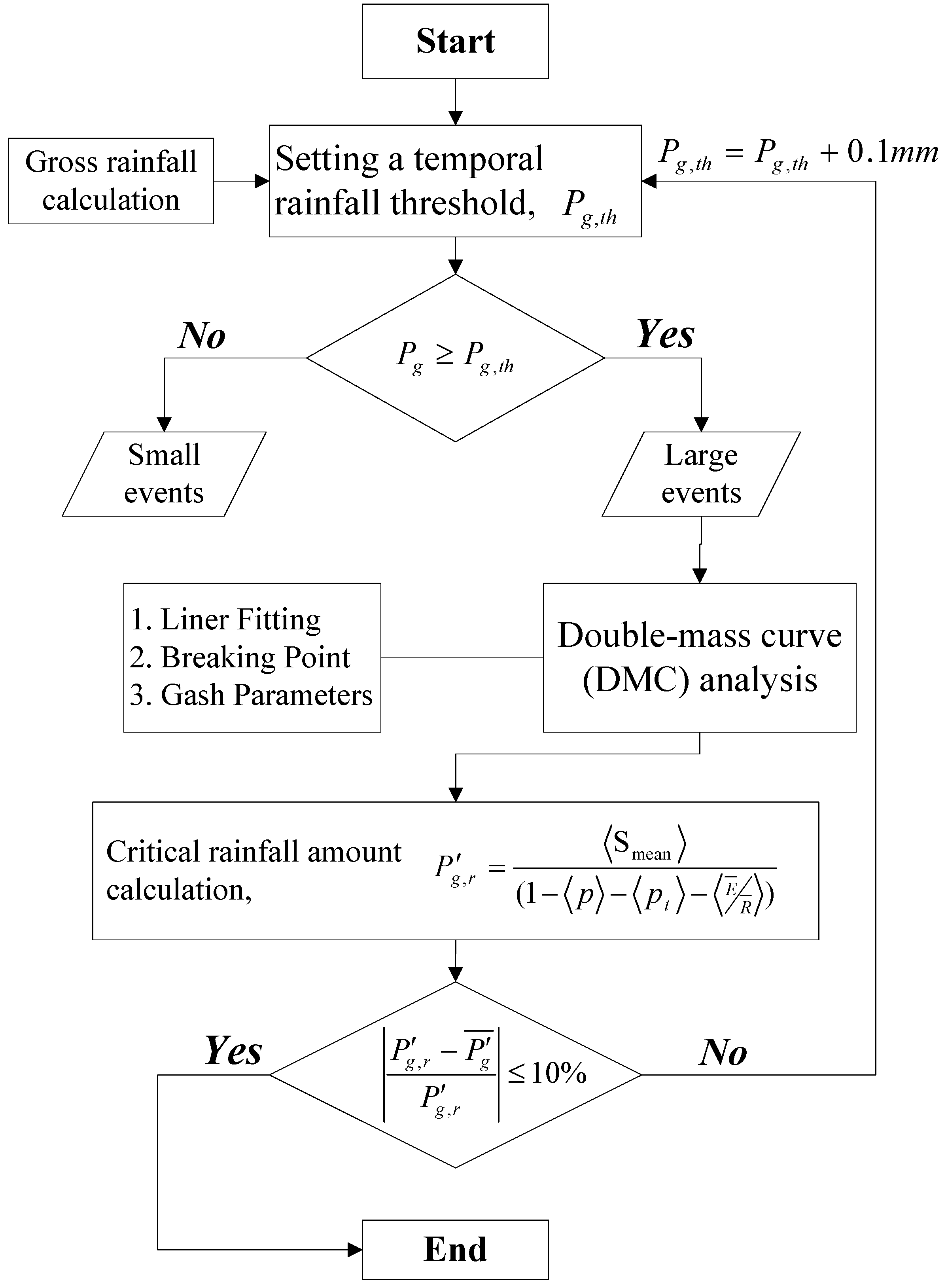
3.3. Analysis Procedure for Selecting Rainfall Events

Equation (1) can also be used to estimate the seasonal interception loss with multiple event analysis. The seasonal canopy saturation capacity can be treated as the offset of the regression line of interception loss and gross rainfall. The amount of rainfall necessary to saturate the canopy on a seasonal scale is given by the following equation:

$$P_{g,r}^{{}^{\prime }}={\displaystyle \frac{〈S_{mean}〉}{1-〈p〉-〈p_t〉-〈\frac{\overline{E}}{\overline{R}}〉}}$$

(3)

where $S_{mean}$ is the canopy water storage capacity for each rainfall event determined by DMC analysis; $P_{g,r}^{{}^{\prime }}$ is the gross rainfall necessary to saturate the canopy on a seasonal time scale; and 〈〉 is the seasonal average notation for events with a gross amount of rainfall larger than a selected threshold. The relationship between canopy saturation capacity and gap fraction can be found using Equation (1). This procedure is used to determine seasonal rainfall thresholds for both the wet and dry seasons, as the criteria for estimating parameters in the Gash model. The key point to determining $S_{mean}$ is to find a threshold value for Equation (1). Here, we propose a numerical algorithm for selecting a suitable threshold for precipitation ($P_{g,th}$) which is used to optimize these parameters for further analysis. The parameters include the uncovered fraction (p), trunk fraction ($p_t$), saturated canopy capacity ($S_{mean}$), and the fraction indicating the mean evaporation to mean rainfall rate ($\frac{\overline{E}}{\overline{R}}$ ). This procedure is described in greater detail below.

A critical rainfall amount $P_g^{{}^{\prime }}$, representing the amount of precipitation needed to saturate the canopy, is first determined by the DMC, which shows the throughfall and gross rainfall (with a 2 min time resolution) for any rainfall event larger than an initial rainfall threshold, $P_{g,th}$. After this parameters is determined, a seasonal $P_{g,r}^{{}^{\prime }}$ can be obtained from Equation (3). The arithmetic mean of the saturation rainfall needs to be consistent with the Gash model formulation for $P_{g,r}^{{}^{\prime }}$. $\overline{P_g^{{}^{\prime }}}$ is an average value for saturated gross rainfall events with a $P_g$ larger than the $P_{g,th}$ value. If the error between $\overline{P_g^{{}^{\prime }}}$ and $P_{g,r}^{{}^{\prime }}$ is in excess of 10% of the absolute error, then the initial guessed threshold (1 mm) is increased or decreased by a tiny rainfall amount (0.1 mm), prior to running the next analysis. This is repeated until the absolute error is <10%. The program will automatically stop the iteration process at this point. A computer program was written in FORTRAN code to run the above algorithm to determine the precipitation threshold for estimating the interception parameters on a seasonal time scale. Figure 2 shows the flow chart for this analysis algorithm.

Figure 2. Flow chart of the proposed algorithm for determining the rainfall threshold, $P_{g,th}$ for the DMC analysis.

Figure 2. Flow chart of the proposed algorithm for determining the rainfall threshold, $P_{g,th}$ for the DMC analysis.

4. Results

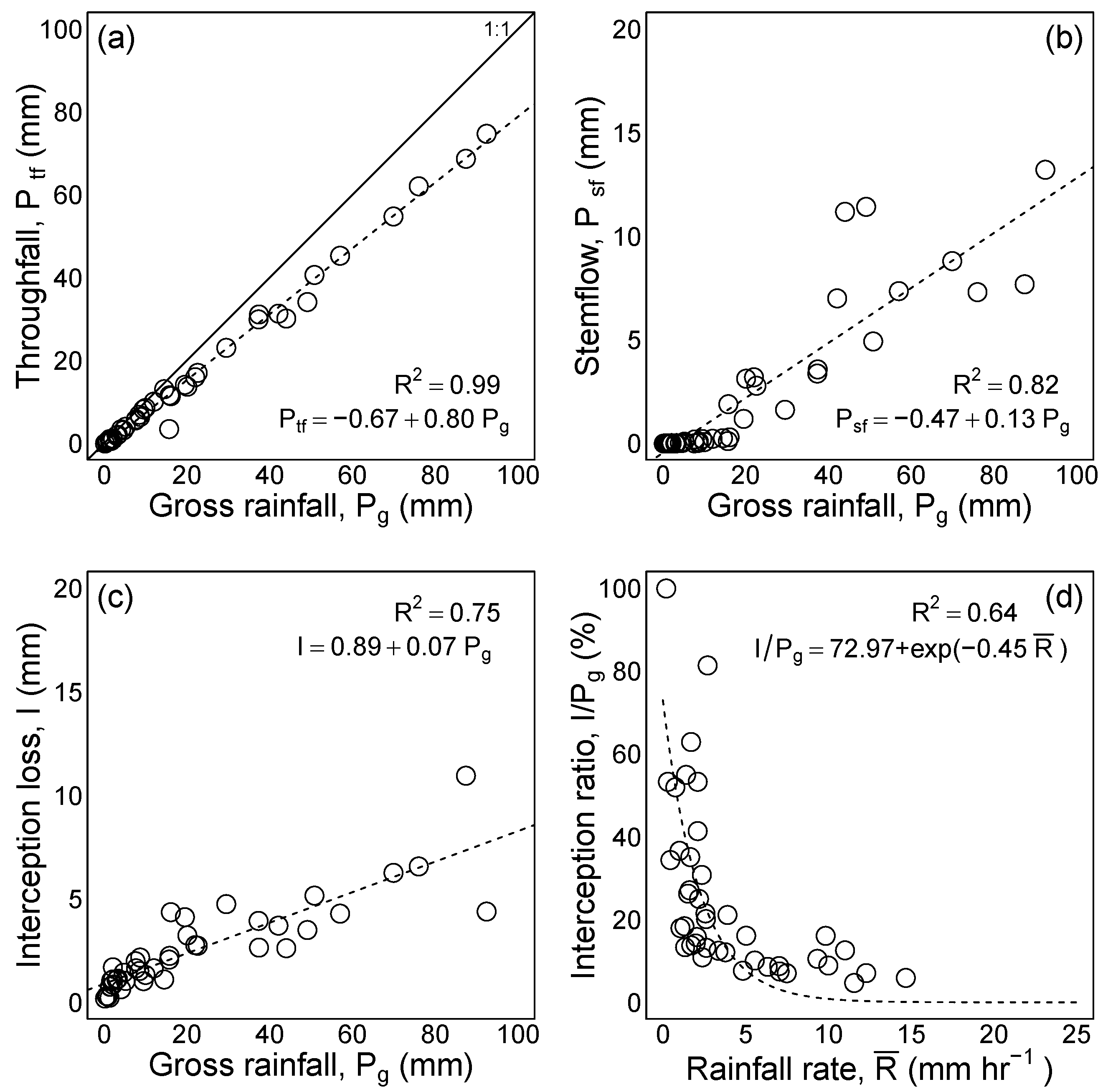
4.1. Canopy Water Balance and Interception

Table 1 summarizes the observation results for canopy water balance for each rainfall event throughout the study period. Measured rainfall accumulations for the wet and the dry seasons were 546.1 mm and 371.5 mm, respectively. The amount of rainfall ranged from 0.2 mm to 92.4 mm. Cumulative throughfall for the wet and the dry seasons was 415.8 mm and 294.9 mm, representing 76.1% and 79.4% of the seasonal rainfall, respectively. Cumulative stemflow for the wet season was estimated to be 86.6 mm, representing 12.5% of the wet season rainfall, while the dry season estimate only accounted for 8.8% of the dry season rainfall (32.8 mm). The percentage of seasonal cumulative rainfall interception loss was similar (approximately 12%): 62.3 mm for the wet season and 43.8 mm for the dry season.

The relationships between gross rainfall and throughfall, stemflow and interception loss are presented in Figure 3a–c and the relationship between rainfall interception ratio and rainfall intensity is shown in Figure 3d. The results show that better performance was obtained using a simple linear regression approach to partition the gross rainfall to throughfall than was the case for stemflow or interception loss. The throughfall, stemflow and interception loss can be expressed as functions of gross rainfall, as follows: $P_{tf}=-0.67+0.80P_g$ ($R^2=0.99$), $P_{sf}=-0.47+0.13P_g$ ($R^2=0.82$) and $I=0.89+0.07P_g$ ($R^2=0.75$). The rainfall interception ratio is also parametrized as a function of rainfall intensity, i.e., $I/P_g=72.97+exp(-0.45\overline{R})$ ($R^2=0.64$).

Figure 3. Scatter plots of gross rainfall $P_g$ against throughfall $P_{tf}$ (a), stemflow $P_{sf}$ (b), interception loss I (c) and the relationship between the rainfall interception ratio and rainfall rate $\overline{R}$ (d). The dashed lines indicate the regression equations of $P_{tf}=-0.67+0.80P_g$, $P_{sf}=-0.47+0.13P_g$, $I=0.89+0.07P_g$ and $I/P_g=72.97+exp(-0.45\overline{R})$.

Figure 3. Scatter plots of gross rainfall $P_g$ against throughfall $P_{tf}$ (a), stemflow $P_{sf}$ (b), interception loss I (c) and the relationship between the rainfall interception ratio and rainfall rate $\overline{R}$ (d). The dashed lines indicate the regression equations of $P_{tf}=-0.67+0.80P_g$, $P_{sf}=-0.47+0.13P_g$, $I=0.89+0.07P_g$ and $I/P_g=72.97+exp(-0.45\overline{R})$.

4.2. Wet Canopy Evaporation

The $\overline{E}$ values are derived both from DMC analysis and the Penman-Monteith equation (using the aerodynamic resistance directly measured by a sonic anemometer [34]). By making use of DMC analysis, $\overline{E}$ can be determined for larger rainfall events under the condition of $P_g>P_g^{{}^{\prime }}$, for both the dry and wet seasons. The seasonal average of $\overline{E}$ is estimated to be 0.44 mm·h⁻¹ for the wet season, while the seasonal average of $\overline{E}$ is calculated to be 0.36 mm·h⁻¹ for the dry season.

The Penman-Monteith equation (Equation (2)), with the aerodynamic resistance retrieved from the eddy covariance direct measurement, is also applied for the calculation of $\overline{E}$. The results are presented in the last column of Table 1 ($E^{*}$). The seasonal average of $E^{*}$ is 0.19 mm·h⁻¹ for the wet season and 0.10 mm·h⁻¹ for the dry season.

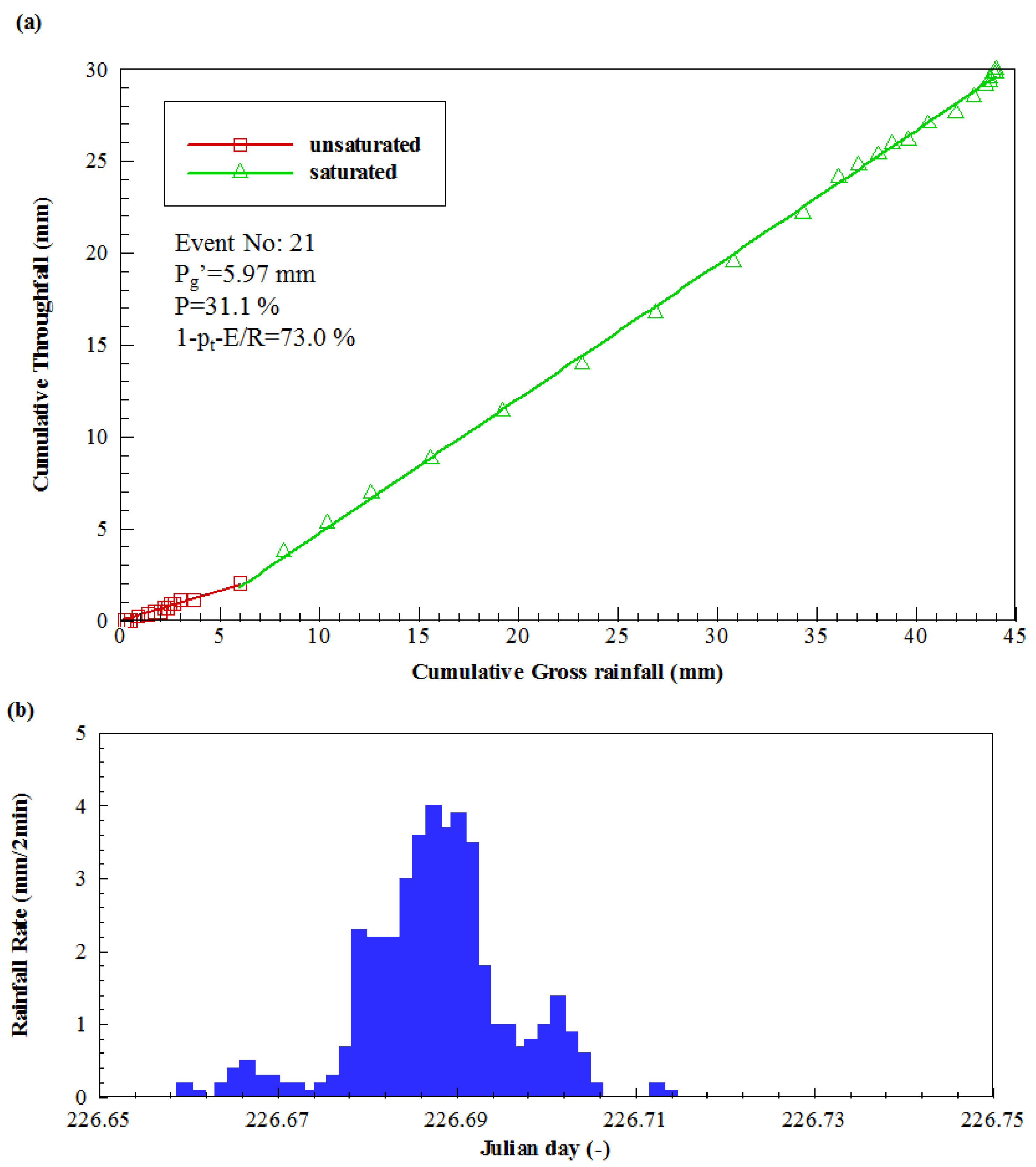
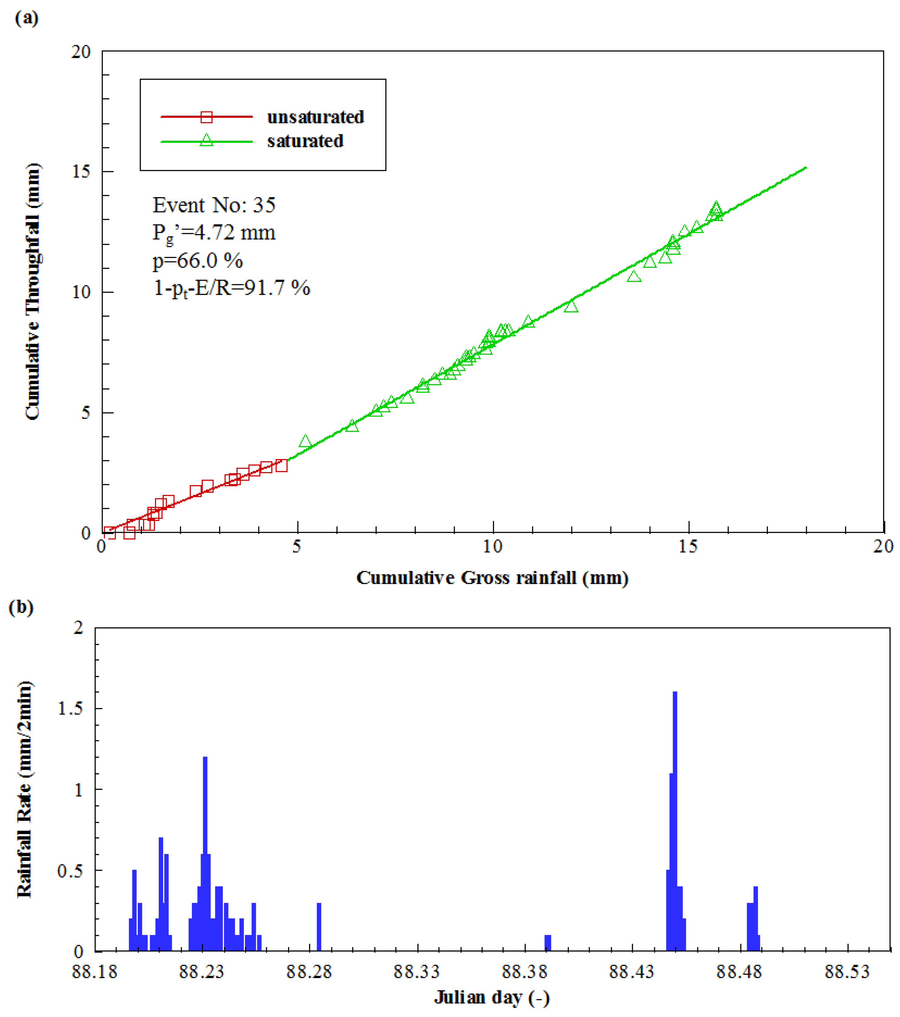
4.3. Single Event Analysis

Figure 4 presents the DMC (i.e., accumulated gross rainfall in relation to the accumulated throughfall) and the rainfall histogram for event 21 during the wet season. This event began at 16:00 on the 226th Julian-day 2008 and lasted for 3 h. During this period, 44.0 mm of rain fell ($P_g$ = 44.0 mm). This event was characterized by high rainfall intensity ($\overline{R}$ = 14.67 mm·h⁻¹), continuous rainfall, but with small rain drops at the beginning (see Figure 4b). I was 2.63 mm, its principal source being from the water stored in the canopy, which gradually evaporated after the rain ceased. In this case, $S_{mean}$ was 2.55 mm and $P_g^{{}^{\prime }}$ was 5.97 mm. The gap fraction (p) was quite small, only 31.10%. $\overline{E}/\overline{R}$ was 1.50%, with $\overline{E}$ estimated at a rate of 0.22 mm·h⁻¹. Most of the I was contributed from the $S_{mean}$.

Figure 4. Plots of the DMC (a) and rainfall histogram (b) for event 21 during the wet season.

Figure 4. Plots of the DMC (a) and rainfall histogram (b) for event 21 during the wet season.

The DMC and the rainfall histogram of event 35 are shown in Figure 5. This event started at mid-night of the 88th Julian-day 2009 and lasted 6 h. This event was characterized by weak rainfall intensity ($\overline{R}$ = 2.62 mm·h⁻¹), long duration, and intermittent rainfall with an accumulation of 15.7 mm ($P_g$) during the dry season (see Figure 5b). The $S_{mean}$ was 1.37 mm and $P_g^{{}^{\prime }}$ was 4.72 mm. In comparison with event 21, the gap fraction (p) increased from 31.1% to 66.0%. However, the difference in I was small and I was estimated to be 2.08 mm. Note, almost 50% of I was contributed from $\overline{E}$ (0.20 mm·h⁻¹) during the period of rainfall, the remaining 50% being attributable to the $S_{mean}$.

Figure 5. Plots of DMC (a) and rainfall histogram (b) for event 35 during the dry season.

Figure 5. Plots of DMC (a) and rainfall histogram (b) for event 35 during the dry season.

The climatic and canopy structural parameters of these two events are quite different with large $P_g^{{}^{\prime }}$ found for event 21 (5.97 mm), while the $P_g^{{}^{\prime }}$ for event 35 is only 4.72 mm. The variation in $\overline{E}$ is small in comparison with the variation in $\overline{R}$; in addition, the observed variation in $S_{mean}$ shows a decrease from 2.55 mm to 1.37 mm.

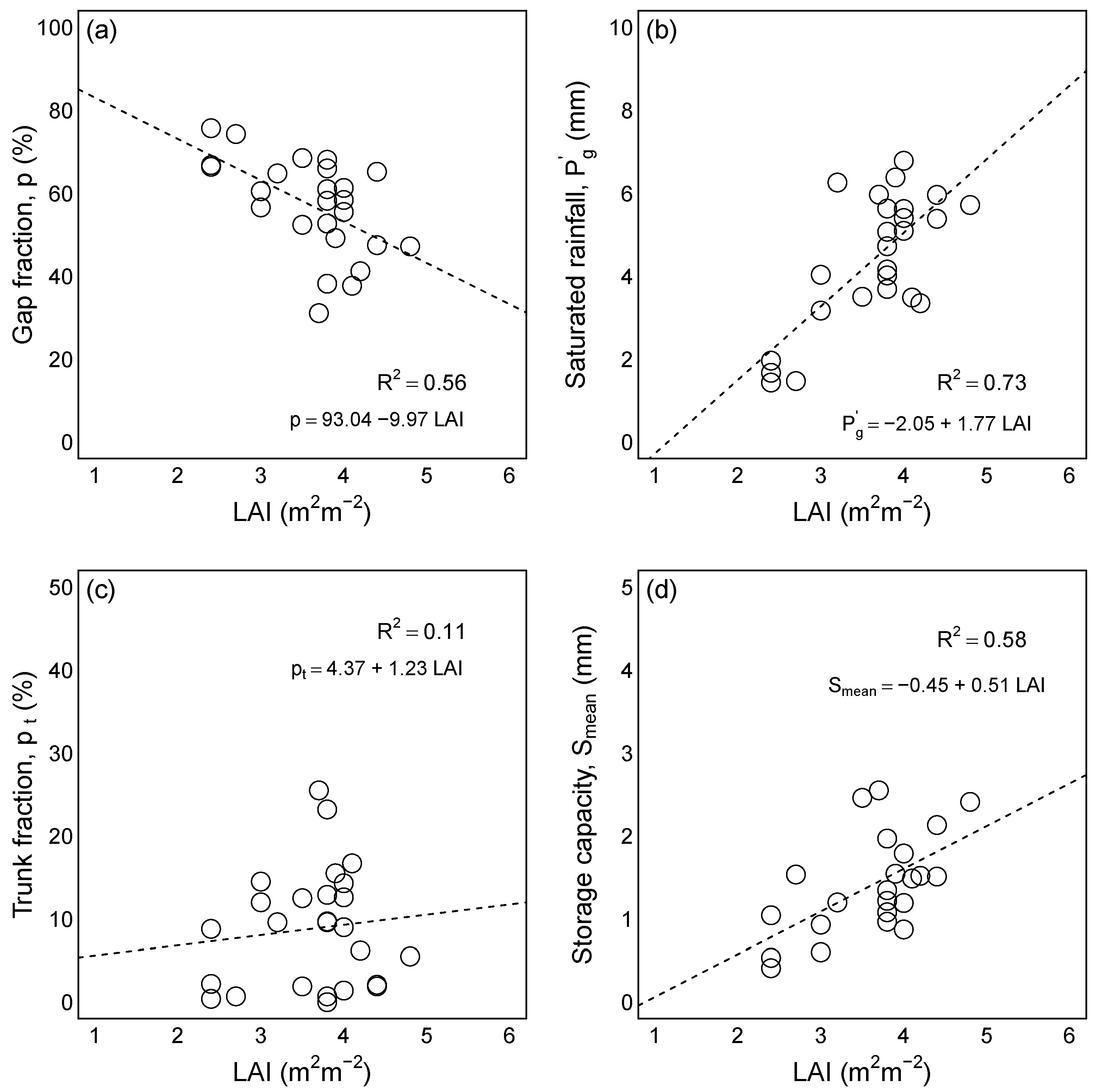
4.4. Multiple Event Analysis and Model Parametrisation

Following the analysis procedure, the seasonal $P_{g,th}$ was retrieved to classify rainfall events as either small or large during different seasons. $P_{g,th}$ is found to be 7.80 mm for the wet season and 4.70 mm for the dry season (see Table 1). The seasonal saturated rainfall ($P_{g,r}^{{}^{\prime }}$) is 5.51 mm for the wet season. This value is comparatively larger than that found in the dry season (4.64 mm). The difference between these two values can be attributed to the combined results of changes in the canopy structure and wet canopy evaporation rate before the canopy becomes saturated. Temporal variability of the canopy water storage capacity is observed, associated with changes in the LAI (see Table 1). The $S_{mean}$ ranged from 0.34 mm to 1.54 mm for the dry season and from 0.90 mm to 4.33 mm for the wet season. The maximum $S_{mean}$ value was 4.33 mm in July gradually decreasing to a smaller value during the dormant season.

Large rainfall events, where the gross rainfall is less than the seasonal saturated rainfall, can be utilized for model parametrization with monthly LAI observation data. Figure 6 shows scatter plots of the leaf area index LAI against gap fraction (p), saturated gross precipitation ($P_g^{{}^{\prime }}$), trunk cover fraction ($p_t$) and mean storage canopy capacity ($S_{mean}$). Here, a simple linear relationship is applied to show the linked relationship between the aforementioned parameters and the LAI. The results of regressions are also given in Figure 6. The gap fraction, saturated rainfall, trunk fraction and storage capacity can be expressed as the function of LAI, in terms of the following equations: $p=93.04-9.97LAI$, $P_g^{{}^{\prime }}=-2.05+1.77LAI$, $p_t=4.37+1.23LAI$ and $S_{mean}=-0.45+0.51LAI$. The correlation coefficients for each parameter are over 0.56, except for the relationship between the trunk fraction ($p_t$) and LAI, which presents a poor correlation with an $R^2$ value of 0.11.

Figure 6. Scatter plots of LAI against gap fraction p (a); saturated gross precipitation $P_g^{{}^{\prime }}$ (b); trunk cover fraction $p_t$ (c) and mean storage canopy capacity $S_{mean}$ (d). The dashed lines indicate the regression equations of $p=93.04-9.97LAI$, $P_g^{{}^{\prime }}=-2.05+1.77LAI$, $p_t=4.37+1.23LAI$ and $S_{mean}=-0.45+0.51LAI.$

Figure 6. Scatter plots of LAI against gap fraction p (a); saturated gross precipitation $P_g^{{}^{\prime }}$ (b); trunk cover fraction $p_t$ (c) and mean storage canopy capacity $S_{mean}$ (d). The dashed lines indicate the regression equations of $p=93.04-9.97LAI$, $P_g^{{}^{\prime }}=-2.05+1.77LAI$, $p_t=4.37+1.23LAI$ and $S_{mean}=-0.45+0.51LAI.$

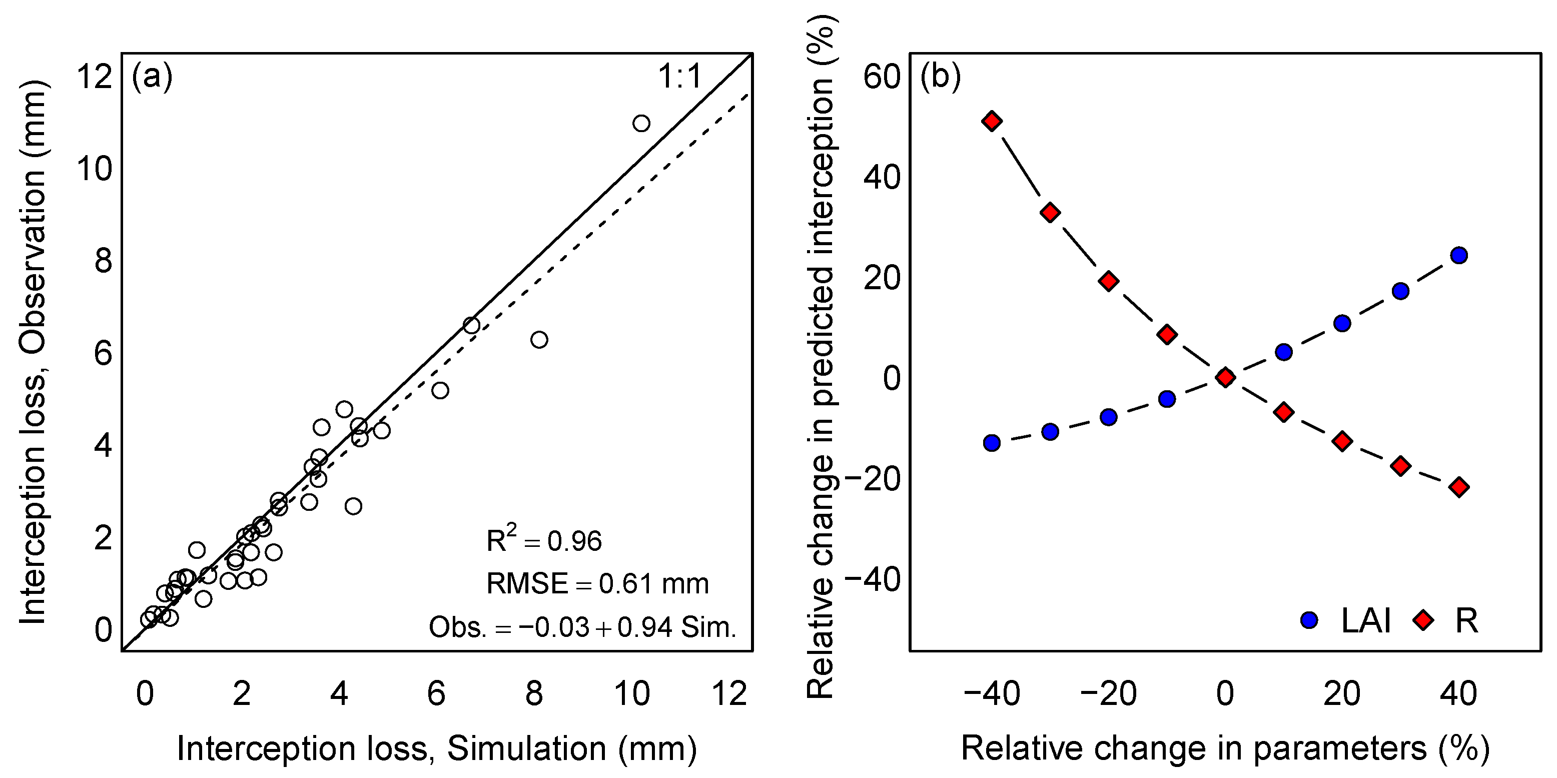
4.5. Model Error Assessment and Sensitivity Analysis

The performance obtained using the Gash interception model with the proposed LAI parametrization approach is examined with the dataset covering both wet and dry seasons from April 2008 to April 2009. Figure 7a presents the scatter plot of the model simulations against the observations. The model shows a good performance with an R² of 0.96 and an RMSE (root mean square error) of 0.61 mm.

Figure 7. Model error assessment and sensitivity analysis. (a) scatter plots of interception loss observation against simulation results; (b) the model sensitivity to the canopy parameter (LAI) and climatic parameter ($\overline{R}$).

Figure 7. Model error assessment and sensitivity analysis. (a) scatter plots of interception loss observation against simulation results; (b) the model sensitivity to the canopy parameter (LAI) and climatic parameter ($\overline{R}$).

The results of sensitivity analysis of the canopy parameter LAI and the climatic parameters used in this model are presented in Figure 7b. A set of initial values, LAI = 3.0 m·m⁻², $\overline{R}$ = 4.0 mm·h⁻¹ and $\overline{E}$ = 0.4 mm·h ⁻¹, are applied for the reference interception loss calculation using the Equation (1). The results show that the model is highly sensitive to rainfall rate $\overline{R}$: a decrease of 40% in $\overline{R}$ increases interception loss by 50.9% and an increase of 40% in $\overline{R}$ reduces interception loss by 28.1%. In comparison, the model is moderately sensitive to LAI . An increase of 40% in LAI produces a 24.2% increase in interception loss and a decrease of 40% in LAI also results in a decrease of 13.1% in interception loss.

5. Discussion

5.1. Canopy Structure Parameters

In this study, several linear relationships have been built up to describe the dynamics of canopy structure parameters, i.e., $S_{mean}$, $P_g^{{}^{\prime }}$, p and $p_t$, based on the measured monthly LAI values (see Figure 6). These relationships are also applied for the Gash interception model for I estimation, resulting in an average model error of 0.61 mm on interception loss estimation.

The seasonal $S_{mean}$, as associated with the canopy development, is estimated to be 1.86 mm for the wet season and 0.91 mm for the dry, respectively. The absolute values are similar to the findings obtained in previous studies [1,7,13], which reported a canopy water storage capacity ranging from 0.97 mm to 4.30 mm for the subtropical mixed forests. According to a former biomass inventory, the maximum LAI of pteridophyte accounts for nearly 10% of the total LAI, although there may be seasonal variation in the pteridophyte and vine species. If we apply this value to our parameterization results, we find that the epiphyte community could contribute nearly 0.30 mm (0.51 × 0.59) to the total storage capacity (1.98 mm for the wet season). Comparison of the values with these obtained from other studies [35,36] shows that this value is still acceptable but approaches the lower bound in the 0.20–3.00 mm range for the epiphyte community, as reported by Van Stan and Pypker [37].

5.2. Throughfall and Stemflow Yield

Based on our multi-events analysis (see Figure 6), we observe a negative correlation between canopy coverage (LAI) and throughfall. Both the dense crown cover and new branch development during the wet/growing season can reduced the throughfall yield. However, the effect of canopy coverage on rainfall stemflow ratio ($P_g/P_{sf}$) is complicated. A very weak positive correlation between canopy coverage (LAI) and steamflow (trunk fraction) is found. A possible explanation for this weak positive correlation could be the representation of the stemflow measurement for the two layer canopy structure, or inadequate parametrization. Although we did not directly measure the sub-canopy stemflow yield, in the furture we propose measuring the sub-canopy stemflow to address this issue. If we assume that the difference between the top-canopy and sub-canopy stemflow yield is small, this effect might be due to the interaction between the local climate (such as seasonal rainfall intensity) and canopy structure (such as wether it is comprised of an epiphyte community or layered canopy). For example, some studies [38,39,40] have reported that stemflow might have a larger value under low rainfall intensity conditions than under strong rainfall conditions, although our results still present a relatively small stemflow during the dry season with a low rainfall intensity and a low canopy coverage.

The positive relationship between stemflow yield and crown cover has often been assumed for stemflow modeling in forest hydrology, such as in the past studies carried out by Aboal, et al. and Park, et al. [9,41]. However, recent studies and reviews [36,40,42] have indicated that the stemflow yield is a more complex phenomenon dependent on tree bark properties, branch angle and lichen cover, resulting in a negative correlation between stemflow yield and crown cover fraction. A more sophisticated stemflow measurement is required to understand the mechanism of stemflow yield at this study site.

5.3. Wet Canopy Evaporation Rate

Seasonal averages of $\overline{E}$ are retrieved using DMC analysis and Penman-Monteith approach. The seasonal averages of $\overline{E}$ for both dry and wet seasons are nearly 0.40 mm·h⁻¹. These rates are similar to those reviewed by Deguchi, et al. [7], within the range from 0.13 mm to 0.60 mm·h⁻¹ for the subtropical climate region. However, there is a gap, of nearly 0.2 mm·h⁻¹, between $\overline{E}$ and $E^{*}$. This discrepancy might be due to the assumptions/limitations of the eddy covariance method, which failed to obtain the contribution of vertical advection flux during the observation periods. This is also consistent with the findings of recent studies made by Staelens, et al. [43] and Saito, et al. [44]. It is suggested that the advection process makes a considerable contribution to the $\overline{E}$ at our study site.

5.4. Rainfall Interception Loss

The amount of I for annual precipitation may range over 10%–30% for various plant communities and climate regions [22,45]. The annual I for a mixed hardwood forest is found to be 10.0% of the annual rainfall in Taiwan [14]. Changes in types of vegetation, such as the conversion of natural forests to betel nut plantations, have reduced the amount of annual I from 11.0% of annual rainfall to 8.3% [46]. In this study, the annual I accounts for nearly 12% of annual rainfall. The seasonal differences in I are small, despite distinguishable changes in the canopy structure and climatological state, which is consistent with the finding of Deguchi, et al. [7].

The I can be separated into two components, $\overline{E}$ during rainfall and $\overline{E}$ after rainfall [1]. We further applied Equation (1) to investigate the temporal variation of these two components of seasonal I. The analysis results show that these two components to seasonal I are quite different in amount (see Figure 8). During the wet season, the $\overline{E}$ after rainfall accounts for nearly 40% of the wet season I; however, this ratio descends to nearly 17% during the dry season, while $S_{mean}$ in dry seasonal is only half of the wet season $S_{mean}$. The variation of seasonal $S_{mean}$ seems to show a linear relationship to the proportion of $\overline{E}$ after rainfall to the seasonal I.

The variation in the canopy structure and rainfall rate only change the amount of interception components, resulting in a similar $I/P_g$ ratio for both seasons. However, this unique $I/P_g$ ratio might just be a coincidence, if there are more and more small rainfall events ($P_g<P_g^{{}^{\prime }}$) whether in the wet season or the dry season. For this instance, the $S_{mean}$ will dominate the rainfall interception process due to the change in the local rainfall features.

Figure 8. Partitioning of interception loss according to Equation (1) during the wet season (a), the dry season (b). The red portion represents wet canopy evaporation during rainfall and the blue portion represents wet canopy evaporation after rainfall has ceased.

Figure 8. Partitioning of interception loss according to Equation (1) during the wet season (a), the dry season (b). The red portion represents wet canopy evaporation during rainfall and the blue portion represents wet canopy evaporation after rainfall has ceased.

6. Conclusions

The amount of I associated with seasonal changes in the canopy structure, rainfall features and micro-meteorological conditions is derived from direct observations of $P_g$, $P_{tf}$ and $P_{sf}$ from April 2008 to April 2009, as well as simulated using the Gash interception model. The dry and wet seasonal interception losses are found to be similar, amounting to 12% of the seasonal precipitation, but the interception components vary depending on changes in the canopy structure, rainfall intensity and micro-meteorological conditions.

For the wet season, 41.8% of the seasonal I is contributed by $\overline{E}$ after rainfall, due to a large $S_{mean}$ (1.86 mm). For the dry season, the contribution of $\overline{E}$ after rainfall to the dry season I is reduced from 41.8 % to 17.1% in relation to case with a small $S_{mean}$ (0.91 mm) and a reduced LAI, while the $\overline{E}$ during rainfall contributes most of the dry season I. Reduction of the covered fraction in the dry season has noticeable effects on the seasonal stemflow and throughfall. In consequence, the effect of canopy structural and climatic changes on the water balance reflects a trade-off between $P_{sf}/P_g$ and $P_{tf}/P_g$ on the seasonal time scale.

References

1. Link, T.E.; Unsworth, M.; Marks, D. The dynamics of rainfall interception by a seasonal temperate rainforest. Agric. For. Meteorol. 2004, 124, 171–191. [Google Scholar] [CrossRef]
2. Pypker, T.G.; Bond, B.J.; Link, T.E.; Marks, D.; Unsworth, M.H. The importance of canopy structure in controlling the interception loss of rainfall: Examples from a young and an old-growth Douglas-fir forest. Agric. For. Meteorol. 2005, 130, 113–129. [Google Scholar] [CrossRef]
3. Muzylo, A.; Llorens, P.; Valente, F.; Keizer, J.; Domingo, F.; Gash, J. A review of rainfall interception modelling. J. Hydrol. 2009, 370, 191–206. [Google Scholar] [CrossRef]
4. Domingo, F.; Sánchez, G.; Moro, M.J.; Brenner, A.J.; Puigdefábregas, J. Measurement and modelling of rainfall interception by three semi-arid canopies. Agric. For. Meteorol. 1998, 91, 275–292. [Google Scholar] [CrossRef]
5. Toba, T.; Ohta, T. An observational study of the factors that influence interception loss in boreal and temperate forests. J. Hydrol. 2005, 313, 208–220. [Google Scholar] [CrossRef]
6. Zhang, Y.F.; Wang, X.P.; Hu, R.; Pan, Y.X.; Paradeloc, M. Rainfall partitioning into throughfall, stemflow and interception loss by two xerophytic shrubs within a rain-fed re-vegetated desert ecosystem, northwestern China. J. Hydrol. 2015, 527, 1084–1095. [Google Scholar] [CrossRef]
7. Deguchi, A.; Hattori, S.; Park, H.T. The influence of seasonal changes in canopy structure on interception loss: Application of the revised Gash model. J. Hydrol. 2006, 318, 80–102. [Google Scholar] [CrossRef]
8. Klaassen, W.; Bosveld, F.; de Water, E. Water storage and evaporation as constituents of rainfall interception. J. Hydrol. 1998, 212–213, 36–50. [Google Scholar] [CrossRef]
9. Aboal, J.R.; Morales, D.; Hernández, M.; Jiménez, M.S. The measurement and modelling of the variation of stemflow in a laurel forest in Tenerife, Canary Islands. J. Hydrol. 1999, 221, 161–175. [Google Scholar] [CrossRef]
10. Fleischbein, K.; Wilcke, W.; Goller, R.; Boy, J.; Valarezo, C.; Zech, W.; Knoblich, K. Rainfall interception in a lower montane forest in Ecuador: Effects of canopy properties. Hydrol. Process. 2005, 19, 1355–1371. [Google Scholar] [CrossRef]
11. Loustau, D.; Berbigier, P.; Granier, A. Interception loss, throughfall and stemflow in a maritime pine stand. II. An application of Gash’s analytical model of interception. J. Hydrol. 1992, 138, 469–485. [Google Scholar] [CrossRef]
12. Iida, S.; Tanaka, T.; Sugita, M. Change of evapotranspiration components due to the succession from Japanese red pine to evergreen oak. J. Hydrol. 2006, 326, 166–180. [Google Scholar] [CrossRef]
13. Herbst, M.; Rosier, P.T.W.; McNeil, D.D.; Harding, R.J.; Gowing, D.J. Seasonal variability of interception evaporation from the canopy of a mixed deciduous forest. Agric. For. Meteorol. 2008, 148, 1655–1667. [Google Scholar] [CrossRef]
14. Lu, S.; Tang, K. Study on Rainfall Interception Characteristics of Natural Hardwood Forest in Central Taiwan; Bulletin of Taiwan Forestry Research Institute; Taiwan Forestry Research Institute: Taipei, Taiwan, 1995; Volume 10, pp. 447–457. [Google Scholar]
15. Lin, T.C.; Hsia, Y.J.; King, H. A study on rainfall interception of a natural hardwood forest in northeastern Taiwan. Taiwan J. For. Sci. 1996, 11, 393–400. [Google Scholar]
16. Lu, S.Y.; Cheng, J.D.; Brooks, K.N. Managing forests for watershed protection in Taiwan. For. Ecol. Manag. 2001, 143, 77–85. [Google Scholar] [CrossRef]
17. Chiang, P.N.; Zhuang, S.Y.; Wang, Y.N.; Wang, W.; Wang, M.K.; Lin, S.T. Soil Organic Matter and Soil Physicochemical Properties Associated with Forest Fires in Central Taiwan. Soil Sci. 2008, 173, 768–778. [Google Scholar] [CrossRef]
18. Lin, T.C.; Hamburg, S.P.; Lin, K.C.; Wang, L.J.; Chang, C.T.; Hsia, Y.J.; Vadeboncoeur, M.A.; Mabry McMullen, C.M.; Liu, C.P. Typhoon Disturbance and Forest Dynamics: Lessons from a Northwest Pacific Subtropical Forest. Ecosystems 2011, 14, 127–143. [Google Scholar] [CrossRef]
19. Lugo, A.E. Visible and invisible effects of hurricanes on forest ecosystems: An international review. Austral Ecol. 2008, 33, 368–398. [Google Scholar] [CrossRef]
20. Lin, K.C.; Hamburg, S.P.; Tang, S.L.; Hsia, Y.J.; Lin, T.C. Typhoon effects on litterfall in a subtropical forest. Can. J. For. Res. 2003, 33, 2184–2192. [Google Scholar] [CrossRef]
21. Chi, C.H.; McEwan, R.W.; Chang, C.T.; Zheng, C.; Yang, Z.; Chiang, J.M.; Lin, T.C. Typhoon Disturbance Mediates Elevational Patterns of Forest Structure, but not Species Diversity, in Humid Monsoon Asia. Ecosystems 2015, 18, 1410–1423. [Google Scholar] [CrossRef]
22. Dingman, S. Physical Hydrology, 2nd ed.; Prentice Hall: Upper Saddle River, NJ, USA, 2002. [Google Scholar]
23. Gash, J.H.C. An analytical model of rainfall interception by forests. Q. J. R. Meteorol. Soc. 1979, 105, 43–55. [Google Scholar] [CrossRef]
24. Horng, F.W.; Hsia, Y.J.; Tang, K.J. An Estimation of Aboveground Biomass and Leaf Area in a Secondary Warm Temperate Montane Rain Forest at Lien-Hua-Chi Area; Taiwan Forestry Research Institute: Taipei, Taiwan, 1986. [Google Scholar]
25. McEwan, R.W.; Lin, Y.C.; Sun, I.F.; Hsieh, C.F.; Su, S.H.; Chang, L.W.; Song, G.Z.M.; Wang, H.H.; Hwong, J.L.; Lin, K.C.; et al. Topographic and biotic regulation of aboveground carbon storage in subtropical broad-leaved forests of Taiwan. For. Ecol. Manag. 2011, 262, 1817–1825. [Google Scholar] [CrossRef]
26. Chen, C.S.; Chen, Y.L. The Rainfall Characteristics of Taiwan. Mon. Weather Rev. 2003, 131, 1323–1341. [Google Scholar] [CrossRef]
27. Hwong, J.L. Studies on the Characteristics of Hydrology and Water Chemistry between Natural Hardwood and China-Fir Plantation Forests in Lienhuachih Experimental Watersheds. Ph.D. Thesis, National Taiwan University, Taipei, Taiwan, 2010. [Google Scholar]
28. Chen, Y.Y.; Chu, C.R.; Li, M.H. A gap-filling model for eddy covariance latent heat flux: Estimating evapotranspiration of a subtropical seasonal evergreen broad-leaved forest as an example. J. Hydrol. 2012, 468–469, 101–110. [Google Scholar] [CrossRef]
29. Ziegler, A.D.; Giambelluca, T.W.; Nullet, M.A.; Sutherland, R.A.; Tantasarin, C.; Vogler, J.B.; Negishi, J.N. Throughfall in an evergreen-dominated forest stand in northern Thailand: Comparison of mobile and stationary methods. Agric. For. Meteorol. 2009, 149, 373–384. [Google Scholar] [CrossRef]
30. Chen, Y.Y.; Li, M.H. Determining adequate averaging periods and reference coordinates for eddy covariance measurements of surface heat and water vapor fluxes over mountainous terrain. Terr. Atmos. Ocean. Sci. 2012, 23, 685–701. [Google Scholar] [CrossRef]
31. Surface Hydrology Lab., National Central University. Available online: http://hydro.ihs.ncu.edu.tw/data.html (accessed on 22 December 2015).
32. Gash, J.H.C.; Valente, F.; David, J.S. Estimates and measurements of evaporation from wet, sparse pine forest in Portugal. Agric. For. Meteorol. 1999, 94, 149–158. [Google Scholar] [CrossRef]
33. Rutter, J.; Kershaw, K.; Robins, P.; Morton, A. A predictive model of rainfall interception in forests, 1. Derivation of the model from observations in a plantation of Corsican pine. Agric. Meteorol. 1971, 9, 367–384. [Google Scholar] [CrossRef]
34. Van Der Tol, C.; Gash, J.H.C.; Grant, S.J.; McNeil, D.D.; Robinson, M. Average wet canopy evaporation for a Sitka spruce forest derived using the eddy correlation-energy balance technique. J. Hydrol. 2003, 276, 12–19. [Google Scholar] [CrossRef]
35. Levia, D.F.; Frost, E.E. Variability of throughfall volume and solute inputs in wooded ecosystems. Prog. Phys. Geogr. 2006, 30, 605–632. [Google Scholar] [CrossRef]
36. Levia, D.F.; Germer, S. A review of stemflow generation dynamics and stemflow-environment interactions in forests and shrublands. Rev. Geophys. 2015. [Google Scholar] [CrossRef]
37. Van Stan, J.T.; Pypker, T.G. A review and evaluation of forest canopy epiphyte roles in the partitioning and chemical alteration of precipitation. Sci. Total Environ. 2015, 536, 813–824. [Google Scholar] [CrossRef] [PubMed]
38. Mauchamp, A.; Janeau, J. Water funnelling by the crown of Flourensia cernua, a Chihuahuan Desert shrub. J. Arid Environ. 1993, 25, 299–306. [Google Scholar] [CrossRef]
39. Crockford, R.H.; Richardson, D.P. Partitioning of rainfall into throughfall, stemflow and interception: Effect of forest type, ground cover and climate. Hydrol. Process. 2000, 14, 2903–2920. [Google Scholar] [CrossRef]
40. Levia, D.F.; Frost, E.E. A review and evaluation of stemflow literature in the hydrologic and biogeochemical cycles of forested and agricultural ecosystems. J. Hydrol. 2003, 274, 1–29. [Google Scholar] [CrossRef]
41. Park, H.T.; Hattori, S. Applicability of stand structural characteristics to stemflow modeling. J. For. Res. 2002, 7, 91–98. [Google Scholar] [CrossRef]
42. Barbier, S.; Balandier, P.; Gosselin, F. Influence of several tree traits on rainfall partitioning in temperate and boreal forests: a review. Ann. For. Sci. 2009, 66, 602. [Google Scholar] [CrossRef]
43. Staelens, J.; de Schrijver, A.; Verheyen, K.; Verhoest, N.E.C. Rainfall partitioning into throughfall, stemflow, and interception within a single beech (Fagus sylvatica L.) canopy: Influence of foliation, rain event characteristics, and meteorology. Hydrol. Process. 2008, 22, 33–45. [Google Scholar] [CrossRef]
44. Saito, T.; Matsuda, H.; Komatsu, M.; Xiang, Y.; Takahashi, A.; Shinohara, Y.; Otsuki, K. Forest canopy interception loss exceeds wet canopy evaporation in Japanese cypress (Hinoki) and Japanese cedar (Sugi) plantations. J. Hydrol. 2013, 507, 287–299. [Google Scholar] [CrossRef]
45. Miralles, D.G.; Gash, J.H.; Holmes, T.R.H.; de Jeu, R.A.M.; Dolman, A.J. Global canopy interception from satellite observations. J. Geophys. Res. Atmos. 2010, 115, 1–8. [Google Scholar] [CrossRef]
46. Cheng, J.D.; Lin, J.P.; Lu, S.Y.; Huang, L.S.; Wu, H.L. Hydrological characteristics of betel nut plantations on slopelands in central Taiwan / Caractéristiques hydrologiques de plantations de noix de bétel sur des versants du centre Taïwan. Hydrol. Sci. J. 2008, 53, 1208–1220. [Google Scholar] [CrossRef]