Abstract
The integration of a spatial process model into an environmental modeling framework can enhance the model’s capabilities. This paper describes a general methodology for integrating environmental models into the Object Modeling System (OMS) regardless of the model’s complexity, the programming language, and the operating system used. We present the integration of the GEOtop model into the OMS version 3.0 and illustrate its application in a small watershed. OMS is an environmental modeling framework that facilitates model development, calibration, evaluation, and maintenance. It provides innovative techniques in software design such as multithreading, implicit parallelism, calibration and sensitivity analysis algorithms, and cloud-services. GEOtop is a physically based, spatially distributed rainfall-runoff model that performs three-dimensional finite volume calculations of water and energy budgets. Executing GEOtop as an OMS model component allows it to: (1) interact directly with the open-source geographical information system (GIS) uDig-JGrass to access geo-processing, visualization, and other modeling components; and (2) use OMS components for automatic calibration, sensitivity analysis, or meteorological data interpolation. A case study of the model in a semi-arid agricultural catchment is presented for illustration and proof-of-concept. Simulated soil water content and soil temperature results are compared with measured data, and model performance is evaluated using goodness-of-fit indices. This study serves as a template for future integration of process models into OMS.
1. Introduction
Based on the work of [1] and the development of the SHE model (e.g., [2]) it became obvious that complex process models accounting for hydrologic fluxes and interactions at small scales produce prognostic information not available in lumped models. [3] and [4] provided accurate descriptions and intercomparisons between coupled surface and subsurface flow models. Examples of such models are CATHY [5], TRibs [6], Catflow [7], and GEOtop [8]. GEOtop simultaneously solves the water and energy budgets that other models (e.g., [9,10]) obtain only by external coupling with land-surface schemes. For this reason, calibration of the water budget affects the energy fluxes with feedback to water fluxes, which makes the model calibration process challenging.
Another constraint of many of the above models is their monolithic structure that limits one’s ability to study, improve, and test them collaboratively. As the GEOtop history shows (e.g., [8,11]) researchers need to modify and adapt a model to improve descriptions of various processes and its numerical characteristics. For these reasons, enhancing GEOtop with a set of tools that simplify its use and prepare it for future modularization is desirable. The first phase of this effort is the integration of GEOtop as a monolithic component into the Object Modeling System (OMS, [12]).
The main contribution of this work is the integration of the physically based GEOtop model into a modeling framework, which provides direct connections with (1) a geographical information system (GIS) uDig-JGrass in order to manage input/output processes, and (2) advanced automatic calibration algorithms. The work presented here will allow future connections based on the OMS standards between GEOtop and other hydrological models, such as NewAge-JGrass [13], AgES [14] or AgES-W [15], and PRMS-OMS [16]. NewAge-JGrass ([13,17]) is a large-scale semi-distributed hydrological model; AgES simulates nutrient transport and crop growth coupled with hydrological processes; and PRMS [18] simulates the impacts of various combinations of precipitation, climate, and land use on streamflow and sediment yields.
The GEOtop-OMS integration process and a test application are described below. Section 2 presents the GEOtop model, the OMS standard and the goals of the integration. Section 3 presents a case study in which we used: (i) the GIS uDig-JGrass to create the GEOtop input data and visualize the model output; and (ii) the OMS automatic calibration algorithm to estimate optimal model parameters.
2. Methods
2.1. The Object Modeling System (OMS)
The Object Modeling System (Version 3.0) is a Java-based environmental modeling framework ([12,16]). The system is described in [16] and several applications are shown in ([13,17,19]).
OMS promotes component-based modeling by supporting development of complex modeling solutions based on functional building blocks called components. Such models can be considered “component assemblies” rather than complex monolithic systems. Each component is a self-contained software unit implemented with a well-defined purpose and interaction in mind. It supports multithreading to parallelize internal processes in a machine. This is very important because all modern computers, having multi-core CPUs, support parallelization.
An OMS-based environmental model comprises one or more linked OMS components. To execute an OMS environmental model, the user defines an OMS simulation that is based on three main fields: (i) “components” where the user defines the components of an environmental model; (ii) “connect” where the user defines how to connect a set of individual components; and (iii) “parameters” where the user specifies the components’ parameters.
OMS simulations can be executed either from the OMS graphical interface (OMS Console) or they can be linked together and invoked within the uDig (User-friendly Desktop Internet GIS) console or other integrated development environments. The OMS Console and uDig user interfaces are shown in Figure 1 and Figure 2, respectively.
OMS facilitates both development of new environmental models and integration of existing models. In this sense OMS is a non-invasive framework [20], avoiding the use of complex interfaces or the need for extra code to integrate the existing model.
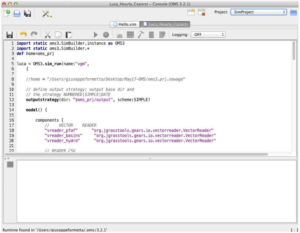
Figure 1.
The OMS Console: OMS components can be linked and executed or automatically calibrated.
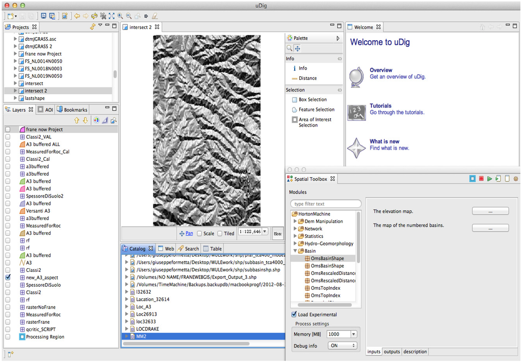
Figure 2.
The uDig GIS interface: (i) the layer view (on the left) where maps are loaded to be visualized (ii) the map view (in the center) allows us to visualize, modify, and query rasters and vectors; the Spatial Toolbox on the right allows the user to execute OMS components.
2.2. The GEOtop Model
The GEOtop model ([8,11]) was chosen mainly because the model simultaneously solves the coupled water, energy, and snow mass balance equations at watershed scales, taking into account vertical and lateral soil variability. The model is open-source, and its integration into the OMS modeling framework is useful for testing and demonstrating the non-invasiveness of the modeling framework [12].
GEOtop is a three-dimensional (3-D), physically based, spatially distributed, finite-volume model that performs water and energy budget calculations. It models saturated and unsaturated subsurface flows, surface runoff, channel flows, and turbulent fluxes across the soil-atmosphere interface (e.g., latent and sensible heat fluxes), and it calculates the discharge at the outlet of the basin. In GEOtop, the heat and water flow equations are linked in a time-lagged manner (e.g., [21]) and are not fully coupled numerically. This ensures a feasible computational time by reducing the numeric complexity. GEOtop takes into account the complex topography of a watershed by using inputs such as a digital elevation model, aspect, local slope, and sky view factor [22] maps when simulating each finite-volume cell of the basin. Moreover the model needs meteorological forcing data such as precipitation, air temperature, solar radiation, and relative humidity. GEOtop simulates surface and subsurface water flows, and it solves the Richards equation in a fully 3-D mode. Simulated state variables include 3-D soil temperature and moisture.
GEOtop estimates the distribution of numerous hydro-meteorological variables including surface temperature, radiative fluxes, and heat fluxes into the soil ([23,24]). Furthermore, GEOtop is able to estimate snow depth, snow-surface temperature, snow water equivalent, and snow density for each grid cell by taking into account the snow metamorphism ([11,25]). These factors make it suitable for the present application to a continental climate with seasonal snow events and associated snowpack dynamics.
2.3. Integration of GEOtop with OMS
In this study, OMS is used with the GEOtop legacy code, which was developed in the C/C++ programming language without using object-oriented language features. The integration of GEOtop into OMS is independent of model complexity, source code programming language, and operating system used. For this reason it can be applied to every kind of environmental model.
Before introducing the steps of the model integration we introduce the concept of the Model.input file (or files). It represents one of more files containing the model’s parameter values such as simulation parameters (start date, end date, time step), numerical parameters (tolerances, maximum iteration number), and physical process parameters (for a subsurface flow model these parameters could be saturated hydraulic conductivity, water retention parameters, etc.). A snapshot of the GEOtop Model.input file is presented in Appendix A.
The procedure of GEOtop integration in OMS follows two main steps besides the model installation:
- Create a template of the Model.input file, where each model parameter is assigned a value that can be accessed and modified. This is performed by the OMS keyword Param_name=${Param_value}, which dynamically substitutes the Param_name with the parameter Param_value.
- Create a Java class named ModelRun.java that receives model parameters as input, creates a new Model.input file by using the template (point 1), and executes the model.
2.4. Goals of Integration
There are several reasons for integrating GEOtop into OMS. The terrain-based structure of GEOtop allows for seamless integration with a GIS system. Version 1.3.1 of uDig (Figure 2), with its embedded Spatial Toolbox, is already integrated with OMS, and uDig runs under different operating systems (Windows, Mac OS/X, and Linux). uDig is internet-oriented and supports geospatial standards such as Web Feature Services (WFS), Web Map Services (WMS), and Web Coverage Services (WCS). De facto standards such as GeoRSS, KML, and tiles are also supported. With such an underlying platform, the integration of GEOtop into OMS allows users to create GEOtop input maps automatically using uDig. GEOtop output maps are generated and visualized within the uDig GIS, and the model is executed via the Spatial Toolbox where spatial model outputs are displayed as maps. This process is illustrated schematically in Figure 3 as the Visualization Process.
OMS also provides tools for automatic calibration of parameters in any OMS component or model. The calibration algorithms available in OMS make it similar to other available software such as PEST [26] or UCODE [27] or the Jupieter API [28]. As a framework for environmental model development, however, OMS allows users to develop, parameterize, and evaluate environmental models providing a set of services such as multithreading, implicit parallelism, interconnection of models, and a GIS-based system. In terms of informatics, OMS is much more flexible than the abovementioned systems. Code modification and inspection, as well as replicability of numerical results, are facilitated using OMS.
Figure 3 shows the OMS Calibration Process. The method we used in this study for GEOtop calibration was LUCa [29] presented in Appendix B. LUCa is a multiple-objective, stepwise, automated procedure based on the Shuffled Complex Evolution global search algorithm [30]. GEOtop parameters, parameter default values, and the hydraulic and geotechnical soil characteristics were also declared as OMS parameters to make them accessible for use by any OMS calibration algorithm.
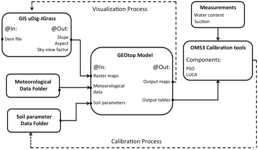
Figure 3.
The GEOtop model is integrated in the OMS framework, as represented in this schematic flow chart. The uDig JGrass GIS is used to create the input raster maps and visualize the output (Visualization Process). Moreover, GEOtop can use the automatic calibration algorithms implemented in OMS. Parameters such as soil hydraulic parameters can be optimized to reproduce measurement data using Particle Swarm Optimization (PSO) or LUCa (based on the Shuffle Complex Evolution method).
In the past, automated calibration of a distributed hydrological model was generally avoided due to the lack of distributed observation and high computational cost. However, with the increasing power of computers, this has become less of an issue. Also, the OMS framework addresses the latter issue by providing transparent use of modern multicores processors via a cloud services platform [12]. GEOtop can also exploit other sets of tools that are included in the NewAge models ([17,19]), like “goodness-of-fit” analysis. Hence, the direct comparison of different modeling solutions is feasible within the same framework using different kinds of meteorological interpolation algorithms, such as ordinary kriging, detrended kriging, or inverse distance weighting.
The GEOtop executable file was wrapped into an OMS component and all platform-specific binaries for various operating systems were bundled with it. Its original input/output structure was modified and the integration result is presented in Figure 3. After reading the meteorological input data (i.e., rainfall, air temperature, and relative humidity), the GEOtop OMS component is executed using the OMS Console (Figure 1). Finally, output maps of soil moisture and temperature are generated directly into uDig. The raster input maps are computed by uDig. By using an OMS simulation script, maps such as aspect, slope, and sky view factor are created as input to GEOtop.
3. Case Study of a GEOtop Application in OMS
A case study was performed to evaluate the model integration as presented in the previous sections and to illustrate model results. The application is a simulation of daily soil moisture (SM) and soil temperature (ST) at selected landscape positions in the Drake watershed (56 ha) within the lower Cache la Poudre river basin (near Severance, Colorado, USA).
The field site has been described and studied previously regarding terrain analysis [31], spatial scaling of infiltration rates [32], temporal dynamics of measured soil moisture at different landscape positions [33], one-dimensional simulations of soil moisture ([14,34]), and interrelationships between terrain and wheat development [35]. The watershed defined by an outlet at the eastern edge of the cropped field has an elevation range of 1559–1588 m, a mean annual precipitation of approximately 350 mm, and a mean annual evapotranspiration of approximately 1200 mm. Soils were described by soil horizon at the soil water probe locations [33]. Soil texture changes with depth, ranging from fine sandy loam to clay loam across the watershed. The management of the field is based on a winter wheat-fallow rotation ([33,36]).
The meteorological data were collected on-site, as described in [14]. Data for the period of simulations reported here (September 2002–August 2003) were collected using a weighing rain gauge constructed at the USDA-ARS laboratory in Tucson, AZ and a micro-meteorological station (Pessl™ Instruments Weiz, Austria) for incoming solar radiation, air temperature, relative humidity, and wind speed. Sensor measurements were recorded at 12-min or finer intervals, then averaged to provide daily values as model inputs. Four Sentek™ SM measurement probes (Stepney SA, Australia) were included in this study: C1, C2, C3, and C4, each with sensors at four depths: 300, 600, 900 and 1200 mm. Moreover, for each location ST was measured at 300 and 600 mm depths. Figure 4 shows the Drake watershed and the locations of the four probes.
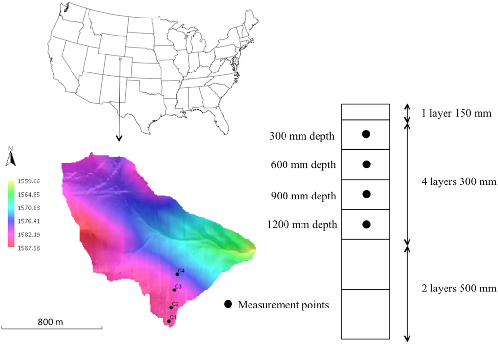
Figure 4.
Drake watershed digital elevation model and measurement stations. The soil profile shows model layers and depths of automated SM measurements. Sensors are centered on the depths shown, with measured intervals of approximately 100 mm each ([33,37]).
The objective of the case study was to demonstrate the benefits of porting GEOtop into the OMS system. One benefit is the facilitation of the automatic calibration algorithms in OMS. Calibrated results for simulated SM and ST at different depths are presented in the next subsections. Here, soil parameters were allowed to vary with depth, but were uniform across the watershed. Full heterogeneity is possible in GEOtop, but runtime and non-uniqueness of parameter sets made such work beyond our current scope.
3.1. Model Setup
The following data were used for model input:
- A digital elevation model of the area with 5-m horizontal grid spacing;
- one year (1 September 2002 to 31 August 2003) of measured daily rainfall, air temperature, relative humidity, and incoming solar radiation;
- Soil-specific hydraulic and geotechnical parameters such as saturated and residual water content, lateral and vertical hydraulic conductivity, and van Genuchten and Mualem parameters of the soil water characteristic curve, represented by eight layers as shown in Figure 4;
- GEOtop input maps (slope, aspect, and sky view factor) created with OMS simulation scripts using uDig geo-processing components.
The resulting model was executed using the OMS Console. Both energy and water balance were computed, and simulated SM and ST results were compared with measurements. GEOtop spatial outputs of SM were displayed as maps using uDig (Figure 2).
3.2. Model Results
The objective was to calibrate GEOtop in each location using the LUCa component in OMS. An optimal parameter set was fit to both SM (at 300, 600, 900, and 1200 mm depths) and ST (at 300 and 600 mm depths) for each location (C1, C2, C3, and C4). The four optimal parameter sets (named Par_C1, Par_C2, Par_C3, and Par_C4) are presented in Table 1, which contains the parameters related to the water budget (Mualem and van Genuchten parameters) with different values for each soil layer. All parameters were uniform in the horizontal direction for these simulations. The objective function was the Kling–Gupta Efficiency (KGE), presented in [38]:
In KGE, simulated (s) and measured (m) time series were compared simultaneously in three aspects within Equation (1): (i) correlation coefficient (R), (ii) variability error (), and (iii) bias error (). The mean values of simulated and measured time series are and , respectively, and and are the standard deviations of simulated and measured time series. The range of KGE values is , and its optimal value is 1.0, which means that the model fits the measurements perfectly. Moreover, we use the root mean square error (RMSE) to measure the model performance.
In the second part of the case study, each of the parameter sets was used to predict SM and ST in the locations where they were not calibrated (i.e., cross-evaluation). The set Par_C1, estimated by using measurement data in the location C1, was used to predict SM and ST in C2, C3, and C4. The same procedure was applied for parameter sets Par_C2, Par_C3, and Par_C4. Results in terms of both KGE and RMSE values are presented in Table 2. Each column of the table represents the optimal parameter set used in the simulations (Par_C1, Par_C2, Par_C3, and Par_C4). Each row of the table represents the hydrological state variable, SM or ST, at the locations C1, C2, C3, or C4 and depths 300, 600, 900, or 1200 mm for which the comparison is performed.
Figure 5 and Figure 6 show the simulation results from a qualitative point of view. For each location and for each depth, the measured data (blue line), the simulated results provided by the parameter set estimated in this location (solid black line), and the results provided by the parameter estimated in the other three locations (dashed and dotted black lines) are presented.

Table 1.
Optimal parameter sets for the four locations estimated by using the LUCa calibration algorithm. Dz (mm) is the depth of each soil layers from ground level, Kh and Kv (mm/s) are the lateral and the vertical hydraulic conductivities, respectively, θr and θs (m3·m−3) are the residual and saturated water contents, respectively, and α (m−1) and n are the van Genuchten parameters.
| Dz (mm) | Kh (mm/s) | Kv (mm/s) | θr | θs | α (m−1) | n (-) |
|---|---|---|---|---|---|---|
| Par_C1 | ||||||
| 150 | 0.029 | 0.061 | 0.061 | 0.533 | 5.4 | 1.819 |
| 450 | 0.076 | 0.027 | 0.061 | 0.570 | 4.0 | 1.474 |
| 750 | 0.055 | 0.053 | 0.044 | 0.539 | 5.2 | 1.384 |
| 1050 | 0.054 | 0.023 | 0.066 | 0.550 | 5.6 | 1.455 |
| 1350 | 0.049 | 0.019 | 0.071 | 0.536 | 5.9 | 1.340 |
| 1850 | 0.045 | 0.039 | 0.069 | 0.478 | 4.0 | 1.556 |
| 2350 | 0.083 | 0.055 | 0.052 | 0.528 | 3.6 | 1.246 |
| Par_C2 | ||||||
| 150 | 0.031 | 0.005 | 0.070 | 0.519 | 2.1 | 1.148 |
| 450 | 0.061 | 0.015 | 0.067 | 0.577 | 3.5 | 1.337 |
| 750 | 0.045 | 0.021 | 0.066 | 0.580 | 6.0 | 1.351 |
| 1050 | 0.051 | 0.032 | 0.087 | 0.473 | 5.0 | 1.529 |
| 1350 | 0.023 | 0.074 | 0.087 | 0.448 | 3.3 | 1.758 |
| 1850 | 0.054 | 0.061 | 0.018 | 0.499 | 4.3 | 1.368 |
| 2350 | 0.078 | 0.048 | 0.086 | 0.449 | 3.4 | 1.740 |
| Par_C3 | ||||||
| 150 | 0.067 | 0.028 | 0.028 | 0.560 | 4.8 | 1.269 |
| 450 | 0.065 | 0.063 | 0.070 | 0.583 | 3.3 | 1.346 |
| 750 | 0.084 | 0.017 | 0.055 | 0.519 | 3.6 | 1.392 |
| 1050 | 0.049 | 0.014 | 0.067 | 0.503 | 5.1 | 1.469 |
| 1350 | 0.039 | 0.043 | 0.098 | 0.490 | 4.6 | 1.731 |
| 1850 | 0.027 | 0.088 | 0.055 | 0.530 | 4.8 | 1.199 |
| 2350 | 0.014 | 0.056 | 0.084 | 0.483 | 2.9 | 1.534 |
| Par_C4 | ||||||
| 150 | 0.095 | 0.036 | 0.038 | 0.497 | 2.7 | 1.198 |
| 450 | 0.044 | 0.049 | 0.095 | 0.434 | 3.8 | 1.366 |
| 750 | 0.067 | 0.021 | 0.076 | 0.565 | 1.4 | 1.387 |
| 1050 | 0.032 | 0.031 | 0.073 | 0.525 | 5.6 | 1.764 |
| 1350 | 0.078 | 0.082 | 0.095 | 0.523 | 4.5 | 1.849 |
| 1850 | 0.033 | 0.006 | 0.044 | 0.568 | 5.0 | 1.438 |
| 2350 | 0.010 | 0.032 | 0.038 | 0.421 | 6.4 | 1.243 |
The model is able to simulate the main wetting front and stable patterns of the SM profile both at low-saturation (September–March) and to a better degree at high-saturation (March–August) periods. This is also confirmed by the indices of goodness-of-fit reported in Table 2. Generally, the best performances were achieved by using the parameter set estimated in the same locations where calibration is performed (e.g., parameter set Par_C1 gives the best results in location C1). For a given depth, the optimal parameter set at other locations may show better results in comparison to the optimal parameter set that was calibrated for the given location. For example, the optimal parameter set of Par_C2 showed smaller RMSE (4.03) for SM_C1_300 than for the optimal parameter set Par_C1 (5.02) (see Table 2). Moreover, the simulated SM at probe C1, 300 mm depth using Par_C2 reproduced the measured SM better during March–April compared with the simulation using Par_C1 (Figure 5). This happens only for SM_C1_300, but in the other locations the RMSE values using Par_C2 are much higher than using Par_C1 (4.30 vs. 2.10 for SM_C1_600, 2.2 vs. 7.6 for SM_C1_900, and 1.08 vs. 6.4 for SM_C1_1200). This example shows how the parameter set Par_C1 is “globally” optimal for the site C1, where the term “globally” indicates the fact that the algorithm simultaneously optimizes the parameters in the four locations C1_300, C1_600, C1_900, and C1_1200.
In a fully three-dimensional calibration exercise (beyond the present scope), we expect GEOtop to capture soil water dynamics at different landscape positions synoptically using one parameter set. [14] showed a decrease in goodness-of-fit to SM at downslope positions (high contributing areas) using the AgroEcoSystem (AgES) model for vertical SM flow only, which indicates that three-dimensional flowpaths are important.
Table 2.
Kling-Gupta Efficiency (KGE) coefficients and root mean squared error (RMSE) values quantify the model goodness of fit. The coefficients are reported for each optimal parameter set (Par_C1, Par_C2, Par_C3, and Par_C4) calibrated in each location (C1, C2, C3, and C4, respectively) and for each depth (300, 600, 900, and 1200 mm), for soil moisture (SM, m3·m−3 × 100%), and for soil temperature (ST, °C).
| Measure of Fit | KGE | RMSE | ||||||
|---|---|---|---|---|---|---|---|---|
| Parameter Set | Par_C1 | Par_C2 | Par_C3 | Par_C4 | Par_C1 | Par_C2 | Par_C3 | Par_C4 |
| SM_C1_300 | 0.84 | 0.74 | 0.73 | 0.50 | 5.02 | 4.03 | 5.12 | 6.33 |
| SM_C1_600 | 0.96 | 0.82 | 0.91 | 0.63 | 2.10 | 4.30 | 2.40 | 5.73 |
| SM_C1_900 | 0.95 | 0.11 | 0.63 | 0.52 | 2.20 | 7.64 | 4.50 | 4.80 |
| SM_C1_1200 | 0.98 | −0.13 | 0.14 | 0.43 | 1.08 | 9.00 | 7.14 | 5.63 |
| ST_C1_300 | 0.86 | 0.36 | 0.87 | 0.78 | 1.86 | 6.42 | 1.56 | 2.19 |
| ST_C1_600 | 0.97 | 0.39 | 0.94 | 0.89 | 1.21 | 5.77 | 1.32 | 1.40 |
| SM_C2_300 | 0.58 | 0.91 | 0.72 | 0.32 | 7.30 | 4.61 | 4.65 | 9.32 |
| SM_C2_600 | 0.79 | 0.91 | 0.81 | 0.75 | 5.15 | 2.16 | 4.19 | 5.43 |
| SM_C2_900 | 0.06 | 0.92 | 0.55 | 0.56 | 6.19 | 1.23 | 2.62 | 3.85 |
| SM_C2_1200 | −3.08 | 0.72 | 0.82 | −0.55 | 7.02 | 1.71 | 1.88 | 2.35 |
| ST_C2_300 | 0.23 | 0.79 | 0.20 | 0.28 | 7.47 | 2.57 | 7.70 | 6.85 |
| ST_C2_600 | 0.25 | 0.91 | 0.21 | 0.30 | 7.10 | 1.54 | 7.44 | 6.50 |
| SM_C3_300 | 0.80 | 0.79 | 0.93 | 0.49 | 5.21 | 3.26 | 2.63 | 6.60 |
| SM_C3_600 | 0.91 | 0.83 | 0.96 | 0.65 | 3.34 | 3.03 | 1.94 | 6.15 |
| SM_C3_900 | 0.50 | 0.25 | 0.98 | 0.80 | 4.54 | 4.36 | 1.08 | 2.37 |
| SM_C3_1200 | −2.79 | −0.03 | 0.85 | 0.07 | 6.65 | 2.23 | 0.76 | 1.34 |
| ST_C3_300 | 0.85 | 0.36 | 0.90 | 0.84 | 1.90 | 6.36 | 1.54 | 1.90 |
| ST_C3_600 | 0.94 | 0.37 | 0.96 | 0.91 | 1.32 | 6.05 | 1.33 | 1.44 |
| SM_C4_300 | 0.15 | −0.33 | 0.17 | 0.65 | 9.67 | 9.61 | 7.07 | 7.90 |
| SM_C4_600 | 0.80 | 0.69 | 0.80 | 0.94 | 3.95 | 5.88 | 4.08 | 1.76 |
| SM_C4_900 | −0.18 | 0.35 | 0.50 | 0.93 | 7.05 | 2.80 | 3.17 | 1.19 |
| SM_C4_1200 | −2.44 | −0.05 | 0.79 | 0.81 | 6.63 | 2.12 | 0.77 | 0.96 |
| ST_C4_300 | 0.85 | 0.35 | 0.89 | 0.85 | 1.74 | 6.32 | 1.31 | 1.68 |
| ST_C4_600 | 0.95 | 0.37 | 0.96 | 0.94 | 1.18 | 5.86 | 1.23 | 1.12 |
Results presented in Figure 5 and Figure 6 illustrate the processes of partial saturation and de-saturation. The simulation period (September–August) was selected in order to show the change in saturation from around 0.22 (m3·m−3) to around 0.40 (m3·m−3). This was mainly due to intense early-season rainfall wetting fallow soils that were relatively dry over the winter due to crop water uptake in the previous year. Before and after the main wetting front, the model simulates relatively steady moisture states, which is an improvement over the dynamics at high moisture states simulated previously with another numerical model [34]. However, some of the high-frequency temporal dynamics are not captured fully with GEOtop in this study. For example the timings of the soil moisture peaks are not precise at 300 mm depth in locations C1 and C2; this could be due to sub-optimal estimation of the saturated hydraulic conductivity for these layers or to the spatial variability of rainfall that we neglected in our application.
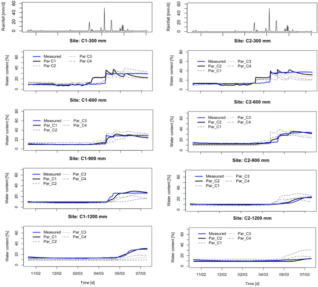
Figure 5.
Soil moisture dynamics at different depths (300, 600, 900 and 1200 mm) in locations C1 and C2. The blue bold lines are the measured data. The black lines are simulated SM values computed by using different parameters set (Par_C1, Par_C2, Par_C3, and Par_C4) as specified in the legend.
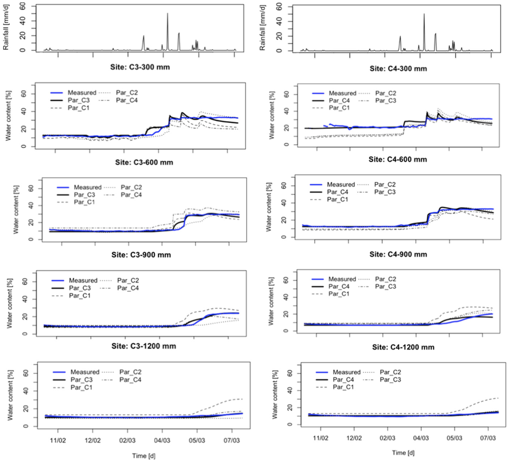
Figure 6.
Soil moisture dynamics at different depths (300, 600, 900 and 1200 mm) in locations C3 and C4. The blue bold lines are the measured data. The black lines are simulated SM values computed by using different parameters set (Par_C1, Par_C2, Par_C3, and Par_C4) as specified in the legend.
Figure 7 presents the plots of the soil temperature (ST) for each location, depth, and parameter set used in the simulation. The model was able to simulate the temporal dynamics of ST well. The results are satisfactory in all locations not only from a qualitative point of view but also from a quantitative point of view (Table 2). Seasonality of ST is generally captured well, because it is driven directly by the input air temperature. Variations over shorter time periods are driven by air temperature (conduction), insolation (radiative heating), and heat transport in water (convection). Despite the implied complexity and interactions between processes, GEOtop captured many events well using the at-site calibrations. Variations among calibrations show the potential spatial variability within this small watershed.
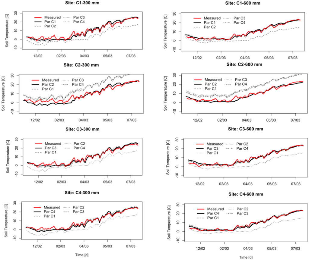
Figure 7.
Soil temperature dynamics at different depths (300 and 600 mm) in locations C1, C2, C3, and C4. The red bold lines are the measured data. The black lines are simulated ST values computed by using a different parameters set (Par_C1, Par_C2, Par_C3, and Par_C4), as specified in the legend.
4. Conclusions
This paper presented an integration of the fully distributed hydrological model GEOtop into the OMS framework. The three main goals of the work were accomplished:
- (1)
- The uDig GIS was used to compute input maps and provide output visualization for GEOtop (Figure 2).
- (2)
- The GEOtop model was linked to OMS to execute automatic calibration, sensitivity analysis, and meteorological interpolation tools.
- (3)
- Integrating GEOtop into OMS enhanced the modeling library, which includes other lumped and semi-distributed hydrological models such as PRMS, AgES-W, and NewAge. Modelers may select the appropriate model according to their needs and the processes to be simulated.
Finally, an application was presented as a case study. The OMS LUCa calibration algorithm was applied to optimize some of the model parameters based on measured data at different locations within the Drake watershed. Model results were compared with measured data from both qualitative and quantitative points of view. Simulated SM compared favorably with previous one-dimensional simulations ([14,34]) and soil temperature was generally reproduced well. Parameter values in GEOtop were allowed to vary only with depth (no lateral spatial variability). The application shows the importance of automated calibration and how it enhances the accuracy of physics-based models. The same model configuration presented in this paper could be used in future work using distributed data from remote sensing as observations. Moreover, future work could explore three-dimensional variability of parameters, which should lead to improved model fits across landscape positions, and influence of soil depth variability on soil moisture spatial distribution. This application illustrates the flexibility of the OMS system for model integration and the advantages gained by a model such as GEOtop from the integration with calibration tools available in OMS.
Acknowledgments
This research was supported by the Ambito/Settore AMBIENTE E SICUREZZA (PON01_01503) project. Our special thanks go to Luis Garcia of the University of Vermont, formerly Head of the Department of Civil & Environmental Engineering at Colorado State University. Rob Erskine, USDA-ARS, assisted with collection and processing of the field data.
Author Contributions
Giuseppe Formetta, Timothy R. Green, Giovanna Capparelli, Riccardo Rigon, and Olaf David conceived and designed the experiments; Giuseppe Formetta performed the experiments; Giuseppe Formetta, Timothy R. Green and Giovanna Capparelli analyzed the data; Giuseppe Formetta, Olaf David, Riccardo Rigon, Timothy R. Green and Giovanna Capparelli contributed materials/analysis tools; Giuseppe Formetta and Timothy R. Green wrote the paper.
Conflicts of Interest
The authors declare no conflict of interest.
Appendix A
!*******************************
!******* CONFIGURATION *********
!*******************************
TimeStepEnergyAndWater = ${TimeStepEnergyAndWater_value}
InitDateDDMMYYYYhhmm = ${InitDateDDMMYYYYhhmm_value}
EndDateDDMMYYYYhhmm = ${EndDateDDMMYYYYhhmm_value}
EnergyBalance =${EnergyBalance_value}
WaterBalance = ${WaterBalance_value}
!*******************************
!********* GEOGRAPHY ***********
!*******************************
Latitude = ${Latitude_value}
Longitude = ${Longitude_value}
!*******************************
!****** METEO STATIONS *********
!*******************************
NumberOfMeteoStations= ${NumberOfMeteoStations_value}
MeteoStationCoordinateX= ${MeteoStationCoordinateX_value}
MeteoStationCoordinateY= ${MeteoStationCoordinateY_value}
MeteoStationElevation= ${MeteoStationElevation_value}
!*******************************
!**** BOUNDARY AND INITIAL *****
!******  CONDITION STATIONS *****
!*******************************
InitWaterTableHeightOverTopoSurface= ${InitWaterTableHeightOverTopoSurface_value}
FreeDrainageAtLateralBorder= ${FreeDrainageAtLateralBorder_value}
FreeDrainageAtBottom= ${FreeDrainageAtBottom_value}
!*******************************
!******* INPUT MAPS ************
!*******************************
DemFile = ${DemFile_value}
MeteoFile = ${MeteoFile_value}
LandCoverMapFile = ${LandCoverMapFile_value}
SkyViewFactorMapFile = ${SkyViewFactorMapFile_value}
SlopeMapFile = ${SlopeMapFile_value}
AspectMapFile = ${AspectMapFile_value}
RiverNetwork = ${RiverNetwork_value}
Appendix B
The LUCa calibration algorithm [29] in OMS is a multiple-objective, stepwise, automated procedure for model calibration. LUCa is based on two concepts: a search algorithm and the objective function(s) (OF) to evaluate model performance. The LUCa global searching algorithm is the Shuffled Complex Evolution (SCE, [30]). The OF can be selected by the user from a set of classical predefined OF. In our example we selected the Kling–Gupta Efficiency OF.
The LUCa algorithm is based on two important concepts: steps and rounds. A step is associated with the optimization of a specific parameter set, which contains one or more parameter values. A round consists of the execution of one or more steps. The selected parameters are calibrated for each calibration step. Completion of the user-designated number of steps constitutes a round. A LUCa run configured with one step and one round represents a classic SCE.
Lastly, LUCa allows simultaneous optimization of different objective functions by assigning a weight to each OF. In our application, we used the same weight for each optimized objective function. [14] applied LUCa to estimate vertically layered soil parameters and other model parameters in AgES to fit soil moisture profiles at different landscape positions.
References
- Freeze, R.A.; Harlan, R.L. Blueprint for a physically-based, digitally-simulated hydrologic response model. J. Hydrol. 1969, 9, 237–258. [Google Scholar] [CrossRef]
- Abbott, M.B.; Bathurst, J.C.; Cunge, J.A.; O’connell, P.E.; Rasmussen, J. An introduction to the European Hydrological System—Systeme Hydrologique Europeen,“SHE”, 2: Structure of a physically-based, distributed modelling system. J. Hydrol. 1986, 87, 61–77. [Google Scholar] [CrossRef]
- Maxwell, R.M.; Putti, M.; Meyerhoff, S.; Delfs, J.-O.; Ferguson, I.M.; Ivanov, V.; Kim, J.; Kolditz, O.; Kollet, S.J.; Kumar, M.; et al. Surface-subsurface model intercomparison: A first set of benchmark results to diagnose integrated hydrology and feedbacks. Water Resour. Res. 2014, 50, 1531–1549. [Google Scholar] [CrossRef]
- Furman, A. Modeling coupled surface-subsurface flow processes: A review. Vadose Zone J. 2008, 7, 741–756. [Google Scholar] [CrossRef]
- Paniconi, C.; Marrocu, M.; Putti, M.; Verbunt, M. Newtonian nudging for a Richards equation-based distributed hydrological model. Adv. Water Resour. 2003, 26, 161–178. [Google Scholar] [CrossRef]
- Garrote, L.; Bras, R.L. A Distributed Model for Real-time Flood Forecasting using Digital Elevation Models. J. Hydrol. 1995, 167, 279–306. [Google Scholar] [CrossRef]
- Zehe, E.; Blöschl, G. Predictability of hydrologic response at the plot and catchment scales: Role of initial conditions. Water Resour. Res. 2004, 40. [Google Scholar] [CrossRef]
- Rigon, R.; Bertoldi, G.; Over, T.M. GEOtop: A distributed hydrological model with coupled water and energy budgets. J. Hydrometeorol. 2006, 7, 371–388. [Google Scholar] [CrossRef]
- Wang, L.; Koike, T.; Yang, K.; Yeh, P.J.F. Assessment of a distributed biosphere hydrological model against streamflow and MODIS land surface temperature in the upper Tone River Basin. J. Hydrol. 2009, 377, 21–34. [Google Scholar] [CrossRef]
- Niu, G.-Y.; Paniconi, C.; Troch, P.A.; Scott, R.L.; Durcik, M.; Zeng, X.; Huxman, T.; Goodrich, D.C. An integrated modelling framework of catchment-scale ecohydrological processes: 1. Model description and tests over an energy-limited watershed. Ecohydrology 2014, 7, 427–429. [Google Scholar] [CrossRef]
- Endrizzi, S.; Gruber, S.; Dall’Amico, M.; Rigon, R. GEOtop 2.0: Simulating the combined energy and water balance at and below the land surface accounting for soil freezing, snow cover and terrain effects. Geosci. Model Dev. Discuss. 2013, 6, 6279–6341. [Google Scholar] [CrossRef]
- David, O.; Ascough, J.C.; Lloyd, W.; Green, T.R.; Rojas, K.W.; Leavesley, G.H.; Ahuja, L.R. A software engineering perspective on environmental modeling framework design: The Object Modeling System. Environ. Model. Softw. 2013, 39, 201–213. [Google Scholar] [CrossRef]
- Formetta, G.; Antonello, A.; Franceschi, S.; David, O.; Rigon, R. Hydrological modelling with components: A GIS-based open-source framework. Environ. Model. Softw. 2014, 55, 190–200. [Google Scholar] [CrossRef]
- Green, T.R.; Erskine, R.H.; Coleman, M.L.; David, O.; Ascough, J.C.; Kipka, H. The AgroEcoSystem (AgES) response-function model simulates layered soil-water dynamics in semi-arid Colorado: Sensitivity and calibration. Vadose Zone J. 2015, 14. [Google Scholar] [CrossRef]
- Ascough, J.C.; David, O.; Krause, P.; Heathman, G.C.; Kralisch, S.; Larose, M.; Ahuja, L.R.; Kipka, H. Development and application of a modular watershed-scale hydrologic model using the Object Modeling System: Runoff response evaluation. Trans. ASABE 2012, 55, 117–135. [Google Scholar] [CrossRef]
- David, O.; Markstrom, S.; Rojas, K.; Ahuja, L.; Schneider, I. The Object Modeling System, Agricultural System Models in Field Research and Technology Transfer; CRC Press: Boca Raton, FL USA, 2002; pp. 317–331. [Google Scholar]
- Formetta, G.; Mantilla, R.; Franceschi, S.; Antonello, A.; Rigon, R. The JGrass-Newage system for forecasting and managing the hydrological budgets at the basin scale: Models of flow generation and propagation/routing. Geosci. Model Dev. 2011, 4, 943–955. [Google Scholar] [CrossRef]
- Leavesley, G.H.; Markstrom, S.L.; Viger, R.J. USGS Modular Modeling System (MMS)-Precipitation-Runoff Modeling System (PRMS). In Watershed Models; CRC Press: Boca Raton, FL, USA, 2006; pp. 159–177. [Google Scholar]
- Formetta, G.; Rigon, R.; Chávez, J.L.; David, O. Modeling shortwave solar radiation using the JGrass-NewAge system. Geosci. Model Dev. 2013, 6, 915–928. [Google Scholar] [CrossRef]
- Lloyd, W.; David, O.; Ascough, J.C.; Rojas, K.W.; Carlson, J.R.; Leavesley, G.H.; Krause, P.; Green, T.R.; Ahuja, L.R. Environmental modeling framework invasiveness: Analysis and implications. Environ. Model. Softw. 2011, 26, 1240–1250. [Google Scholar] [CrossRef]
- Panday, S.; Huyakorn, P.S. A fully coupled physically-based spatially-distributed model for evaluating surface/subsurface flow. Adv. Water Resour. 2004, 27, 361–382. [Google Scholar] [CrossRef]
- Zakšek, K.; Oštir, K.; Kokalj, Ž. Sky-view factor as a relief visualization technique. Remote Sens. 2012, 3, 398–415. [Google Scholar] [CrossRef]
- Bertoldi, G.; Rigon, R.; Over, T.M. Impact of watershed geomorphic characteristics on the energy and water budgets. J. Hydrometeorol. 2006, 7, 389–403. [Google Scholar] [CrossRef]
- Gubler, S.; Endrizzi, S.; Gruber, S.; Purves, R.S. Sensitivities and uncertainties of modeled ground temperatures in mountain environments. Geosci. Model Dev. 2013, 6, 1319–1336. [Google Scholar] [CrossRef]
- Dall’Amico, M.; Endrizzi, S.; Gruber, S.; Rigon, R. An energy-conserving model of freezing variably-saturated soil. Cryosphere 2011, 5, 469–484. [Google Scholar] [CrossRef]
- Doherty, J.E.; Hunt, R.J. Approaches to Highly Parameterized Inversion: A Guide to Using PEST for Groundwater-Model Calibration; U.S. Department of the Interior, U.S. Geological Survey: Reston, VA, USA, 2010.
- Poeter, E.P.; Hill, M.C. UCODE, a computer code for universal inverse modeling. Comput. Geosci. 1999, 25, 457–462. [Google Scholar] [CrossRef]
- Banta, E.R.; Poeter, E.P.; Doherty, J.E.; Hill, M.C. JUPITER: Joint Universal Parameter Identification and Evaluation of Reliability—An Application Programming Interface (API) for Model Analysis; U.S. Geological Survey: Reston, VA, USA, 2006.
- Hay, L.E.; Leavesley, G.H.; Clark, M.P.; Markstrom, S.L.; Viger, R.J.; Umemoto, M. Step-Wise, Multiple-Objective Calibration of a Hydrologic Model for a Snowmelt-Dominated Basin. J. Am. Water Resour. Assoc. 2006, 42, 877–890. [Google Scholar] [CrossRef]
- Duan, Q.; Sorooshian, S.; Gupta, V. Effective and efficient global optimization for conceptual rainfall-runoff models. Water Resour. Res. 1992, 28, 1015–1031. [Google Scholar] [CrossRef]
- Erskine, R.H.; Green, T.R.; Ramirez, J.A.; MacDonald, L. Comparison of grid-based algorithms for computing upslope contributing area. Water Resour. Res. 2006, 42. [Google Scholar] [CrossRef]
- Green, T.R.; Dunn, G.H.; Erskine, R.H.; Salas, J.D.; Ahuja, L.R. Fractal analyses of steady infiltration and terrain on an undulating agricultural field. Vadose Zone J. 2009, 8, 310–320. [Google Scholar] [CrossRef]
- Green, T.R.; Erskine, R.H. Measurement and inference of profile soil-water dynamics at different hillslope positions in a semiarid agricultural watershed. Water Resour. Res. 2011, 47. [Google Scholar] [CrossRef]
- Fang, Q.X.; Green, T.R.; Liwang, M.; Erskine, R.H.; Malone, R.W.; Ahuja, L.R. Optimizing soil hydraulic parameters in RZWQM2 under fallow conditions. Soil Sci. Soc. Am. J. 2010, 74, 1887–1993. [Google Scholar] [CrossRef]
- McMaster, G.S.; Green, T.R.; Erskine, R.H.; Edmunds, D.A.; Ascough, J.C. Interrelationships between wheat phenology, thermal time, and landscape position. Agron. J. 2012, 104, 1110–1121. [Google Scholar] [CrossRef]
- Kipka, H.; Green, T.R.; David, O.; Garcia, L.A.; Ascough, J.C.; Arabi, M. Development of the Land-use and Agricultural Management Practice web-Service (LAMPS) for generating crop rotations in space and time. Soil Tillage Res. 2016, 155, 233–249. [Google Scholar] [CrossRef]
- Schwank, M.; Green, T.R.; Mätzler, C.; Benedickter, H.; Flühler, H. Laboratory characterization of a commercial capacitance sensor for estimating permittivity and inferring soil water content. Vadose Zone J. 2006, 5, 1048–1064. [Google Scholar] [CrossRef]
- Gupta, H.; Kling, H.; Yilmaz, K.; Martinez, G. Decomposition of the mean squared error and NSE performance criteria: Implications for improving hydrological modelling. J. Hydrol. 2009, 377, 80–91. [Google Scholar] [CrossRef]
© 2016 by the authors; licensee MDPI, Basel, Switzerland. This article is an open access article distributed under the terms and conditions of the Creative Commons by Attribution (CC-BY) license (http://creativecommons.org/licenses/by/4.0/).