Flood-Runoff in Semi-Arid and Sub-Humid Regions, a Case Study: A Simulation of Jianghe Watershed in Northern China

Abstract

This paper presents a modeling application of surface runoff using the Hydrologic Modelling System (HEC-HMS). A case study was carried out for the Jianghe watershed, a typical semi-arid and sub-humid geo-climatic region in northern China. Two modeling schemes using different descriptive sub-mechanism models provided by HEC-HMS for runoff volume, direct runoff and routing (channel flow) were investigated. The modeling results were compared with historical observation data. This work shows that HEC-HMS can be a suitable modeling tool for specific situations in China. With the appropriate selection of the sub-mechanism models, HEC-HMS can be applied to various situations, including the typical semi-arid and sub-humid conditions in northern China.

1. Introduction

Surface runoff or flood runoff is the flow of water over the ground surface. This happens when soil is fully saturated or heavy rain falls over a short period of time such that it cannot be completely absorbed by the ground surface. Surface runoff plays an important role in the water cycle and resource distribution in geological ecosystems. It also has a direct effect on soil erosion and consequently, flooding. There are many factors that influence surface runoff, including rainfall dynamics, ground geo-topography, types of soil and vegetation, land use and development, etc. [1,2].

In China, the modeling of surface runoff has been studied since the early 1960s. Specific models for different climatic and environmental conditions have been proposed [3], such as the Xinanjiang-model used for the humid regions [4,5,6,7] and the Shanbei-model used for the arid regions in China [3,8]. However, these two models are not able to represent all of the typical geo-climatic characteristics of the vast and diverse territory of China. For example, in northern China, where the climate presents both semi-arid and sub-humid characteristics, the rainfall and runoff processes are much more complicated than those that occur in solely humid or arid regions.

The Hydrologic Modeling System (HEC-HMS) is an integrated modeling and simulation tool for all hydrologic processes of dendritic watershed systems. It consists of different sub-mechanism models for rainfall loss, direct runoff and routing, i.e., the component processes involved in the transfer of rainfall to runoff. This paper reports a case study of the application of the HEC-HMS in the flood modeling of a typical semi-arid and sub-humid region, the Jianghe watershed, in northern China. It aims to investigate the suitability of the sub-mechanism models provided by HEC-HMS and to identify an effective modeling strategy using the appropriate sub-models for flooding processes under these climatic and environmental conditions.

2. Study Area and Data

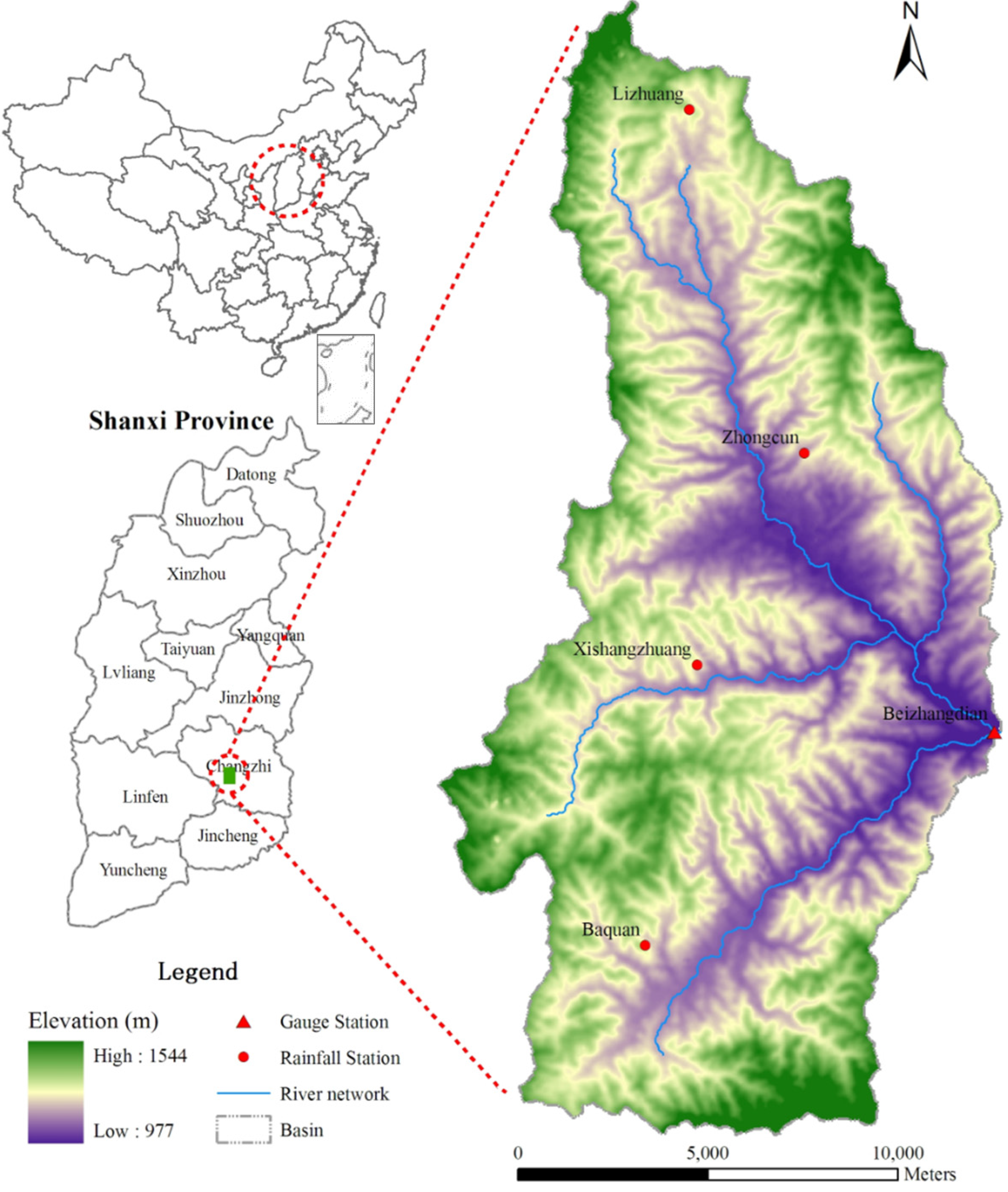
The Jianghe watershed is located in the midwest of Changzhi city, Shanxi Province, China (Figure 1). It comprises a catchment area of about 270 Km², with an elevation range from 977 to 1544 m. The altitude is high in the north, west and south, but low in the east and the center. The watershed is located in a typical semi-arid and sub-humid climatic region in northern China, where the annual average precipitation is approximately 564 mm, with a recorded maximum of 872.2 mm in 1971 and a minimum of 299.1 mm in 1983. The precipitation in a single year varies substantially but typically, intensive rainfalls occur in summer (June to September). The annual average water surface evaporation is about 1775.8 mm and the annual average temperature is about 9.1 °C.

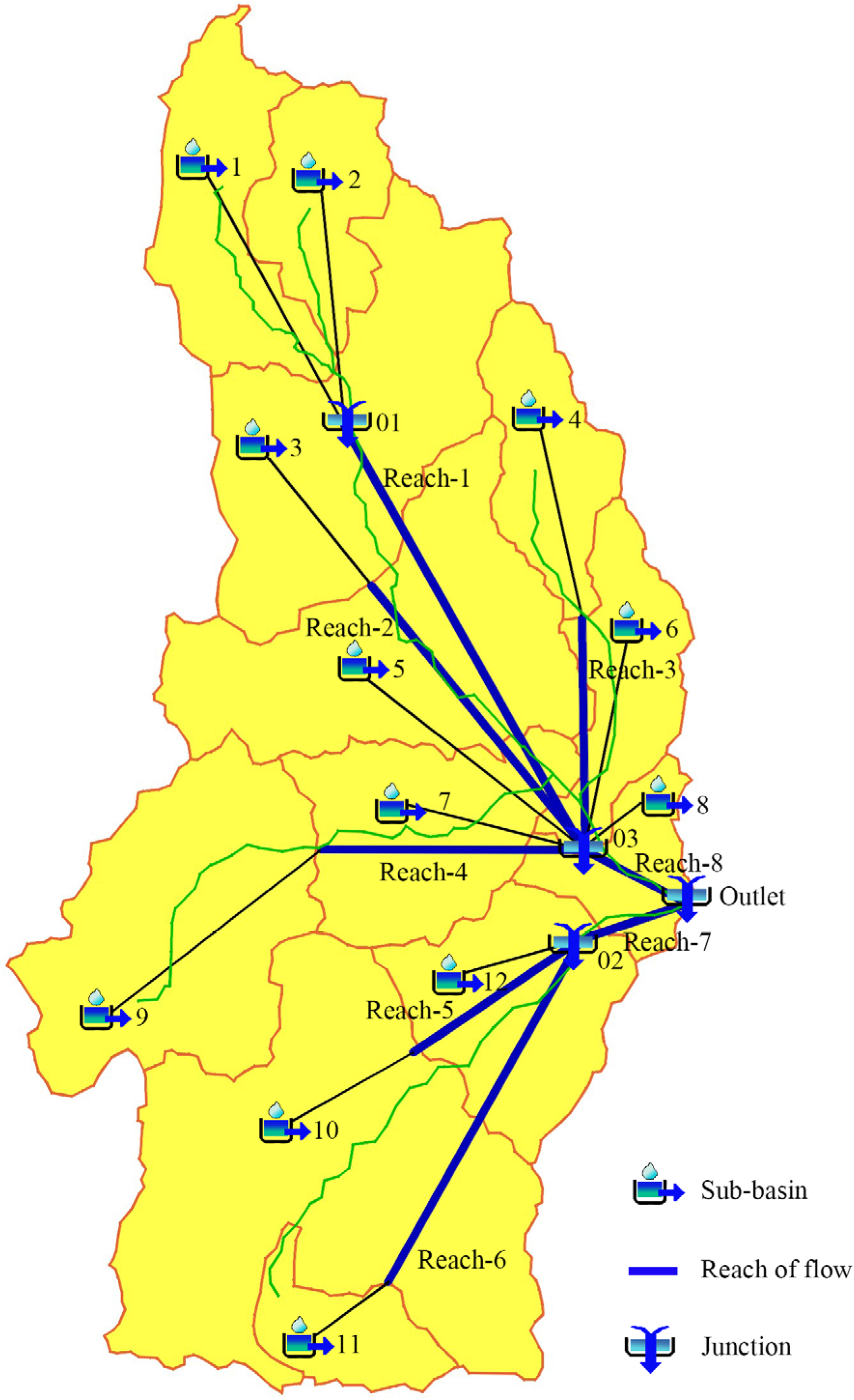
The watershed was discretized into 12 sub-basins as shown in Figure 2. Digital Elevation Model (DEM) data with a 30-m resolution, obtained from the Computer Network Information Center, Chinese Academy of Sciences, were employed to characterize the stream network and the topographic attributes (e.g., area, length and slope) of each sub-basin based on a 1:50,000 topographical map. The characterized topographical data are listed in Table 1.

The land use data were obtained from the United States Geological Survey. The main type of land in the Jianghe watershed is grassland of low to medium coverage, comprising about half of the total area. The other land uses are forest, shrub, open forest and flood plain. The land use data are listed in Table 2. The soil type data were obtained from the China Soil Science Database. The major type in the region is cinnamon soil belonging to the C soil type according to the Soil Conservation Service (SCS) classification.

Figure 1. The location and area of Jianghe watershed.

Figure 1. The location and area of Jianghe watershed.

Table 1. The Topographical Parameters of the Sub-basins.

Sub-basins No.	Land Plane			Stream/Channel
	Area (km2)	Length (m)	Slope (m/m)	Length (m)	Slope (m/m)
1	17.1	5287	0.364	5618	0.022
2	12.3	3600	0.268	3730	0.016
3	35.7	5713	0.383	5379	0.017
4	12.6	3949	0.397	3729	0.038
5	35.5	6126	0.267	5374	0.008
6	13.1	4358	0.347	2009	0.057
7	20.2	4345	0.348	2891	0.045
8	8.2	2335	0.286	2315	0.013
9	32.4	4983	0.352	6580	0.022
10	55.9	5756	0.363	5641	0.014
11	7.7	3180	0.424	1878	0.045
12	19.3	4214	0.364	4889	0.010

Table 1. The Topographical Parameters of the Sub-basins.

Sub-basins No.	Land Plane			Stream/Channel
	Area (km2)	Length (m)	Slope (m/m)	Length (m)	Slope (m/m)
1	17.1	5287	0.364	5618	0.022
2	12.3	3600	0.268	3730	0.016
3	35.7	5713	0.383	5379	0.017
4	12.6	3949	0.397	3729	0.038
5	35.5	6126	0.267	5374	0.008
6	13.1	4358	0.347	2009	0.057
7	20.2	4345	0.348	2891	0.045
8	8.2	2335	0.286	2315	0.013
9	32.4	4983	0.352	6580	0.022
10	55.9	5756	0.363	5641	0.014
11	7.7	3180	0.424	1878	0.045
12	19.3	4214	0.364	4889	0.010

Table 2. Land Use Types of Jianghe Watershed.

No.	Land Use	Grid	Area
			km2	Percentage %
1	Forest land	11,143	10.14	3.76
2	Shrub land	34,655	31.55	11.69
3	Open forestland	47,192	42.96	15.91
4	Low coverage grassland	69,046	62.86	23.28
5	Middle coverage grassland	76,942	70.05	25.94
6	Flood plain	57,587	52.43	19.42
Total		296,565	270	100

Table 2. Land Use Types of Jianghe Watershed.

No.	Land Use	Grid	Area
			km2	Percentage %
1	Forest land	11,143	10.14	3.76
2	Shrub land	34,655	31.55	11.69
3	Open forestland	47,192	42.96	15.91
4	Low coverage grassland	69,046	62.86	23.28
5	Middle coverage grassland	76,942	70.05	25.94
6	Flood plain	57,587	52.43	19.42
Total		296,565	270	100

Figure 2. The hydrological model implemented in HEC-HMS.

Figure 2. The hydrological model implemented in HEC-HMS.

The precipitation and discharge data were obtained from the Hydrology and Water Resource Survey Administration of Changzhi, Shanxi Province, China. There are five observation stations evenly distributed in the catchment area as shown in Figure 1. They are Lizhuang, Zhongcun, Xishangzhuang and Baquan and Beizhangdian; Beizhangdian also occurs within the stream gauge station. The precipitation data from the five stations were weighted at the center of each sub-basin using an inverse-distance-squared method [9]. The historical precipitation and discharge data show that rainfall and flooding in the Jianghe catchment area present three main characteristics, i.e.:

• Flooding formed by localized rainstorms: the runoff was mainly generated by infiltration-excess when the flooding had a rapid rise and recession with a single peak value but the total flood volume was small.
• Flooding formed by uniform rainfall across the whole area: the runoff was dominated by saturation-excess when the flooding changed little over the period of time and the total flood volume was large.
• Flooding formed by mixed rainfalls: the runoff was due to both infiltration- and saturation-excess when the flooding possessed the two previous characteristics.

3. Modeling Schemes and Methodology

HEC-HMS has previously been used to simulate the rainfall-runoff processes in the arid, semi-arid, humid and sub-humid geo-climatic environments in many countries [10,11,12,13]. It has optional models for the sub-mechanisms. The following models are used to estimate the runoff volume: the Initial and Constant-rate model, the Deficit and Constant-rate model, the Soil Conservation Service curve number (SCS-CN) model, and the Green and Ampt model [9,14,15,16]. For the direct runoff, there is the SCS Unit Hydrography (SCS-UH) model, the Snyder’s UH model, the Clark’s UH model and the Kinematic-wave model [9,14,15]. For the routing (channel flow), there is the Lag model, the Muskingum model, the Modified Kinematic-wave model and the Muskingum Cunge model [9].

Previous studies in China have shown that the runoff volume models such as the Initial and Constant-Rate and the Soil Conservation Service curve number (SCS-CN) models, and the direct runoff models such as the Kinematic wave and the SCS Unit Hydrograph (SCS-UH) models have been used successfully to model flooding [17,18,19,20]. The Muskingum model is the conventional model for channel flow in arid, semi-arid, humid and sub-humid regions.

According to the summarized characteristics of the rainfall and flood, the geo-topography, the soil types and the land use, two schemes shown in Table 3 were planned for the investigation. Given that the flood durations are relatively short and the scale of the individual sub-basins to be studied is relatively small, the influence of the sub-ground or base flow was neglected in the study. Jianghe watershed has been under observation for more than 50 years. A previous study [21] found that the condition of the river channels was stable with no significant change. Based on this, in the current study, the Muskingum model was calibrated using Scheme I only. The calibrated parameters were directly employed in Scheme II later. The details of the models employed in the two schemes are described in the following sections.

Table 3. Planned modeling analysis.

Modeling Scheme	Runoff-Volume Model	Direct-Runoff Model	Routing Model
І	Initial and constant-rate	Kinematic wave	Muskingum
II	Soil Conservation Service curve number (SCS-CN)	SCS Unit Hydrograph (SCS-UH)	Muskingum

Table 3. Planned modeling analysis.

Modeling Scheme	Runoff-Volume Model	Direct-Runoff Model	Routing Model
І	Initial and constant-rate	Kinematic wave	Muskingum
II	Soil Conservation Service curve number (SCS-CN)	SCS Unit Hydrograph (SCS-UH)	Muskingum

3.1. Scheme І

3.1.1. The Runoff-Volume Model: Initial and Constant-Rate

The runoff-volume model of the initial and constant-rate has been successfully applied in a fair number of previous studies [22,23,24]. The basic concept of the model is that the maximum potential infiltration rate, f_c, is constant throughout a flood event. It includes an initial loss, I_a, to reflect the interception and surface retention. The rainfall-excess or precipitation-excess, pe_t, is defined by Equation (1):

$$p{e}_t=\{\begin{array}{ccc}\hspace{1em}0& & \hspace{1em}\hspace{1em}\hspace{1em}\hspace{1em}if {\displaystyle \sum }{p}_i<I_a\\ \hspace{1em}{p}_t-f_c& & if {\displaystyle \sum }{p}_i<I_a and p_t>f_c\\ \hspace{1em}0& & \hspace{1em}\hspace{1em}if {\displaystyle \sum }{p}_i>I_a and p_t>f_c\end{array}$$

(1)

where, $p_t$ is the average precipitation during a time interval Δt, p_i is the observation data at time t_i, and ${\sum }^{\text{}}{p}_i$ is the total precipitation observed in the flooding period. In this study, the initial value of $f_c$ was selected from a range of 1.3–3.9 mm/h, while $I_a$ was within a 10%–20% range of the total precipitation according to [25]. It was also assumed that there was no impervious area in terms of the land uses discussed previously.

3.1.2. The Direct-Runoff Model: Kinematic Wave

The Kinematic-wave model is for the surface flow. This model uses Equation (2) as the flow governing Equation:

$$\{\begin{array}{l}\frac{\partial h}{\partial t}+\nabla q=i_e\\ \\ q=\frac{1}{n}{S}_0^{1/2}{h}^{5/3}\end{array}$$

(2)

where h is the water height or depth above the surface, t is the time, q is the discharge per unit width, $i_e$ is the net rainfall, n is the Manning’s roughness coefficient, and S₀ is the land slope.

To estimate direct-runoff using the Kinematic-wave model, the catchment area needs to be discretized into series of elementary components including the planes of surface flow, sub-channels of collection, channels of collection and the main channels. In this study, each sub-basin was characterized into one surface flow plane and one main channel (trapezoidal area). The corresponding parameters are the length, slope and roughness (N) for planes, and the length, slope, bottom width (W), side slope (K) and Manning’s roughness coefficient (n) for channels. The length and slope data are listed in Table 1. The values of the parameters W and K were estimated through calibration. The values of the parameters N and n were estimated following [25] and [26] within the range of 0.025–0.05.

3.1.3. The Routing Model: Muskingum

The Muskingum model is used to describe the outflows from the reaches of flows using the following Equation:

$$O_2=C_0{I}_2+C_1{I}_1+C_2{O}_1$$

(3a)

$$\{\begin{array}{c}{C}_0=\frac{0.5∆t-Kx}{K-Kx+0.5∆t}\\ C_1=\frac{0.5∆t+Kx}{K-Kx+0.5∆t}\\ C_2=\frac{K-Kx-0.5∆t}{K-Kx+0.5∆t}\end{array}$$

(3b)

$$C_0+C_1+C_2=1$$

(3c)

where, I₁ and I₂ are the inflows to a flow reach at the start and the end of a period of time, respectively, O₁ and O₂ are the outflows from the reach at the same moment, ∆t is the length of the period of time, K is the travel time throughout the reach area, and x is the Muskingum weighting factor. In this study, the initial value of K was evaluated using the following definition:

$$K=\frac{L}{V_w}$$

(4)

where L is the length of flow reaches, V_w is the velocity of the flood waves, which is about 1.33–1.67 times the normal flow rate [25]. The initial value of the factor x is in the range of 0–0.5 according to statistical analysis.

3.2. Scheme II

3.2.1. The Runoff-Volume Model: SCS Curve Number

The SCS-CN model assumes that the accumulated rainfall-excess depends upon the cumulative precipitation, soil type, land use and the previous moisture conditions [27]. This model defines the accumulated rainfall-excess using the following equation:

$$pe=\frac{{\left(p-I_a\right)}^2}{p-I_a+S}$$

(5)

where pe is the accumulated rainfall-excess, p is the accumulated rainfall depth at a particular moment, I_a is the initial loss, and S is the potential maximum retention (water infiltrated into the ground). An empirical linear relationship between I_a and S is defined as I_a = 0.2S. The maximum retention, S, is estimated using the following Equation:

$$S=\frac{25400}{CN}-254$$

(6)

where CN (called the SCS curve number) is used to represent the combined effects of the primary characteristics of the catchment area, including soil type, land use and the previous moisture condition. It takes a value in the range of 30–98.

3.2.2. The Direct-Runoff Model: SCS Unit Hydrograph

The SCS Unit Hydrograph (UH) is a parametric model based on the average UH derived from gauged rainfall and runoff data of a large number of small agricultural watersheds throughout the US.

A dimensionless UH discharge, U_t, which is defined as a ratio of the momentary discharge to the single peak discharge U_p, is related to another dimensionless time parameter, t, which is a fraction of the momentary time and the time of the peak discharge, T_p. The U_p and T_p are defined by the two equations below:

$$U_p=C\frac{A}{T_p}$$

(7)

$$Tp=\frac{\Delta t}{2}+t_{lag}$$

(8)

where A is the watershed catchment area, C is a conversion constant, Δt is the excess precipitation duration (computational interval in HEC-HMS), t_lag is the basin lag, i.e., the time difference between the center of the mass of rainfall excess and the peak of the UH.

4. Calibration and Modeling

In general, flood analysis tended to use large events. However, considering that the scale of the events should reflect the range of the applicability and performance of a model [28], this study selected thirteen flood events recorded in the period from 1980 to 1998 for the modeling test. The thirteen events had scales from small to large with flood peak discharges in a range of 28.5–461 m³/s. The precipitation data from the five stations were weighted at the center of each sub-basin in terms of an inverse-distance-squared method [9]. Thereafter, the precipitation data were interpolated into a sequential data series with 15-minute time intervals. Finally, the data series was used for the Time-series Database of the HEC-HMS.

Seven flood events in the period from 1980 to 1990 were selected for model calibration to determine the characteristic parameters. Thereafter, the determined parameters were used to predict the other six flood events recorded from 1990 to 1998. The characteristic parameters are the f_c for the Initial and Constant-rate model, CN for the SCS-CN model, N, W, K and n for the Kinematic-wave model, the lag time, t_lag, for the SCS-UH model, and the travel time K and weighting factor x for the Muskingum model.

The flood-volume, the flood-peak discharge, the peak-time and the Nash efficiency coefficient are the four objective variables assessed in the calibration. The flood volume relative error, RE_v, the flood peak discharge relative error, RE_p, and the time difference of the peak appearance, ∆T, are defined by Equations (9)–(11), respectively, while the Nash efficiency coefficient, DC, is defined by Equation (12).

$$R{E}_v=\frac{Q_s-Q_0}{Q_0}\times 100\%$$

(9)

$$R{E}_p=\frac{q_s-q_0}{q_0}\times 100\%$$

(10)

$$∆T=T_s-T_0$$

(11)

$$DC=1-\frac{{\sum }_{i=1}^n{\left(q_s\left(i\right)-q_0\left(i\right)\right)}^2}{{\sum }_{i=1}^n{\left(q_0\left(i\right)-q_{0,mean}\right)}^2}\times 100\%$$

(12)

where Q_s is the modeled flood volume, Q₀ is the observed flood volume, q_s is the modeled value of peak discharge and q₀ is the observed peak discharge, T_s is the modeled time of the peak appearance and T₀ is the observed time of the peak appearance, i indicates the sequence of intervals, and q_{0, mean} is the average flood volume observed in an event. The best result is that the RE_v and RE_p have the lowest absolute values, while ∆T is small and DC is close to 1.

Trial-and-error and the objective function are two conventional methods adopted for calibration. The trial-and-error is a manual control method, which has an advantage to be able to follow the physical meaning of the parameters defined in the models, but it is time-consuming and labor-intensive. The objective function is an automatic control method, which optimizes the characteristic parameters for a targeted result in terms of a predefined algorithm. The algorithm may generate unrealistic values of the parameters, which are beyond the range of physical meaning. In this work, a combined strategy was adopted for model calibration. At first, it used the objective function to obtain a set of the optimized values of the parameters. When the obtained values of the parameters did not meet the physical meaning, they were further revised through the trial-and-error method. The physical meaning of the hydrological parameters, such as f_c, K and x, is based on the sub-basin scale, while the physical meaning of the geographic parameters, such as N, W, K and n, is based on the land use grid data scale.

The HEC-HMS provides two algorithms and seven objective functions for optimization, in which the Nelder and Mead algorithm and the Peak-weighted Root Mean Square Error objective function were employed in this study due to their simplicity and good performance [29]. The results of the parameter calibration are listed in Table 4, Table 5 and Table 6.

Table 4. The Calibration Result of the Run-off Volume and the Direct-runoff, Scheme І.

Sub-Basin No.	Initial and Constant-Rate Model	Kinematic Wave Model
	fc (mm/h)	N	W (m)	K (m/m)	n
1	1.3	0.45	1.5	0.12	0.031
2	1.6	0.19	1.7	0.13	0.035
3	0.8	0.12	4.5	0.21	0.028
4	1.7	0.58	1.5	0.13	0.043
5	1.6	0.19	6.3	0.25	0.037
6	1.3	0.25	3.9	0.27	0.032
7	1.5	0.21	7.1	0.32	0.027
8	1.3	0.16	12.5	0.43	0.032
9	0.7	0.27	2.4	0.15	0.026
10	1.9	0.24	4.2	0.21	0.031
11	1.5	0.73	1.3	0.15	0.026
12	1.7	0.22	5.3	0.18	0.035

Table 4. The Calibration Result of the Run-off Volume and the Direct-runoff, Scheme І.

Sub-Basin No.	Initial and Constant-Rate Model	Kinematic Wave Model
	fc (mm/h)	N	W (m)	K (m/m)	n
1	1.3	0.45	1.5	0.12	0.031
2	1.6	0.19	1.7	0.13	0.035
3	0.8	0.12	4.5	0.21	0.028
4	1.7	0.58	1.5	0.13	0.043
5	1.6	0.19	6.3	0.25	0.037
6	1.3	0.25	3.9	0.27	0.032
7	1.5	0.21	7.1	0.32	0.027
8	1.3	0.16	12.5	0.43	0.032
9	0.7	0.27	2.4	0.15	0.026
10	1.9	0.24	4.2	0.21	0.031
11	1.5	0.73	1.3	0.15	0.026
12	1.7	0.22	5.3	0.18	0.035

Table 5. The Calibration Result of the Routing, Schemes I and II.

Muskingum Model	Reach 1	Reach 2	Reach 3	Reach 4	Reach 5	Reach 6	Reach 7	Reach 8
K(h)	1.8	2.3	0.8	1.2	2.0	1.4	0.6	0.5
x	0.40	0.25	0.35	0.40	0.30	0.35	0.30	0.30

Table 5. The Calibration Result of the Routing, Schemes I and II.

Muskingum Model	Reach 1	Reach 2	Reach 3	Reach 4	Reach 5	Reach 6	Reach 7	Reach 8
K(h)	1.8	2.3	0.8	1.2	2.0	1.4	0.6	0.5
x	0.40	0.25	0.35	0.40	0.30	0.35	0.30	0.30

Table 6. The Calibration Result of the Run-off Volume and the Direct-runoff, Scheme II.

Sub-Basins No.	SCS-CN Model	SCS UH Model
	CN	Lag Time (min)
1	75	30
2	83	20
3	88	32
4	65	22
5	83	35
6	68	25
7	85	25
8	90	13
9	78	28
10	65	32
11	55	18
12	77	23

Table 6. The Calibration Result of the Run-off Volume and the Direct-runoff, Scheme II.

Sub-Basins No.	SCS-CN Model	SCS UH Model
	CN	Lag Time (min)
1	75	30
2	83	20
3	88	32
4	65	22
5	83	35
6	68	25
7	85	25
8	90	13
9	78	28
10	65	32
11	55	18
12	77	23

5. Results and Discussion

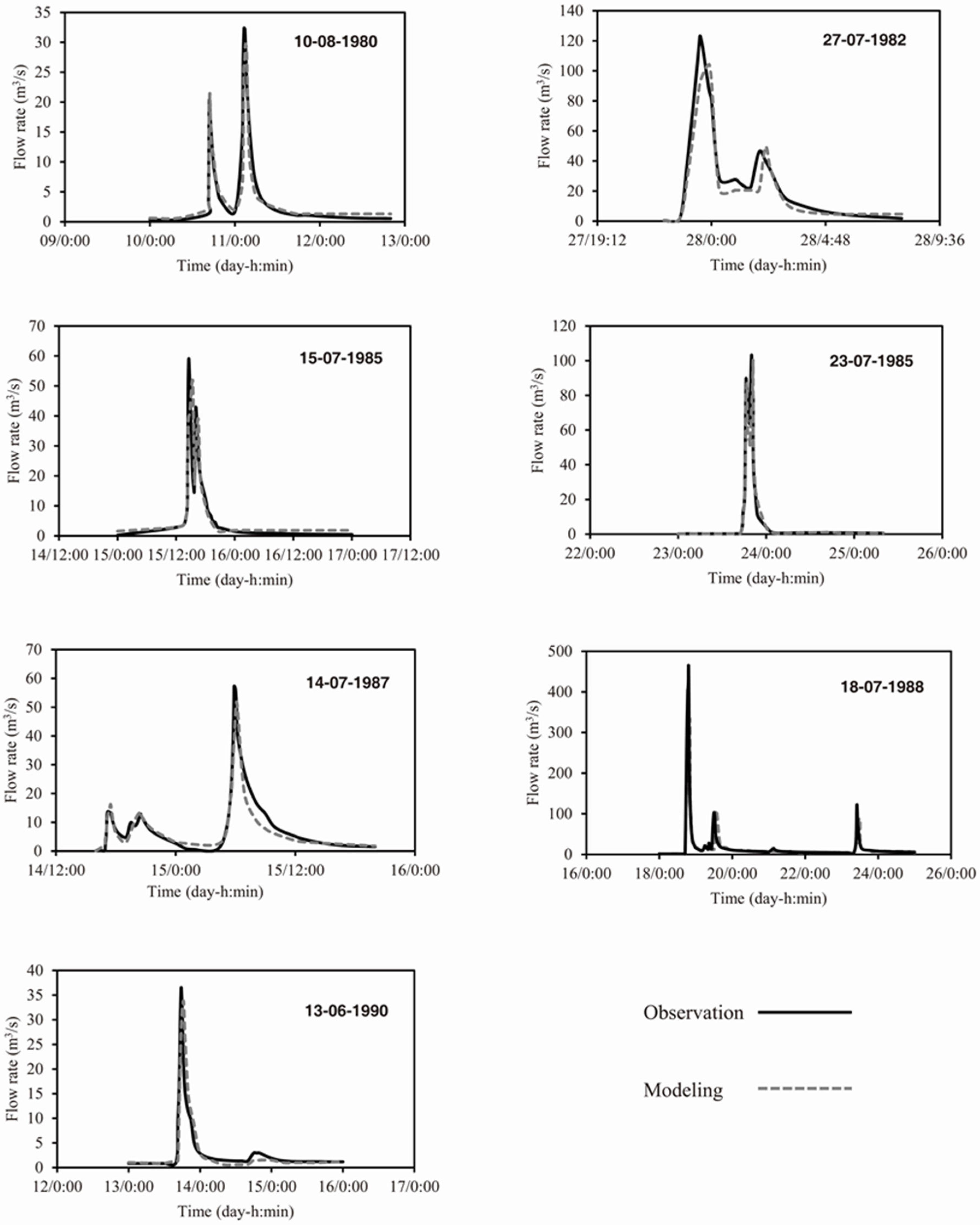
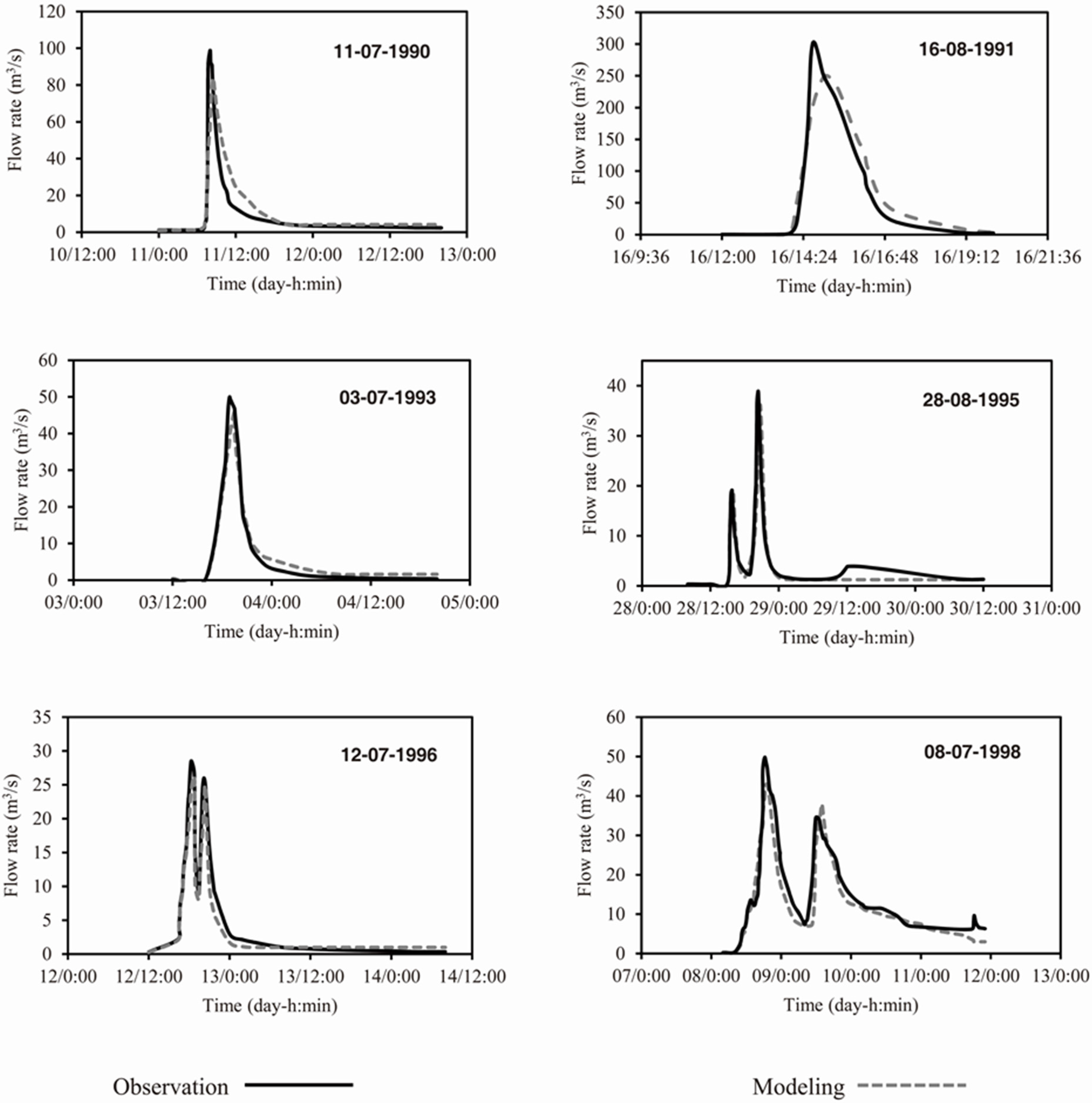
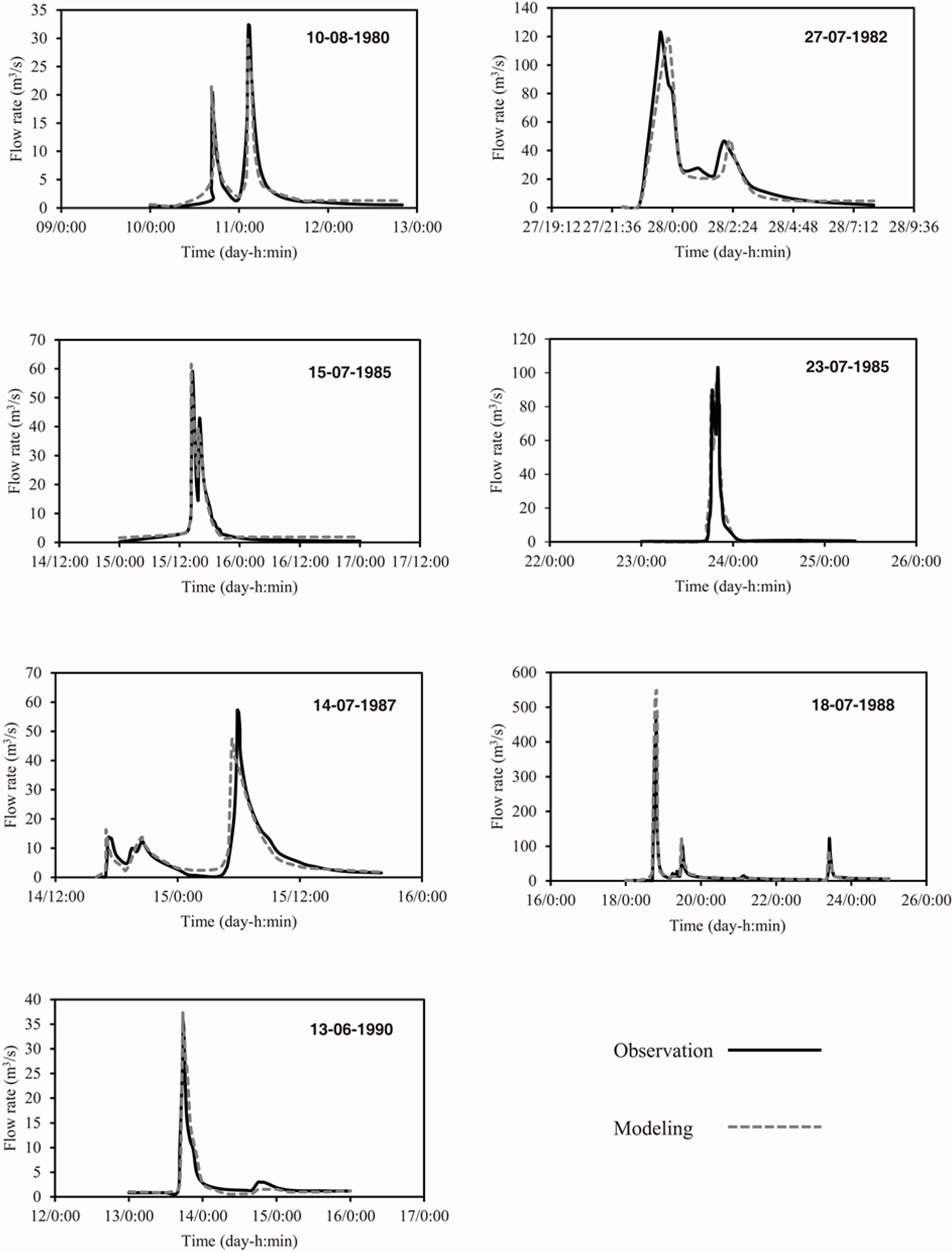
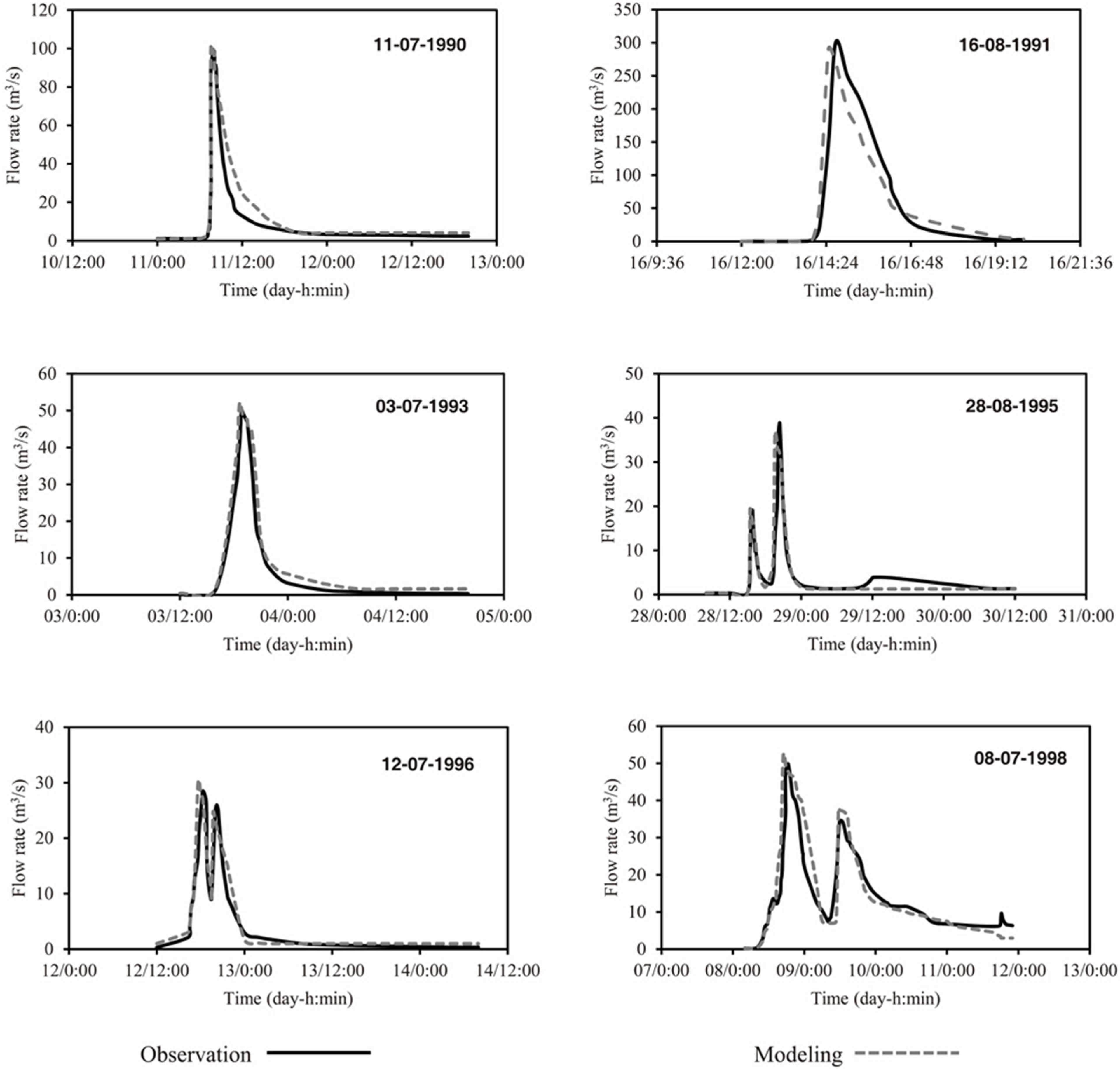
Table 7 and Table 8 list the modeling results of the flood volume, peak discharge, their relative errors with respect to the observation data, the difference between the modeled and the observed time of peak appearance, and the Nash efficiency coefficients for the two modeling schemes. Figure 3, Figure 4, Figure 5 and Figure 6 show the modeling and observed variation in the flow rate over time.

Table 7. The Modeling Results of Scheme I.

Recorded Events	Qs	Q0	REv	qs	q0	REp	∆T	DC
	104 m3	104 m3	%	m3/s	m3/s	%	min
Events for Calibration
10 August 1980	58.2	67.2	−13.4	29.7	32.4	−8.3	24	0.86
27 July 1982	71.7	87.9	−18.5	104.3	123	−15.2	22	0.87
15 July 1985	82.2	94.3	−12.8	51.4	59.1	−13.1	48	0.74
23 July 1985	79.9	92.8	−13.9	98.9	103	−3.9	25	0.92
14 July 1987	60.6	74.8	−18.9	51.8	57.2	−9.3	15	0.91
18 July 1988	579.5	933.2	−37.9	333.7	461	−27.6	45	0.84
13 June 1990	60.8	67.1	9.6	33.6	36	6.5	54	0.79
Events for Prediction
11 July 1990	128.7	118.8	8.3	83.6	98.8	−15.4	30	0.77
16 August 1991	177.5	169.7	4.6	248.1	300	−17.3	26	0.89
3 July 1993	43.19	47.5	−9.3	45.7	50	−8.5	34	0.93
28 August 1995	51.9	61.5	−15.6	36.1	38.9	−7.2	23	0.79
12 July 1996	48.8	56.1	−12.8	26.1	28.5	−8.5	28	0.93
08 July 1998	332.7	437.2	−23.9	42.9	49.8	−13.8	35	0.87

Table 7. The Modeling Results of Scheme I.

Recorded Events	Qs	Q0	REv	qs	q0	REp	∆T	DC
	104 m3	104 m3	%	m3/s	m3/s	%	min
Events for Calibration
10 August 1980	58.2	67.2	−13.4	29.7	32.4	−8.3	24	0.86
27 July 1982	71.7	87.9	−18.5	104.3	123	−15.2	22	0.87
15 July 1985	82.2	94.3	−12.8	51.4	59.1	−13.1	48	0.74
23 July 1985	79.9	92.8	−13.9	98.9	103	−3.9	25	0.92
14 July 1987	60.6	74.8	−18.9	51.8	57.2	−9.3	15	0.91
18 July 1988	579.5	933.2	−37.9	333.7	461	−27.6	45	0.84
13 June 1990	60.8	67.1	9.6	33.6	36	6.5	54	0.79
Events for Prediction
11 July 1990	128.7	118.8	8.3	83.6	98.8	−15.4	30	0.77
16 August 1991	177.5	169.7	4.6	248.1	300	−17.3	26	0.89
3 July 1993	43.19	47.5	−9.3	45.7	50	−8.5	34	0.93
28 August 1995	51.9	61.5	−15.6	36.1	38.9	−7.2	23	0.79
12 July 1996	48.8	56.1	−12.8	26.1	28.5	−8.5	28	0.93
08 July 1998	332.7	437.2	−23.9	42.9	49.8	−13.8	35	0.87

Table 8. The Modeling Results of Scheme II.

Recorded Events	Qs	Q0	REv	qs	q0	REp	∆T	DC
	104 m3	104 m3	%	m3/s	m3/s	%	min
Events for Calibration
10 August 1980	72.9	67.2	8.6	27.7	32.4	−14.3	−73	0.81
27 July 1982	81.3	87.9	−7.5	118.6	123	−3.5	18	0.86
15 July 1985	102.7	94.3	8.9	60.9	59.1	3.2	−15	0.71
23 July 1985	100.4	92.8	8.2	93.4	103	−9.3	−25	0.81
14 July 1987	67.5	74.8	−9.7	46.7	57.2	−18.2	−65	0.76
18 July 1988	1152.4	933.2	23.5	547.2	461	18.7	−35	0.71
13 June 1990	73.4	67.1	9.4	37.1	36	3.2	−15	0.88
Events for Prediction
11 July 1990	129.5	118. 9	8.9	101.6	98.8	2.8	−25	0.93
16 August 1991	150	169.7	−11.6	290.4	300	−3.2	−12	0.78
3 July 1993	51.4	47.5	8.2	52.5	50	4.3	−15	0.94
28 August 1995	56.1	61.6	−8.9	36.8	38.9	−5.5	−48	0.71
12 July 1996	61.9	56.1	10.6	30.6	28.5	7.3	−36	0.77
8 July 1998	529.9	437.2	21.2	52.4	49.8	5.3	−96	0.84

Table 8. The Modeling Results of Scheme II.

Recorded Events	Qs	Q0	REv	qs	q0	REp	∆T	DC
	104 m3	104 m3	%	m3/s	m3/s	%	min
Events for Calibration
10 August 1980	72.9	67.2	8.6	27.7	32.4	−14.3	−73	0.81
27 July 1982	81.3	87.9	−7.5	118.6	123	−3.5	18	0.86
15 July 1985	102.7	94.3	8.9	60.9	59.1	3.2	−15	0.71
23 July 1985	100.4	92.8	8.2	93.4	103	−9.3	−25	0.81
14 July 1987	67.5	74.8	−9.7	46.7	57.2	−18.2	−65	0.76
18 July 1988	1152.4	933.2	23.5	547.2	461	18.7	−35	0.71
13 June 1990	73.4	67.1	9.4	37.1	36	3.2	−15	0.88
Events for Prediction
11 July 1990	129.5	118. 9	8.9	101.6	98.8	2.8	−25	0.93
16 August 1991	150	169.7	−11.6	290.4	300	−3.2	−12	0.78
3 July 1993	51.4	47.5	8.2	52.5	50	4.3	−15	0.94
28 August 1995	56.1	61.6	−8.9	36.8	38.9	−5.5	−48	0.71
12 July 1996	61.9	56.1	10.6	30.6	28.5	7.3	−36	0.77
8 July 1998	529.9	437.2	21.2	52.4	49.8	5.3	−96	0.84

In the modeling, the parameters f_c and N showed a high sensitivity in Scheme I, while the CN showed a high sensitivity in Scheme II. Meanwhile, the Muskingum parameter K showed a high sensitivity in both schemes. These results demonstrate that the soil types, land use, basin topography and the river length play a major role in the flood run-off processes.

5.1. The Runoff-Volume Models

Schemes I and II employ the Initial and Constant-rate model and the SCS-CN model, respectively, to simulate runoff generation. According to the result of the flood volume relative error, RE_v, it can be seen that the error of Scheme I is relatively small for the four flood events, 13 June 1990, 11 July 1990, 16 August 1991, and 3 July 1993, with absolute values less than 10%, but the error increases significantly for the events of 27 July 1982, 14 July 1987, 28 July 1995, and 08 July 1998, with absolute values greater than 15%. However, the error of Scheme II has a small variation and a relatively small average absolute value for most of these events.

This can be explained by the following: due to the semi-arid and sub-humid attributes, the flood runoff is dominated by infiltration-excess under the condition of short but intensive rainfall, or by combined infiltration- and saturation-excess under the condition of long-lasting rainfall of various intensities. In Figure 3, Figure 4, Figure 5 and Figure 6, it can be seen that the floods on 13 June 1990, 11 July 1990 and 3 July 1993 were caused by rainfall of short duration, while the flood on 16 August 1991 was caused by rainfall with a strong intensity. The relative error of the flood volume of these events in Scheme I is relatively small and shows that the Initial and Constant-rate model is effective for modeling the infiltration-excess runoff. However, the increase in the error on 27 July 1982, 14 July 1987, 28 July 1995 and 8 July 1998 indicates that there was additional saturation-excess runoff, a fact that can been seen in Figure 3, Figure 4, Figure 5 and Figure 6, which shows that the four events had a long, continuous duration. Although the SCS-CN model in Scheme II demonstrated a better performance for runoff volume prediction, it needs to be pointed out that the SCS-CN is an empirical model, which does not consider extreme situations.

Figure 3. Flow Rate vs Time, Scheme I Calibration.

Figure 3. Flow Rate vs Time, Scheme I Calibration.

5.2. The Direct-Runoff and the Routing Models

Schemes I and II employ the Kinematic-wave model and the SCS-UH model, respectively, to simulate direct runoff. However, both schemes use the Muskingum model to simulate the routing (channel flow). For the floods on 15 July 1985, 13 June 1990, 11 July 1990, 16 August 1991 and 3 July 1993, which were short in duration and strong in intensity, as shown in Figure 3, Figure 4, Figure 5 and Figure 6, the difference between the predicted and observed (ΔT) peak time was within the range of 26–54 min in Scheme I compared with 15–25 min in Scheme II. For the floods on 10 August 1980, 14 July 1987, 28 August 1995 and 8 July 1998, which had long durations, the difference was within the range of 15–35 min using Scheme I and 48–96 min using Scheme II. The results show that the SCS-UH model of Scheme II is suitable for the situations of infiltration-excess, while the Kinematic-wave model of Scheme I is suitable for the situations of infiltration- and saturation-excess for semi-arid and sub-humid environmental conditions.

Figure 4. Flow Rate vs Time, Scheme I Prediction.

Figure 4. Flow Rate vs Time, Scheme I Prediction.

Figure 5. Flow rate vs time, scheme II calibration.

Figure 5. Flow rate vs time, scheme II calibration.

Figure 6. Flow Rate vs Time, Scheme II Prediction.

Figure 6. Flow Rate vs Time, Scheme II Prediction.

5.3. The Overall Comparison of the Two Modeling Schemes

From the modeling results shown in Table 7 and Table 8, it can be seen that 84.6% of the flood volume predictions of Scheme I had relative errors with absolute values less than 20%, while 92.3% of the predictions of Scheme II had relative errors less than 20%. For the flood peak discharge, 84.6% of the predictions of Scheme I had relative errors with absolute values less than 20%, while 100% of the predictions of Scheme II had relative errors with absolute values less than 20%. Meanwhile, the DCs were higher than 0.7 for all prediction cases. The results show that both schemes are viable to describe the flood-runoff processes in the Jianghe area. Overall, the average absolute values of the four performance indicator parameters in Scheme I are RE_v = 15.34, RE_p = 11.89, ΔT = 31.46 and DC = 0.85, compared with RE_v = 9.67, RE_p = 7.6, ΔT = 36.77 and DC = 0.8 in Scheme II. Overall, Scheme II performed better than Scheme I in the case study of the Janghe watershed.

6. Conclusions

This paper presents a case study of the modeling of the rainfall-runoff processes in a typical semi-arid and sub-humid region in northern China. Two schemes using the modeling tool HEC-HMS were investigated for the suitability and accuracy of the sub-component models provided. The proposed hydrological model is based on the hydrological characteristics, geo-topography, soil type and land use in the area. The models and predictions were validated and compared using observation data. The following four conclusions can be drawn from the study:

• The HEC-HMS is a suitable tool for modeling the rainfall-runoff processes in the Jianghe watershed, which is located in a typical region of semi-arid and sub-humid climate in northern China.
• The SCS-CN model performed better than the initial and constant-rate model in the estimation of runoff generation.
• The kinematic wave model demonstrated a relatively good result for the prediction of the flood peak time for situations of long-lasting rainfall duration with varied intensity, while the SCS-UH model demonstrated a relatively good result for situations with short rainfall duration but high intensity.
• An appropriate combination of the volume generation model and the direct runoff model is capable of producing reliable modeling estimates using the HEC-HMS for various applications. In general, Scheme II can be used for semi-arid and sub-humid environmental conditions.