The Probability Density Evolution Method for Flood Frequency Analysis: A Case Study of the Nen River in China

Abstract

A new approach for flood frequency analysis based on the probability density evolution method (PDEM) is proposed. It can avoid the problem of linear limitation for flood frequency analysis in a parametric method and avoid the complex process for choosing the kernel function and window width in the nonparametric method. Based on the annual maximum peak discharge (AMPD) in 54 years from the Dalai hydrologic station which is located on the downstream of Nen River in Heilongjiang Province of China, a joint probability density function (PDF) model about AMPD is built by the PDEM. Then, the numerical simulation results of the joint PDF model are given by adopting the one-sided difference scheme which has the property of direction self-adaptive. After that, according to the relationship between the marginal function and joint PDF, the PDF of AMPD can be obtained. Finally, the PDF is integrated and the frequency curve could be achieved. The results indicate that the flood frequency curve obtained by the PDEM has a better agreement with the empirical frequency than that of the parametric method widely used at present. The method based on PDEM is an effective way for hydrologic frequency analysis.

1. Introduction

The target of flood frequency analysis is to derive the probability distribution function (PDF) of annual maximum peak discharge (AMPD) according to the measured data. Then, the magnitude of a flood for a given return period can be estimated as the design basis of flood sluicing buildings, bridges, culverts, and other flood control projects[1,2]. Flood frequency analysis provides not only design basis for water conservancy projects which are going to be built, but also a calculation foundation for risk analysis and systematic use of water resources for those that have been built. Hence, flood frequency analysis is of great importance in hydraulic engineering. There have been numerous studies about it and the methods for flood frequency analysis can be divided into parametric method and nonparametric method, generally.

The parametric method for flood frequency analysis mainly includes two steps: (1) select an appropriate parent distribution for the measured data and, (2) estimate the parameters for the selected distribution. In regard to parent distribution selection, the Monte Carlo Bayesian method for a comprehensive study on computing the expected probability distribution was introduced by Kuczera [3]. A variety of mathematic test methods in flood parent distribution selection were adopted by Kite et al. [4,5,6,7,8]. Besides, the probability plot correlation coefficient (PPCC) test which was a powerful and easy-to-use goodness of fit test in completing samples for the composite hypothesis of normality was proposed by Filliben [9]. Thereafter, the PPCC test was extended for studying kinds of probability distribution types [10,11,12]. With respect to the parameter estimation research for the selected parent distribution, several methods have been extensively used, such as method of moments (MOM), method of maximum likelihood (ML), and curve-fitting method. The MOM, which includes the conventional moments [13], the linear moments (L-moments) [14,15,16,17,18], and the probability-weighted moments (PWM) [19,20,21,22,23,24,25,26,27,28], is the oldest way of deriving point estimators. The method of ML can give the most likely values of the parameters for a given distribution. It was adopted in estimating parameters for various distribution types [29,30] and different situations [31]. Moreover, El Adlouni, S. et al. [32] developed the generalized ML estimators for the nonstationary generalized extreme value model by incorporating the covariates into parameters. As to the curve-fitting method, it can be divided into two main categories, one is fitting the empirical frequency curve to the best by visual observation, the other is optimal curve-fitting method. Due to the characteristics of flexibility and easy manipulation, the curve-fitting method by visual observation is extensively applied in practical flood frequency analysis in China. However, the weakness of this method is prominent that different results may be obtained by different persons at different time. Obviously, it is not an objective method [33]. Thus, many researchers paid attention to the optimal curve-fitting method [34,35,36]. From the above studies, it can be seen that much work has been conducted on both steps of the parametric method. However, there still exists one problem in the parametric method because it is based on an assumption that the data in a given system obeys a certain distribution. It is regrettable that the limited distribution types cannot always satisfy all kinds of practice. Hence, there is the so-called linear limitation problem in parametric method. When the assumed parent distribution does not agree with the fact, the precision of corresponding calculation results cannot be guaranteed.

For the linear limitation problem in the parametric method, Tung [37] proposed the application of the nonparametric method in hydraulic frequency analysis in 1981 for the first time. The nonparametric method can solve the linear limitation problem for the reason that the process of parent distribution assumption is avoided. Therefore, it was employed and emphasized in this field gradually [38,39,40,41,42,43,44]. Nevertheless, the defect of the nonparametric method is also evident that there is no specific criteria about how to select a better kernel function and window width in different situations. Because of this, it is difficult to take use of the nonparametric method in practice [45]. Thereby, a method which does not need to choose kernel function and window width, meanwhile the assumption of parent distribution can be avoided, is necessarily demanded.

The probability density evolution method (PDEM) which has no need of assuming a parent distribution in flood frequency analysis takes the probability conservation principle, which means that the law of probability conservation exists during the state evolution process for a conservative stochastic system, as the theoretical foundation. The basic idea of using PDEM in flood frequency analysis is different from the nonparametric method. Therefore, the process of choosing kernel function as well as window width is avoided, and the PDEM is adopted for flood frequency analysis in this paper. Firstly, the joint PDF model about AMPD is established through PDEM. And then, by means of numerical method, the model is able to be solved and the probability density value as well as the probability distribution value of AMPD can be obtained. Finally, the frequency curve will be achieved.

This paper is organized as follows: in Section 2, the basic idea of the PDEM is introduced. In Section 3, a model about the joint PDF of AMPD is derived based on the PDEM. The solution method about the model and frequency values calculation of AMPD are suggested. Also presented in this section is the robustness study about the proposed method by statistical experiment research (Monte-Carlo method). An example and discussion will be given in Section 4, while the last section contains a brief summary of the results.

2. Probability Density Evolution Method

Due to the coupling effect between nonlinear and stochastic, the accurate prediction of nonlinear response for practical engineering structure is difficult to implement. In the light of this, Li and Chen [46,47] developed an in-depth study on the principle of probability conservation and derived the PDEM by the combination of state space description for principle of probability conservation and different physical equations, such as the classical Liouville Equation, Fokker Planck Kolmogorov (FPK) Equation, and Dostupov–Pugachev (D–P) Equation. The PDF of structure response containing the whole stochastic factors in the dynamic system can be acquired through the numerical solution of probability density evolution equation. Thus, in recent years, a systematic research of the PDEM has been made in stochastic response analysis of multi-dimensional linear and nonlinear structure systems, calculation of dynamic reliability and system reliability, as well as control aspects based on reliability. The basic idea of PDEM is briefly introduced as follows [48,49].

Suppose that an m-dimension virtual stochastic process can be described as:

$$\mathbf{X}=\mathrm{\Phi }(\mathbf{\Theta },\text{τ}),{\mathit{X}}_l={\mathrm{\Phi }}_l(\mathbf{\Theta },\text{τ})$$

(1)

where, X is the state vector, Φ represents the mapping relationship between X and Θ, τ. Θ is random vector, τ is virtual time. X_l and Φ_l are the l-th component of X and Θ, respectively, l = 1, 2,…, m, m is an integer.

According to the probability compatibility condition, when {Θ = θ}, the expression about X_l(τ) can be obtained:

$${\displaystyle \underset{-\infty }{\overset{\infty }{\int }}{P}_{{\mathit{X}}_{\mathit{l}}|\mathbf{\Theta }}(x,\text{τ}|\text{θ})\text{d}}x=1$$

(2)

where $P_{{\mathit{X}}_{\mathit{l}}|\mathbf{\Theta }}(x,\text{τ}|\text{θ})$ is the conditional PDF of X_l(τ) at {Θ = θ}.

From Equation (1), it is known that X_l = H_l(θ,τ) when {Θ = θ}, namely, the probability of X_l = H_l(θ,τ) equals 1 when {Θ = θ}. Therefore, the probability of X_l ≠ H_l(θ,τ) must be 0. Combining above analysis with Equation (2) yields:

$$P_{{\mathit{X}}_{\mathit{l}}|\mathbf{\Theta }}(x,\text{τ}|\text{θ})=\{\begin{array}{l}0,x\ne H_l(\text{θ,τ})\\ \infty ,x=H_l(\text{θ,τ})\end{array}$$

(3)

Equations (2) and (3) fit the definition of Dirac Function. Hence, they can be comprehensively expressed as:

$$P_{{\mathit{X}}_{\mathit{l}}|\mathbf{\Theta }}(x,\text{τ}|\text{θ})=\text{δ}(x-H_l(\text{θ,τ}))$$

(4)

where δ(·) is the Dirac’s Function.

According to the conditional probability formula, the joint PDF of stochastic variable (X_l(τ), Θ) which is denoted as $P_{{\mathit{X}}_l\mathbf{\Theta }}(x,\text{θ,τ})$ can be derived from Equation (4):

$$P_{{\mathit{X}}_{\mathit{l}}\mathbf{\Theta }}(x,\text{θ,τ})=P_{{\mathit{X}}_{\mathit{l}}|\mathbf{\Theta }}(x,\text{τ}|\text{θ})P_{\mathbf{\Theta }}(\text{θ})=\text{δ}(x-H_l(\text{θ,τ}))P_{\mathbf{\Theta }}(\text{θ})$$

(5)

where P_Θ(θ) is the PDF of Θ.

Differentiating Equation (5) on both sides with regard to τ, and using the derivation rule of compound function will yield:

$$\frac{\partial P_{{\mathit{X}}_{\mathit{l}}\mathbf{\Theta }}(x,\text{θ,τ})}{\partial \text{τ}}=P_{\mathbf{\Theta }}(\text{θ})\frac{\partial \left[\text{δ}(x-H_l(\text{θ,τ}))\right]}{\partial \text{τ}}=P_{\mathbf{\Theta }}(\text{θ}){\left[\frac{\partial \left[\text{δ}(y)\right]}{\partial y}\right]}_{y=x-H_l(\theta \text{, }\tau )}\frac{\partial y}{\partial \text{τ}}$$

(6)

Because both θ and τ are fixed values in the differential process of compound function, the partial derivative of y = x − H_l(θ,τ) is dy = dx. Therefore, substitute ∂y in Equation (6) with ∂x. Then, Equation (6) can be rewritten as follow:

$$\begin{array}{l}\frac{\partial P_{{\mathit{X}}_{\mathit{l}}\mathbf{\Theta }}(x,\text{θ,τ})}{\partial \text{τ}}=-P_{\mathbf{\Theta }}(\text{θ})\frac{\partial \left[\text{δ}(x-H_l(\text{θ,τ}))\right]}{\partial x}\frac{\partial H_l(\text{θ,τ})}{\partial \text{τ}}\\ \text{ =}-\frac{\partial \left[\text{δ}(x-H_l(\text{θ,τ}))P_{\mathbf{\Theta }}(\text{θ})\right]}{\partial x}\frac{\partial H_l(\text{θ,τ})}{\partial \text{τ}}\\ =-{\dot{H}}_l(\text{θ,}t)\frac{\partial P_{{\mathit{X}}_{\mathit{l}}\mathbf{\Theta }}(x,\text{θ},t)}{\partial x}\end{array}$$

(7)

that is:

$$\frac{\partial P_{{\mathit{X}}_{\mathit{l}}\mathbf{\Theta }}(x,\text{θ,τ})}{\partial \text{τ}}+{\dot{H}}_l(\text{θ,τ})\frac{\partial P_{{\mathit{X}}_{\mathit{l}}\mathbf{\Theta }}(x,\text{θ,τ})}{\partial x}=0$$

(8)

Equation (8) is the probability density evolution equation, and the corresponding initial condition can be conveniently obtained from Equation (5):

$$P_{{\mathit{X}}_{\mathit{l}}\mathbf{\Theta }}(x,\text{θ,τ}){|}_{\text{τ}=0}=\text{δ}(x-x_{0,l})P_{\mathbf{\Theta }}(\text{θ})$$

(9)

where x_0,l is the l-th component of x₀.

The boundary condition of Equation (8) reads as:

$$P_{{\mathit{X}}_{\mathit{l}}\mathbf{\Theta }}(x,\text{θ,τ}){|}_{x\to \pm \infty }=0$$

(10)

By means of numerical difference method, the probability density evolution equation can be solved based on Equations (9) and (10). Thus, the joint PDF $P_{{\mathit{X}}_{\mathit{l}}\mathbf{\Theta }}(x,\text{θ,τ})$ is obtained. In accordance with the relationship between the marginal function and joint PDF, the PDF $P_{{\mathit{X}}_{\mathit{l}}}(x,\text{τ})$ can be acquired:

$$P_{{\mathit{X}}_{\mathit{l}}}(x,\text{τ})={\displaystyle {\int }_{{\Omega }_{\text{θ}}}{P}_{{\mathit{X}}_{\mathit{l}}\mathbf{\Theta }}(x,\text{θ,τ})d}\text{θ}$$

(11)

where Ω_θ is the distribution domain of Θ.

3. The Flood Frequency Analysis Method Based on PDEM

3.1. The Joint PDF Model for Peak Discharge

In flood frequency analysis, the sample of AMPD, which is composed of measured data from the hydrologic stations for years, can be denoted as Z = (z₁, z₂, z₃,…, z_n), here n is the total number of data in the sample. With consideration of the stochastic characteristic of hydrologic variables, the AMPD can be expressed by a one-dimension static stochastic process Y (y).

Construct a one-dimension stochastic process:

$$\mathit{X}(t)=H(\mathit{Z},t)=Y(y)\cdot t$$

(12)

then

$$Y(y)=\mathit{X}(t){|}_{t=1}=H(\mathit{Z},t){|}_{t=1}$$

(13)

where, X(t) is the state vector of parent peak discharge. H represents the mapping relationship between X and Z, t. Z is the random vector consisting of peak discharge measurement of data. t is time.

It can be seen from Equation (13) that the PDF of AMPD can be obtained through the derivation of PDF for one-dimension stochastic process X(t) at t = 1.

Comparing Equation (12) with Equation (1), it is found that both forms of them are consistent. Therefore, a joint probability density evolution equation of (X, Z) corresponding to Equation (8) can be obtained as follows:

$$\frac{\partial P_{\mathit{X}\mathit{Z}}(x,z,t)}{\partial t}+\dot{H}(z\text{,}t)\frac{\partial P_{\mathit{X}\mathit{Z}}(x,z,t)}{\partial x}=0$$

(14)

where P_XZ(x,z,t) is the joint PDF of (X, Z).

Discretize z and bring the measured data in Equation (14). Then, the joint PDF model of peak discharge can be acquired:

$$\frac{\partial P_{\mathit{X}\mathit{Z}}(x,z_j,t)}{\partial t}+\dot{H}(z_j\text{,}t)\frac{\partial P_{\mathit{X}\mathit{Z}}(x,z_j,t)}{\partial x}=0(j=1,2,\cdots n,0\le t\le 1)$$

(15)

Considering that the acquisition of the measured data for AMPD is an independent process; therefore; when there is no any other additional information; the probability of the measured data for AMPD which is denoted as P_Z(z_j) can be described as:

$$P_{\mathit{Z}}(z_j)=\frac{1}{n}$$

(16)

Taking into account Equations (9) and (16), the initial condition of Equation (15) can be written as:

$$P_{\mathit{X}\mathit{Z}}(x,z,t){|}_{t=0}=\text{δ}(x-x_0)P_{\mathit{Z}}(z_j)=\text{δ}(x-x_0)\frac{1}{n}$$

(17)

where x₀ is the initial value of AMPD.

According to reference [50], the system state H(z,t) can be expressed as:

$$H(z,t)=z\sin (2.5\text{π}t)$$

(18)

In this way, the discrete form of velocity function in Equation (15) is taken as follows:

$$\dot{H}(z_j,t)=z_j\cos (2.5\text{π}t)\cdot 2.5\text{π}$$

(19)

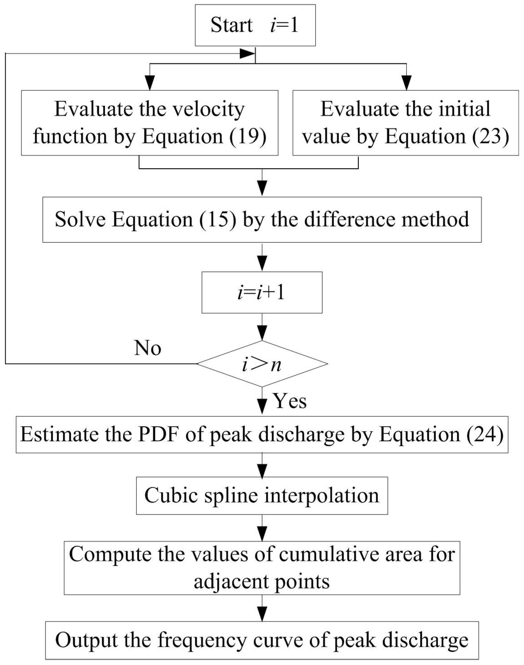
3.2. Model Solution and Frequency Values Calculation of Peak Discharge

Equation (15) is the one-dimension variable coefficients convection equation, which can be solved by many finite difference methods. According to calculation experience, a fairly satisfactory calculation precision will be achieved by adopting the one-sided difference scheme. Considering that the sign of the velocity function may change between positive and negative with the variation of time t, in this paper, the one-sided difference scheme possessing the characteristic of direction adaptive is selected to discretize Equation (15) as follows:

$$P_{j,m}=(1-\left|h_m{r}_L\right|)p_{j,m-1}+\frac{1}{2}(h_m{r}_L+\left|h_m{r}_L\right|)p_{j-1,m-1}-\frac{1}{2}(h_m{r}_L-\left|h_m{r}_L\right|)p_{j+1,m-1}$$

(20)

$$h_m=\frac{1}{2}(\dot{H}({\text{z}}_j\text{,}{t}_{m-1})+\dot{H}({\text{z}}_j\text{,}{t}_m))$$

(21)

where P_j,m denotes the discrete form of joint PDF for XZ and is short for P_XZ(x_i,z_j,t_m), in which x_i = iΔx (i = 0, ±1, ±2,…), t_m = mΔt(m = 0,1, 2,…). x_i and t_m are the discrete values of calculation interval for time axis and space axis, respectively. Δx and Δt are the space step and time step, respectively, r_L is the ratio of Δt to Δx.

In order to ensure the convergence of the calculation results, the Courant–Friedrichs–Lewy condition for the difference scheme of Equation (20) is needed:

$$\left|h_m{r}_L\right|\le 1,\mathbf{\forall }m=0,1,2\cdots$$

(22)

After establishing the joint PDF model of peak discharge and selecting a suitable difference scheme, the calculation of flood frequency based on PDEM can be described as follows:

(1) Determine space step Δx and time step Δt for evaluating the velocity function and initial condition. First of all, select a suitable Δx and Δt according to Equation (22) by trial method. Secondly, denote the discrete points of time axis in the domain [0, 1] as t_m. Thus, the velocity function can be calculated through Equation (19). Likewise, denote the discrete points of space axis in the corresponding domain as x_i. After that, the discrete form of Equation (17) can be given as:

$$P_{XZ}(x_i,z_j,t_0)=\{\begin{array}{c}\frac{1}{\left|\mathrm{\Delta }x\right|n}\\ 0\end{array}\begin{array}{c}i=0\\ \begin{array}{}\\ i\ne 0\end{array}\end{array}$$

(23)

(2) Solve Equation (15) by employing the difference scheme of Equation (20). Then, the discrete value of joint PDF P_XZ(x_i,z_j,t_m) at t_m = 1 can be acquired.

(3) Conduct the numerical integration with respect to z_j according to Equation (11). Thereby, the discrete PDF will be written as:

$$P_Y(y)=P_X(x,t){|}_{t=1}={\displaystyle \sum _{j=1}^n{P}_{XZ}(x_i,z_j,t)}{|}_{t=1}$$

(24)

(4) Calculate the frequency values of peak discharge through the discrete PDF. Firstly, in order to get a better calculation precision for the flood frequency, the cubic spline interpolation on the PDF of peak discharge calculated by Equation (24) is implemented. Secondly, the trapezoid method is adopted to calculate the area value between the adjacent points on the curve of peak discharge PDF which has already been interpolated. Then, the values of cumulative area with descending order of peak discharge are computed. Finally, the flood frequency can be obtained.

The flowchart of the flood frequency calculation based on the PDEM is depicted in Figure 1.

Figure 1. Flowchart of the flood frequency calculation based on the PDEM.

Figure 1. Flowchart of the flood frequency calculation based on the PDEM.

3.3. The Robustness Study for PDEM

In order to analyze the robustness of the proposed method, the statistical experiment research (Monte–Carlo method) is adopted. Since the measured hydrological data of natural rivers is relatively short, usually less than 60 years, hence, the statistical experiment research with small samples has actual hydrological significance. In order to evaluate the robustness of PDEM, two commonly used parent distribution types for hydrology in this statistical test are taken to analyze and calculate two groups of samples and four parent parameters, with a total of 32 programs. The specific steps for the robustness study are as follows:

• Give the parent parameters of statistical distribution and assume their distribution types, then extract m group of sample series with the length of n from every parent distribution.
• Calculate the design value of design frequency with PDEM.
• Analyze various types of error of design value and study their robustness.

The specific plan is as follows:

(1)

The parent distribution: Pearson Type III, Log Normal.

(2)

Estimation method: the probability density evolution method (PDEM).

(3)

Sample size: n = 30, n = 50.

(4)

Design frequency: p₁ = 0.02, p₂ = 0.01.

(5)

Parent parameters: As seen in Table 1.

(6)

Sampling times: m = 50.

(7)

Evaluation criteria: Relative mean square (RMS) error and relative error of the mean design value (as shown in Equations (25) and (26)).

The relative RMS error is:

$$\text{δ=}\frac{\text{1}}{x_p}\sqrt{\frac{{\displaystyle \sum _{i=1}^m{({\stackrel{⌢}{x}}_{pi}-x_p)}^2}}{m}}\times 100\%$$

(25)

$$\text{ω}=\frac{1}{x_p}\left|\frac{1}{m}{\displaystyle \sum _{i=1}^m{\stackrel{⌢}{x}}_{pi}}\text{-}{x}_p\right|\times 100\%$$

(26)

The relative error of the mean design value is:

where, xp represents a true value of design frequency p whose distribution is known, ${\stackrel{⌢}{x}}_{pi}$ is the design value of estimated p.

Table 1. Parent parameters.

No.	Mean (EX)	Coefficient of Variation (Cv)	Coefficient of Skewness (Cs)
1	1000	1.0	2.5
2	1000	1	3
3	1000	2	4
4	1000	2.5	5

Table 1. Parent parameters.

No.	Mean (EX)	Coefficient of Variation (Cv)	Coefficient of Skewness (Cs)
1	1000	1.0	2.5
2	1000	1	3
3	1000	2	4
4	1000	2.5	5

The calculation results of 32 plans about statistical tests mentioned-above can be seen in Table 2 and Table 3. It can be found for both distribution of Log Normal and Pearson Type III, the relative error of the mean design value ω does not exceed 15%, and the relative RMS error δ of that is not greater than 40%. In addition, the corresponding design value of same design frequency calculated by different theoretical parent distribution is relatively close. It is demonstrated that the difference of theoretical population has little influence on the calculation results. Therefore, as an estimated method of design value, the PDEM is relatively robust.

Table 2. The results calculated by PDEM with theoretical population of Log Normal distribution.

No.	p	n	Parent Parameters	True Value	Mean Value of Design Value	δ	ω
1	0.02	30		3913.10	4022.49	26.45	2.80
2	0.01		Cv = 1	4899.40	4713.69	27.9	3.79
3	0.02	50	Cs = 2.5	3913.10	4161.22	24.19	6.34
4	0.01			4899.40	4442.61	28.92	9.32
5	0.02	30		3913.10	3685.51	34.58	5.82
6	0.01		Cv = 1	4899.40	4416.54	34.5	9.86
7	0.02	50	Cs = 3	3913.10	4262.01	27.46	8.92
8	0.01			4899.40	5169.09	29.37	5.50
9	0.02	30		6063.75	6468.00	29.21	6.67
10	0.01		Cv =2	8540.85	8944.98	36.21	4.73
11	0.02	50	Cs = 4	6063.75	6797.37	30.62	12.10
12	0.01			8540.85	7806.87	34.83	8.59
13	0.02	30		6698.42	7196.04	31.69	7.43
14	0.01		Cv = 2.5	9795.19	8829.59	36.55	9.86
15	0.02	50	Cs = 5	6698.42	7307.51	19.11	9.09
16	0.01			9795.19	10,340.84	29.9	5.57

Table 2. The results calculated by PDEM with theoretical population of Log Normal distribution.

No.	p	n	Parent Parameters	True Value	Mean Value of Design Value	δ	ω
1	0.02	30		3913.10	4022.49	26.45	2.80
2	0.01		Cv = 1	4899.40	4713.69	27.9	3.79
3	0.02	50	Cs = 2.5	3913.10	4161.22	24.19	6.34
4	0.01			4899.40	4442.61	28.92	9.32
5	0.02	30		3913.10	3685.51	34.58	5.82
6	0.01		Cv = 1	4899.40	4416.54	34.5	9.86
7	0.02	50	Cs = 3	3913.10	4262.01	27.46	8.92
8	0.01			4899.40	5169.09	29.37	5.50
9	0.02	30		6063.75	6468.00	29.21	6.67
10	0.01		Cv =2	8540.85	8944.98	36.21	4.73
11	0.02	50	Cs = 4	6063.75	6797.37	30.62	12.10
12	0.01			8540.85	7806.87	34.83	8.59
13	0.02	30		6698.42	7196.04	31.69	7.43
14	0.01		Cv = 2.5	9795.19	8829.59	36.55	9.86
15	0.02	50	Cs = 5	6698.42	7307.51	19.11	9.09
16	0.01			9795.19	10,340.84	29.9	5.57

Table 3. The results calculated by PDEM with theoretical population of Pearson Type III distribution.

No.	p	n	Parent Parameters	True Value	Mean Value of Design Value	δ	ω
17	0.02	30		4040	3926.20	17.74	2.82
18	0.01		Cv = 1	4850	4468.80	27.9	7.86
19	0.02	50	Cs = 2.5	4040	4076.80	17.71	0.91
20	0.01			4850	4645.50	25.58	4.22
21	0.02	30		4150	3967.60	29.5	4.40
22	0.01		Cv = 1	5050	4714.50	29.83	6.64
23	0.02	50	Cs = 3	4150	4372.20	21.08	5.35
24	0.01			5050	5118.10	24.99	1.35
25	0.02	30		7300	7045.80	16.75	3.48
26	0.01		Cv = 2	9100	8454.10	28.66	7.10
27	0.02	50	Cs = 4	7300	6910	24.95	5.34
28	0.01			9100	9001	33.44	1.09
29	0.02	30		8875	8135	23.3	8.34
30	0.01		Cv = 2.5	11,125	9593	24.43	13.77
31	0.02	50	Cs = 5	8875	8506	28.62	4.16
32	0.01			11,125	10,104	30.72	9.18

Table 3. The results calculated by PDEM with theoretical population of Pearson Type III distribution.

No.	p	n	Parent Parameters	True Value	Mean Value of Design Value	δ	ω
17	0.02	30		4040	3926.20	17.74	2.82
18	0.01		Cv = 1	4850	4468.80	27.9	7.86
19	0.02	50	Cs = 2.5	4040	4076.80	17.71	0.91
20	0.01			4850	4645.50	25.58	4.22
21	0.02	30		4150	3967.60	29.5	4.40
22	0.01		Cv = 1	5050	4714.50	29.83	6.64
23	0.02	50	Cs = 3	4150	4372.20	21.08	5.35
24	0.01			5050	5118.10	24.99	1.35
25	0.02	30		7300	7045.80	16.75	3.48
26	0.01		Cv = 2	9100	8454.10	28.66	7.10
27	0.02	50	Cs = 4	7300	6910	24.95	5.34
28	0.01			9100	9001	33.44	1.09
29	0.02	30		8875	8135	23.3	8.34
30	0.01		Cv = 2.5	11,125	9593	24.43	13.77
31	0.02	50	Cs = 5	8875	8506	28.62	4.16
32	0.01			11,125	10,104	30.72	9.18

4. Case sStudy

4.1. Study Area

In this study, flood frequency analysis is performed on the Nen River in Heilongjiang Province in Northeast China. The Nen River is the biggest tributary of the Songhua River, whose annual runoff and catchment are ranked third among all of the rivers in China. The area of the Nen River basin is approximately 297,000 km², and the full-length of its main stream is more than 1370 km. In addition, the climate characteristic of this basin is that winter is long and cold, while summer is short and rainy. About 82% annual precipitation comes from June to September. The Dalai hydrologic station is a central control station located at the downstream of the Nen River. According to the data of AMPD in Table 4, which covers 54 years measured data from Dalai hydrologic station, the PDF and the frequency of AMPD based on the PDEM are studied.

Table 4. The measured data of annual maximum peak discharge (AMPD) from Dalai hydrologic station.

Year	AMPD (m3/s)	Year	AMPD (m3/s)	Year	AMPD (m3/s)	Year	AMPD (m3/s)	Year	AMPD (m3/s)
1951	3760	1962	4090	1973	2410	1984	4250	1995	1610
1952	2100	1963	3470	1974	825	1985	2500	1996	3970
1953	4750	1964	1510	1975	1270	1986	3690	1997	2100
1954	1480	1965	2980	1976	1370	1987	1980	1998	16100
1955	3200	1966	2330	1977	1770	1988	5640	1999	1890
1956	6370	1967	1410	1978	899	1989	5280	2000	1380
1957	7790	1968	740	1979	588	1990	3950	2001	1160
1958	4570	1969	8810	1980	3110	1991	6370	2002	541
1959	2920	1970	1990	1981	2950	1992	2010	2003	4590
1960	5760	1971	1400	1982	1060	1993	5780	2004	2280
1961	3130	1972	1920	1983	3860	1994	1710	-	-

Table 4. The measured data of annual maximum peak discharge (AMPD) from Dalai hydrologic station.

Year	AMPD (m3/s)	Year	AMPD (m3/s)	Year	AMPD (m3/s)	Year	AMPD (m3/s)	Year	AMPD (m3/s)
1951	3760	1962	4090	1973	2410	1984	4250	1995	1610
1952	2100	1963	3470	1974	825	1985	2500	1996	3970
1953	4750	1964	1510	1975	1270	1986	3690	1997	2100
1954	1480	1965	2980	1976	1370	1987	1980	1998	16100
1955	3200	1966	2330	1977	1770	1988	5640	1999	1890
1956	6370	1967	1410	1978	899	1989	5280	2000	1380
1957	7790	1968	740	1979	588	1990	3950	2001	1160
1958	4570	1969	8810	1980	3110	1991	6370	2002	541
1959	2920	1970	1990	1981	2950	1992	2010	2003	4590
1960	5760	1971	1400	1982	1060	1993	5780	2004	2280
1961	3130	1972	1920	1983	3860	1994	1710	-	-

4.2. Data Analysis Method and Parameters Selection

To show the rationality of the calculation results based on PDEM, two groups of comparisons are conducted:

(1)

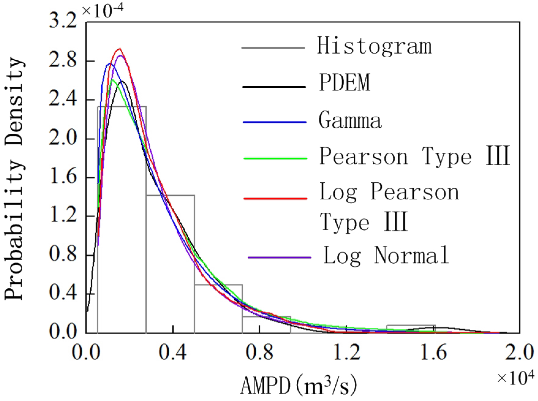
The comparison between frequency histogram and the PDF of peak discharge calculated by PDEM as well as parametric method.

(2)

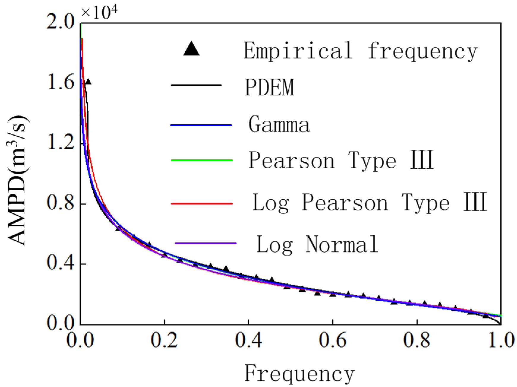
The comparison between empirical frequency and the frequency values of peak discharge calculated by PDEM as well as parametric method.

All the calculations in above comparisons are carried out based on the Matlab software. The interval number of frequency histogram in this study is evaluated by the following equation as mentioned in [51]:

$$k=1+{\log }_{2}n$$

(27)

where k is the interval number.

As to the empirical frequency, it is derived from the expectation equation wholly adopted in hydrological frequency analysis at present. Arrange the measured data in a descending order, as z₁, z₂,…, z_m,…, z_n. Then, the empirical frequency of peak discharge sample F_e(z_i) can be expressed as:

$$F_{\text{e}}\left(z_i\right)=\frac{m}{n+1}$$

(28)

The related parameters of the flood frequency analysis method used in this paper are given as follows: the time step Δt and the space step Δx are selected according to Equation (22) by trial method. When Δt equals to 0.0001 s and Δx equals to 19.95 m³/s, Equation (22) can be satisfied. Taking into account that the value of AMPD is greater than zero, the initial sample value x₀ can be selected between zero and the minimum value of measured data. From Table 4, it can be seen that the minimum value and the maximum value of AMPD are 541 m³/s and 16,100 m³/s, respectively. Hence, set x₀ = 50 m³/s, and the calculation interval of AMPD is selected ranging from 50 to 20,000 m³/s.

4.3. Results and Discussion

During the process of parent distribution selection in parametric method, three fitting methods including the chi-square test, the Kolmogorov–Smirnov test, and the Anderson–Darling test are employed to analyze six kinds of distribution types which are often used in hydrologic frequency analysis. The parameters of them are estimated by the method of ML, and the relevant results are listed in Table 5. The results of goodness of fit tests are summarized in Table 6. The calculation methods of statistic values for fit tests in Table 6 are introduced in reference [52]. It can be seen from Table 6 that the order of calculation results obtained by chi-square test are somewhat different with those obtained by the other two tests. However, the top four orders of distribution types, namely Log Pearson Type III distribution, Log Normal distribution, Gamma distribution, and Pearson Type III distribution are identical. Hence, the above four distribution types are selected for subsequent investigations.

Table 5. Estimated parameter values of different distribution types.

Distribution	Log Pearson Type III	Log Normal	Gamma	Weibull (3P)	Pearson Type III	Gumbell
Parameters	α = 59226	σ = 0.699 μ = 7.842	α =1.5753 β =2061.6	α = 1.114	α = 3.822	σ = 2017.500 μ = 2083.100
	β = 0.003			β = 2825.100	β = 11163
	γ = −163.820			γ = 532.690	γ = −670.590

Table 5. Estimated parameter values of different distribution types.

Distribution	Log Pearson Type III	Log Normal	Gamma	Weibull (3P)	Pearson Type III	Gumbell
Parameters	α = 59226	σ = 0.699 μ = 7.842	α =1.5753 β =2061.6	α = 1.114	α = 3.822	σ = 2017.500 μ = 2083.100
	β = 0.003			β = 2825.100	β = 11163
	γ = −163.820			γ = 532.690	γ = −670.590

Table 6. The results of goodness of fit tests.

Distribution	Kolmogorov Smirnov		Anderson Darling		Chi-Squared
	Statistic	Rank	Statistic	Rank	Statistic	Rank
Log Pearson Type III	0.059	1	0.151	1	2.011	3
Log Normal	0.060	2	0.153	2	1.999	2
Gamma	0.071	4	0.247	4	1.624	1
Weibull (3P)	0.079	5	0.310	5	2.957	5
Pearson Type III	0.067	3	0.185	3	2.039	4
Gumbell	0.082	6	0.379	6	3.313	6

Table 6. The results of goodness of fit tests.

Distribution	Kolmogorov Smirnov		Anderson Darling		Chi-Squared
	Statistic	Rank	Statistic	Rank	Statistic	Rank
Log Pearson Type III	0.059	1	0.151	1	2.011	3
Log Normal	0.060	2	0.153	2	1.999	2
Gamma	0.071	4	0.247	4	1.624	1
Weibull (3P)	0.079	5	0.310	5	2.957	5
Pearson Type III	0.067	3	0.185	3	2.039	4
Gumbell	0.082	6	0.379	6	3.313	6

According to the PDF expression of the selected distributions, the calculation results of PDF by the parametric method can be achieved as seen in Figure 2. In the same way, through the expression of PDF, the frequency values of peak discharge can also be obtained, as depicted in Figure 3.

Figure 2. Probability density curve of AMPD from Dalai hydrologic station.

Figure 2. Probability density curve of AMPD from Dalai hydrologic station.

Figure 3. Frequency curve of AMPD from Dalai hydrologic station.

Figure 3. Frequency curve of AMPD from Dalai hydrologic station.

It can be seen from Figure 2 that the trends of probability density curve for AMPD calculated by parametric method with four distributions are similar, but the right tail does not agree well with the frequency histogram. For the matching result calculated by PDEM, it has a better agreement with the frequency histogram, even the mutational parts on the right tail of the probability density curve are included. Hence, compared with the parametric method, taking use of PDEM can show the preferable effect on the distribution structure of PDF for AMPD. The reason for this is that PDEM is a kind of method which can be directly estimated through the sample data and does not need to assume a parent distribution. Moreover, it can also simulate different types of measured data, including data with multi-peak distribution, which is impossible to be realized by parametric method.

Figure 3 is the frequency curve of peak discharge calculated by PDEM and the parametric method. It is shown that both methods can fit well with the empirical frequency points at the middle of the frequency interval, however, at the two ends of the frequency interval, more points will be fitted by means of the PDEM instead of the parametric method. Therefore, according to the above analysis from Figure 3, it can be concluded that employing PDEM to calculate the frequency curve of peak discharge has a better fitting performance than that with parametric method. The reason for this is analogous to the description mentioned in Figure 2.

In order to get a more clear recognition about the fitting effect of empirical frequency points and design frequency values obtained by PDEM as well as parametric method, the Equation (29) is selected to analyze the RMS error, which is treated as the measurement index of estimation accuracy for flood frequency.

$$RMSE\text{=}\sqrt{\frac{1}{n}{\displaystyle \sum _{i=1}^n{(F_d(z_i)-F_e(z_i))}^2}}$$

(29)

In Equation (29), RMSE is the RMS error, F_d(z_i) is the design frequency of peak discharge sample. The calculation results of Equation (29) are shown in Table 7.

Table 7. Calculation results of RMS error.

Methods	Parametric Method				PDEM
	Pearson Type III	Log Pearson Type III	Log Normal	Gamma
RMS error	0.033	0.023	0.022	0.021	0.019

Table 7. Calculation results of RMS error.

Methods	Parametric Method				PDEM
	Pearson Type III	Log Pearson Type III	Log Normal	Gamma
RMS error	0.033	0.023	0.022	0.021	0.019

From Table 7, it can be observed that the orders of RMS error for PDEM and parametric method including four different parent distribution types are arranged as PDEM < Gamma < Log Normal < Log Pearson Type III < Pearson Type III. The results demonstrate that PDEM has a better calculation precision than that of parametric method.

The stability criteria for calculation results can be denoted by the relative error. The relative error between the 54 empirical frequency points and the corresponding design frequency obtained by the two methods is calculated and the values of relative error in certain intervals are shown in Table 8. The smaller the interval is, the higher the stability request represents. Through calculation it is found that both of the maximum relative errors for AMPD calculated by two methods appear at the maximum sample value. In reality, the larger the peak discharge is, the greater influence the projects suffer. For that reason, more attention should be paid to the maximum relative errors. Besides, the sample numbers corresponding to the relative error in certain ranges reflect the stability of the calculation results. Hence, attention should also be drawn to them.

Table 8. Calculation results of relative error.

Method		Number (Ratio) of the Relative Error				Maximum Relative Error
		<1%	<3%	<5%	<10%
Parametric method	Pearson Type III	5 (9.259%)	13 (24.074%)	26 (48.148%)	43 (79.630%)	89.000%
	Gamma(3P)	7 (12.963%)	26 (48.148%)	38 (70.370%)	49 (90.741%)	94.179%
	Log Normal	8 (14.815%)	25 (46.296%)	36 (66.667%)	45 (83.333%)	88.126%
	Log Pearson Type III	7 (12.963%)	25 (46.296%)	33 (61.111%)	41 (75.926%)	61.500%
PDEM		13 (24.074%)	28 (51.852%)	40 (74.074%)	50 (92.593%)	47.602%

Table 8. Calculation results of relative error.

Method		Number (Ratio) of the Relative Error				Maximum Relative Error
		<1%	<3%	<5%	<10%
Parametric method	Pearson Type III	5 (9.259%)	13 (24.074%)	26 (48.148%)	43 (79.630%)	89.000%
	Gamma(3P)	7 (12.963%)	26 (48.148%)	38 (70.370%)	49 (90.741%)	94.179%
	Log Normal	8 (14.815%)	25 (46.296%)	36 (66.667%)	45 (83.333%)	88.126%
	Log Pearson Type III	7 (12.963%)	25 (46.296%)	33 (61.111%)	41 (75.926%)	61.500%
PDEM		13 (24.074%)	28 (51.852%)	40 (74.074%)	50 (92.593%)	47.602%

From Table 8, it can be seen that the maximum relative error of calculation results by Pearson Type III distribution is the biggest, while the sample numbers corresponding to the relative error falling in certain ranges are the least among the four distribution types in the parametric method. Therefore, the stability of the calculation results by Pearson Type III distribution is not satisfied. For Gamma and Log Normal distribution, although the general sample numbers corresponding to the relative error falling in certain ranges are more than that of Log Type III distribution, the maximum relative errors of them are also expanded. With regard to the Log Type III distribution which is contrary to Gamma and Log Normal distribution, it possesses a smaller maximum relative error, but the same fewer sample numbers. In a word, the calculation results of relative error by the parametric method are not desirable. While, it is observed that more sample numbers and a smaller maximum relative error can be obtained by PDEM than by Gamma & Log Normal distribution, and Log Type III distribution, respectively. Further analysis shows that even though there are few differences between the calculation results by PDEM and Gamma distribution as well as Log Normal distribution when the relative error is less than 3%, 5%, and 10%, the former presents advantages if the relative error is less than 1% compared with the two latter ones. The number (ratio) of the relative error less than 1% obtained by PDEM is 13 (24.074%), the corresponding results calculated by Gamma distribution as well as Log Normal distribution are 7 (12.963%) and 8 (14.815%), respectively. The differences of the calculation results between PDEM and the two latter ones are 6 (11.111%) and 5 (9.259%), respectively. That is to say the calculation results by PDEM are advantageous, especially when the stability request is high. In addition, with regard to maximum relative error, even comparing with the results of Log Pearson III distribution (61.500%), which has the smallest maximum relative error in parametric method, the performance of PDEM (47.602%) is not in the least inferior, only accounting for 77.402% of it.

From the analysis above, it can be concluded that the flood frequency in Dalai station on the Nen River calculated by PDEM not only has a remarkable advantage on calculation accuracy, but also a better stability than the results calculated by parametric method. Therefore, it is suitable to use the PDEM in flood frequency analysis due to its estimation characteristic using the sample data directly instead of assuming a parent distribution at the beginning.

5. Conclusions

To avoid the disadvantage of the parametric method and nonparametric method in flood frequency analysis, the calculation of frequency curve for peak discharge based on the PDEM is presented in this paper. Take the example of flood frequency analysis on the Nen River, the numerical analysis results indicate that the frequency curve of peak discharge calculated by PDEM fit better with the empirical frequency points than that by parametric method. The detail conclusions are as follows:

(1) The PDEM can avoid the problem of linear limitation in flood frequency analysis using parametric method. It has a more rational theoretical background due to the fact that there is no need to give a parent distribution when calculating the flood frequency. Furthermore, the PDEM in flood frequency analysis can also avoid the complex problem of choosing the kernel function and window width in nonparametric method. The joint PDF model about AMPD built based on the PDEM is solved through numerical method with sample data directly. Thus, compared with the nonparametric method, the adoption of PDEM method in frequency analysis is easier to operate.

(2) It is obvious that the frequency curve of peak discharge calculated by PDEM fit better with the empirical frequency points than by parametric method with four distribution types. When the RMS error is treated as the accuracy index of calculation results, the corresponding value for PDEM is no more than 90.476% of that for parametric method. While the stability of calculation results is judged by relative error less than 1%, the former stability value is more than 1.625 times of the latter ones. In addition, when the value of AMPD is huge, in another word, which has great influence in the engineering design, the relative error calculated by PDEM is only 77.402% of the best calculation results in parametric method. Overall, the results of estimation accuracy and stability calculated with PDEM are better than those obtained with the parametric method. Therefore, it can be concluded that adopting PDEM to calculate the frequency curve of peak discharge is feasible and effective. And it is suggested to consider PDEM in more frequency analysis in hydraulic engineering.

References

1. Cong, S.Z.; Hu, S.Y. Some problems on flood-frequency analysis. Chin. J. Appl. Probab. Stat. 1989, 5, 358–368. (In Chinese) [Google Scholar]
2. Chow, V.T. Handbook of Applied Hydrology; McGrawHill: New York, NY, USA, 1964. [Google Scholar]
3. Kuczera, G. Comprehensive at-site flood frequency analysis using Monte Carlo Bayesian inference. Water Resour. Res. 1999, 35, 1551–1557. [Google Scholar] [CrossRef]
4. Kite, G.W. Frequency and Risk Analyses in Hydrology; Water Resources Publications: Fort Collins, CO, USA, 1977. [Google Scholar]
5. Gupta, V.L. Selection of frequency distribution models. Water Resour. Res. 1970, 6, 1193–1198. [Google Scholar] [CrossRef]
6. Turkman, K.F. The choice of extremal models by Akaike’s information criterion. J. Hydrol. 1985, 82, 307–315. [Google Scholar] [CrossRef]
7. Ahmad, M.I.; Sinclair, C.D.; Werritty, A. Log-logistic flood frequency analysis. J. Hydrol. 1988, 98, 205–224. [Google Scholar] [CrossRef]
8. Rahman, A.S.; Rahman, A.; Zaman, M.A.; Haddad, K.; Ahsan, A.; Imteaz, M. A study on selection of probability distributions for at-site flood frequency analysis in Australia. Nat. Hazards 2013, 69, 1803–1813. [Google Scholar] [CrossRef]
9. Filliben, J.J. The probability plot correlation coefficient test for normality. Technometrics 1975, 17, 111–117. [Google Scholar] [CrossRef]
10. Vogel, R.M. The probability plot correlation coefficient test for the normal, lognormal, and Gumbel distributional hypotheses. Water Resour. Res. 1986, 22, 587–590. [Google Scholar] [CrossRef]
11. Vogel, R.W.; Mcmartin, D.E. Probability plot goodness-of-fit and skewness estimation procedures for the Pearson Type 3 distribution. Water Resour. Res. 1991, 27, 3149–3158. [Google Scholar] [CrossRef]
12. Heo, J.H.; Kho, Y.W.; Shin, H.; Kim, S.; Kim, T. Regression equations of probability plot correlation coefficient test statistics from several probability distributions. J. Hydrol. 2008, 355, 1–15. [Google Scholar] [CrossRef]
13. Kite, G.W. Flood and Risk Analyses in Hydrology; Water Resources Publications: Littleton, MA, USA, 1988. [Google Scholar]
14. Wang, Q.J. Direct sample estimators of L moments. Water Resour. Res. 1996, 32, 3617–3619. [Google Scholar] [CrossRef]
15. Gubareva, T.S.; Gartsman, B.I. Estimating distribution parameters of extreme hydrometeorological characteristics by L-moments method. Water Resour. 2010, 37, 437–445. [Google Scholar] [CrossRef]
16. Zafirakou-Koulouris, A.; Vogel, R.M.; Craig, S.M.; Habermeier, J. L-moment diagrams for censored observations. Water Resour. Res. 1998, 34, 1241–1249. [Google Scholar] [CrossRef]
17. Hosking, J.R.M. L-moments: Analysis and estimation of distributions using linear combinations of order statistics. J. R. Statist. Soc. B 1990, 52, 105–124. [Google Scholar]
18. Bhattarai, K.P. Use of L-Moments in Flood Frequency Analysis. Master Thesis, National University of Ireland, Galway, Ireland, 1997. [Google Scholar]
19. Greenwood, J.A.; Landwehr, J.M.; Matalas, N.C.; Wallis, J.R. Probability weighted moments: Definition and relation to parameters of several distributions expressable in inverse form. Water Resour. Res. 1979, 15, 1049–1054. [Google Scholar] [CrossRef]
20. Landwehr, J.M.; Matalas, N.C.; Wallis, J.R. Probability weighted moments compared with some traditional techniques in estimating Gumbel parameters and quantiles. Water Resour. Res. 1979, 15, 1055–1064. [Google Scholar] [CrossRef]
21. Hosking, J.R.M.; Wallis, J.R.; Wood, E.F. Estimation of the generalized extreme-value distribution by the method of probability-weighted moments. Technometrics 1985, 27, 251–261. [Google Scholar] [CrossRef]
22. Hosking, J.R.M.; Wallis, J.R. Parameter and quantile estimation for the generalized Pareto distribution. Technometrics 1987, 29, 339–349. [Google Scholar] [CrossRef]
23. Seckin, N.; Yurtal, R.; Haktanir, T.; Dogan, A. Comparison of probability weighted moments and maximum likelihood methods used in flood frequency analysis for Ceyhan River Basin. Arab. J. Sci. Eng. 2010, 35, 49–69. [Google Scholar]
24. Raynal-Villasenor, J.A. Probability weighted moments estimators for the GEV distribution for the minima. Int. J. Res. Rev. Appl. Sci. 2013, 15, 33–40. [Google Scholar]
25. Wang, Q.J. Estimation of the GEV distribution from censored samples by method of partial probability weighted moments. J. Hydrol. 1990, 120, 103–114. [Google Scholar] [CrossRef]
26. Wang, Q.J. Unbiased estimation of probability weighted moments and partial probability weighted moments from systematic and historical flood information and their application to estimating the GEV distribution. J. Hydrol. 1990, 120, 115–124. [Google Scholar] [CrossRef]
27. Wang, Q.J. Using partial PWM to fit the extreme value distributions to censored samples. Water Resour. Res. 1996, 32, 1767–1771. [Google Scholar] [CrossRef]
28. Diebolt, J.; Guillou, A.; Naveau, P.; Ribereau, P. Improving probability-weighted moment methods for the generalized extreme value distribution. REVSTAT-Stat. J. 2008, 6, 33–50. [Google Scholar]
29. Prescott, P.; Walden, A.T. Maximum likeiihood estimation of the parameters of the three-parameter generalized extreme-value distribution from censored samples. J. Stat. Comput. Simul. 1983, 16, 241–250. [Google Scholar] [CrossRef]
30. Jam, D.; Singh, V.P. Estimating parameters of EV1 distribution for flood frequency analysis. J. Am. Water Resour. Assoc. 1987, 23, 59–71. [Google Scholar] [CrossRef]
31. Cohn, T.A.; Stedinger, J.R. Use of historical information in a maximum-likelihood framework. J. Hydrol. 1987, 96, 215–223. [Google Scholar] [CrossRef]
32. El Adlouni, S.; Ouarda, T.B.M.J.; Zhang, X.; Roy, R.; Bobée, B. Generalized maximum likelihood estimators for the nonstationary generalized extreme value model. Water Resour. Res. 2007, 43. [Google Scholar] [CrossRef]
33. Chen, Y.; Hou, Y.; Pieter, V.G.; Sha, Z. Study of parameter estimation methods for Pearson-III distribution in flood frequency analysis. In The Extremes of the Extremes: Extraordinary Floods; International Association of Hydrological Sciences (IAHS): Wallingford, UK, 2002; pp. 263–270. [Google Scholar]
34. Cong, S.Z.; Tan, W.Y.; Huang, S.X.; Xu, Y.B.; Zhang, W.R.; Chen, Y.Z. Statistical testing research on the methods of parameter estimation in hydrological computation. J. Hydraul. Eng. 1980, 3, 1–15. (In Chinese) [Google Scholar]
35. Song, S.B.; Kang, Y. Design flood frequency curve optimization fitting method based on 3 intelligent optimization algorithms. J. Northwest A F Univ. (Nat. Sci. Ed.) 2008, 36, 205–209. (In Chinese) [Google Scholar]
36. Dong, C.; Song, S.B. Application of swarm intelligence optimization algorithm in optimization fitting of hydrologic frequency curve. J. China Hydrol. 2011, 31, 20–26. (In Chinese) [Google Scholar]
37. Tung, Y.K.; Mays, L.W. Reducing hydrologic parameter uncertainty. J. Water Resour. Plan. Manag. Div. 1981, 107, 245–262. [Google Scholar]
38. Adamowski, K. Nonparametric kernel estimation of flood frequencies. Water Resour. Res. 1985, 21, 1585–1590. [Google Scholar] [CrossRef]
39. Wu, K.; Woo, M.K. Estimating annual flood probabilities using Fourier series method. J. Am. Water Resour. Assoc. 1989, 25, 743–750. [Google Scholar] [CrossRef]
40. Bardsley, W.E. Using historical data in nonparametric flood estimation. J. Hydrol. 1989, 108, 249–255. [Google Scholar] [CrossRef]
41. Guo, S.L. Nonparametric variable kernel estimation with historical floods and paleoflood information. Water Resour. Res. 1991, 27, 91–98. [Google Scholar] [CrossRef]
42. Adamowski, K.; Feluch, W. Nonparametric flood-frequency analysis with historical information. J. Hydraul. Eng. 1990, 116, 1035–1047. [Google Scholar] [CrossRef]
43. Lall, U.; Moon, Y.I.; Bosworth, K. Kernel flood frequency estimators: Bandwidth selection and kernel choice. Water Resour. Res. 1993, 29, 1003–1015. [Google Scholar] [CrossRef]
44. Karmakar, S.; Simonovic, S.P. Bivariate flood frequency analysis: Part 1. Determination of marginals by parametric and nonparametric techniques. J. Flood Risk Manag. 2008, 1, 190–200. [Google Scholar] [CrossRef]
45. Dong, J.; Xie, Y.B.; Zhai, J.B. Application of nonparametric statistic approach to flood frequency analysis and prospect of its development trend. J. Hohai Univ. (Nat. Sci.) 2004, 32, 23–26. (In Chinese) [Google Scholar]
46. Li, J.; Chen, J. Advances in the research on probability density evolution equations of stochastic dynamical systems. Adv. Mech. 2010, 40, 170–188. [Google Scholar]
47. Li, J.; Chen, J. The principle of preservation of probability and the generalized density evolution equation. Struct. Saf. 2008, 30, 65–77. [Google Scholar] [CrossRef]
48. Li, J.; Chen, J. The probability density evolution method for analysis of dynamic nonlinear response of stochastic structures. Acta Mech. Sin. Chin. Ed. 2003, 35, 722–728. (In Chinese) [Google Scholar]
49. Chen, J.; Li, J. The probability density evolution method for dynamic reliability assessment of nonlinear stochastic structures. Acta Mech. Sin. Chin. Ed. 2004, 36, 196–201. (In Chinese) [Google Scholar]
50. Chen, J.; Li, J. Extreme value distribution and reliability of nonlinear stochastic structures. Earthq. Eng. Eng. Vib. 2005, 4, 275–286. [Google Scholar] [CrossRef]
51. Gentle, J.E. Elements of Computational Statistics; Springer-Verlag New York, Inc.: New York, NY, USA, 2002. [Google Scholar]
52. Wu, Y.B.; Jin, G.F. Probability distribution of mechanical property of fiber reinforced polymer. J. Cent. South Univ. (Sci. Technol.) 2011, 42, 3851–3857. (In Chinese) [Google Scholar]