Pollutant Dispersion Modeling in Natural Streams Using the Transmission Line Matrix Method

Abstract

Numerical modeling has become an indispensable tool for solving various physical problems. In this context, we present a model of pollutant dispersion in natural streams for the far field case where dispersion is considered longitudinal and one-dimensional in the flow direction. The Transmission Line Matrix (TLM), which has earned a reputation as powerful and efficient numerical method, is used. The presented one-dimensional TLM model requires a minimum input data and provides a significant gain in computing time. To validate our model, the results are compared with observations and experimental data from the river Severn (UK). The results show a good agreement with experimental data. The model can be used to predict the spatiotemporal evolution of a pollutant in natural streams for effective and rapid decision-making in a case of emergency, such as accidental discharges in a stream with a dynamic similar to that of the river Severn (UK).

1. Introduction

The evolution of a pollutant in both natural and artificial streams may be subject to different phenomena such as dispersion, diffusion, advection, sedimentation, adsorption, desorption, etc. Predicting its development and its spread is important for the environmental protection. In the field of water quality modeling, several researchers [1,2,3,4,5] presented different approaches to understand and interpret the basic concept of water quality problems. In a case of emergency, such as accidental discharges in a stream, the prediction of the pollutant evolution is crucial in effective and rapid decision-making. Such a help in decision-making must be simple and precise, needs a reduced computational time and a minimum input data. Taking into account most dispersion phenomena found in streams complicates the model by increasing the number of input data which makes simulations more difficult, slow, and inadequate for emergency decision-making, where simplicity and speed are the two critical parameters [6].

Dispersion is a combination of diffusion, advection, and shear. It is created by the non-uniformity of velocity fields related to the different characteristics of the stream such as geometry, roughness, and kinematics. The dispersion area is usually composed of three distinct zones: The initial mixing zone, the full mixing zone and the far field zone [6]. In this work, we focus on the third zone where dispersion is considered longitudinal and one-dimensional in the flow direction. The one-dimensional differential Advection-Dispersion Equation (ADE) describing the phenomenon is given by Equation (1) [6,7,8,9,10,11], where the following assumptions are considered:

• Vertical and transversal dispersions are very small;
• The pollutant is completely miscible in water;
• Chemical reactions between the pollutant and its environment are absent; and
• The overall mass of pollutant is maintained during transport.

$$\frac{\partial c\left(x,t\right)}{\partial t}=-\frac{\partial \left(Uc\left(x,t\right)\right)}{\partial x}+\frac{\partial }{\partial x}\left[D_L\frac{\partial c\left(x,t\right)}{\partial x}\right]$$

(1)

where: c is the concentration of pollutant (g/l), U is the flow velocity (m/s), D_L is the longitudinal dispersion coefficient (m²/s), x is the distance (m), and t is the time (s).

Since velocity and dispersion coefficient are constant, Equation (1) becomes Equation (2) or Equation (3).

$$\frac{\partial c\left(x,t\right)}{\partial t}=-U\frac{\partial c\left(x,t\right)}{\partial x}+D_L\frac{{\partial }^{2}c\left(x,t\right)}{\partial x^2}$$

(2)

$$\frac{{\partial }^{2}c\left(x,t\right)}{\partial x^2}-\frac{U}{D_L}\frac{\partial c\left(x,t\right)}{\partial x}=\frac{1}{D_L}\frac{\partial c\left(x,t\right)}{\partial t}$$

(3)

2. Methods

The setup of the modeling method is made of the following steps: (1) get the best description of the physical phenomenon (pollutant dispersion in stream); (2) define the characteristic parameters of the profile temporal evolution of the pollutant dispersion; (3) find the experimental parameters of the pollutant dispersion; (4) set the hydraulic conditions corresponding to the phenomenon; (5) develop the TLM (Transmission Line Matrix) method and the TLM model to simulate the phenomenon; (6) optimize the TLM parameters by comparing the obtained TLM results to the experimental data; (7) validate statistically and interpret physically the differences between the TLM results and the experimental data; and (8) deduce the final TLM dispersion model.

2.1. Physical Phenomenon

2.1.1. Physical Phenomenon Description

To study the pollutant dispersion phenomenon in a channel, the experimental data of Atkinson and Davis [12] have been chosen. The experiment was conducted over a length of approximately 14 km on the river Severn in Wales (UK). A volume of 5 L of tracer (Rhodamine WT 40 g/l) is poured for 107 s while moving on Llanidloes Bridge. At this level, the water depth is equal to 0.30 m while the average width is about 24 m. Samples were taken along the test distance and analyzed by molecular fluorescence to find the temporal evolution of the pollutant concentration at seven locations (stations) along that distance. Table 1 shows the characteristic parameters of the temporal evolution that are the start time of pollution (t₀), the maximum concentration (C_max), the peak time (t_p), and the end time of pollution (t_f).

Table 1. Characteristic parameters of pollutant concentration temporal evolution.

Station	Nomenclature	x (m)	t0(s)	Cmax(μg/l)	tp(s)	tf(s)
A	Llanidloes Meadow	210	60	1050	300	900
B	Dol-llys	1175	1320	225	1560	8580
C	Morfodion Ford	2875	3480	110	4140	16,560
D	Dolwen	5275	6480	58	8880	16,440
E	Rickety Bridge	7775	10,440	34.5	13,440	25,980
F	Llandinam	10,275	14,220	21	18,720	27,120
G	Carnedd	13,775	17,713	20	23,533	33,433

Note: x: Distance from dumping point.

Table 1. Characteristic parameters of pollutant concentration temporal evolution.

Station	Nomenclature	x (m)	t0(s)	Cmax(μg/l)	tp(s)	tf(s)
A	Llanidloes Meadow	210	60	1050	300	900
B	Dol-llys	1175	1320	225	1560	8580
C	Morfodion Ford	2875	3480	110	4140	16,560
D	Dolwen	5275	6480	58	8880	16,440
E	Rickety Bridge	7775	10,440	34.5	13,440	25,980
F	Llandinam	10,275	14,220	21	18,720	27,120
G	Carnedd	13,775	17,713	20	23,533	33,433

Note: x: Distance from dumping point.

The most freely-meandering part of the test channel is downstream of the station E where the flood plain broadens. The channel width increases in the downstream direction, averaging 24 m. Upstream of the station E, the channel is narrower, with an average width of 21.4 m (standard deviation: 4.7 m), whereas downstream it is wider with a greater variability of 28.3 m (standard deviation: 7.5 m). The channel depth varies considerably because the long profile of the riverbed consists of a series of riffles and pools (topography), the average depth is 0.5 m (standard deviation: 0.18 m). Between 6.5 km from the injection point and station E, the channel is mostly much deeper. There is a relatively sudden increase in average section at about 6.5 km downstream of the injection point, upstream of this distance, the average section is 10.7 m² (standard deviation: 2.8 m²) while below this, it is 13.8 m² (standard deviation: 4.1 m²) [12].

2.1.2. Moment Method and Experimental Parameters Determination

The method of moments (Equation (4)) [13,14,15] is used to determine, experimentally, the longitudinal dispersion coefficient D_L:

$$D_{L i}=\frac{1}{2}{U}_i^2\frac{{\text{σ}}_{t i}^2-{\text{σ}}_{t \left(i-1\right)}^2}{{\overline{t}}_i-{\overline{t}}_{i-1}}$$

(4)

where, ${\text{σ}}_t^2\left({\text{s}}^2\right)$ is the temporal variance given by Equation (5) [16]; $\overline{t}\left(\text{s}\right)$ is the time to the centroid of the concentration distribution, determined by Equation (6) [15] and U(m/s) is the mean flow speed upstream of each station i, calculated by Equation (7) [13,15,17]. In analyzing tracer dispersion data, some models may require upstream average values for velocity which is, indeed, more real [12].

$${\text{σ}}_{t i}^2=\frac{{{\displaystyle \int }}_0^{+\infty }{\left(t-{\overline{t}}_i\right)}^{2 }c\left(t\right)dt}{{{\displaystyle \int }}_0^{+\infty }c\left(t\right)dt}$$

(5)

$${\overline{t}}_i= \frac{{{\displaystyle \int }}_0^{+\infty }t c\left(t\right)dt}{{{\displaystyle \int }}_0^{+\infty }c\left(t\right)dt}$$

(6)

$$U_i=\frac{x_i-x_{i-1}}{{\overline{t}}_i-{\overline{t}}_{i-1}}$$

(7)

where, x_i is the distance between station i and dumping point (m).

In the case study, at each station, the concentration is a discrete series of N values sampled at a certain time interval, so the equivalent expressions to Equation (5) and Equation (6) are respectively:

$${\text{σ}}_{t i}^2=\frac{{{\displaystyle \sum }}_{j=1}^N{C}_j{\left(t_j-{\overline{t}}_i\right)}^2}{{{\displaystyle \sum }}_{j = 1}^{\text{N}}{C}_j}$$

(8)

$${\overline{t}}_i=\frac{{{\displaystyle \sum }}_{j=1}^N{C}_j{t}_j}{{{\displaystyle \sum }}_{j = 1}^N{C}_j}$$

(9)

Thus, D_L and U are essentially the two experimental parameters of the pollutant dispersion.

2.1.3. General Assumptions and Hydraulic Conditions

This study assumed that the tracer is conservative and miscible in water without chemical reactions with the medium and that the test channel is divided into seven reaches, each one of them is regular, uniform, and is characterized by a stable flow with a constant velocity and a constant dispersion coefficient. It focuses on the channel far field where dispersion is considered longitudinal and one-dimensional in the flow direction. The effect of dead zones, skewness, roughness, expansions, and contractions are neglected.

To determine the far field area where longitudinal dispersion is predominant, Fischer proposed Equation (10) to calculate the length of the mixture, which was found to be 880 m [6,18]. Thus, station A is not considered since its distance from dumping point is below this value.

$$L_m=K_2\frac{U{B}^2}{E_y}$$

(10)

where, L_m is the length of the mixture (m), K₂ is the constant depends on the manner of tracer pouring, U is the flow speed (m/s), B is the average width between the dumping and the sampling points (m), and E_Y is the lateral dispersion coefficient (m²/s).

As initial conditions, this study supposed that all the tracer quantity is poured at the injection point: $\text{If }x=0, t=0, c\left(x,t\right)=C_0$, and $\forall x\ne 0, c\left(x,0\right)=0$ where, C₀ is the dumped tracer initial concentration (g/l). Concerning the boundary conditions, the tracer disperses only downstream from the injection point in the flow direction: $\forall x<0,\forall t>0,c\left(x,t\right)=0$ and the tracer concentration is null at x = ℓ, $\text{if }x=\ell ,\forall t>0, c\left(x,t\right)=0$, where ℓ is the test distance (m).

2.2. Modeling Method

The study of propagation, diffusion, and dispersion phenomena by analytical methods is possible only for few cases. Therefore, several researchers have proposed new approaches to better represent these phenomena. For several decades, a great number of numerical methods were initiated but found real use only in recent years with the rapid evolution of computing. Thus, numerical modeling has become an indispensable tool for a wide range of applications. Among these methods, Transmission Line Matrix (TLM) method is being increasingly used since seventies [11], and its application field continues to expand [19,20,21].

2.2.1. Transmission Line Matrix Method

TLM is a spatiotemporal numerical technique, explicit and stable, based on electrical networks [19,20,21,22]. It is introduced by Professors Peter Johns and Raymond Beurle [23] at the electrical engineering department of Nottingham University (UK). This technique uses Huygens’ principle and is based on Maxwell’s equations [11,22,24,25]. It operates on a mesh structure where each element is represented by a transmission line that acts as an analogy between the physical quantity and an electrical equivalent (voltage or current) [20,24,25,26].

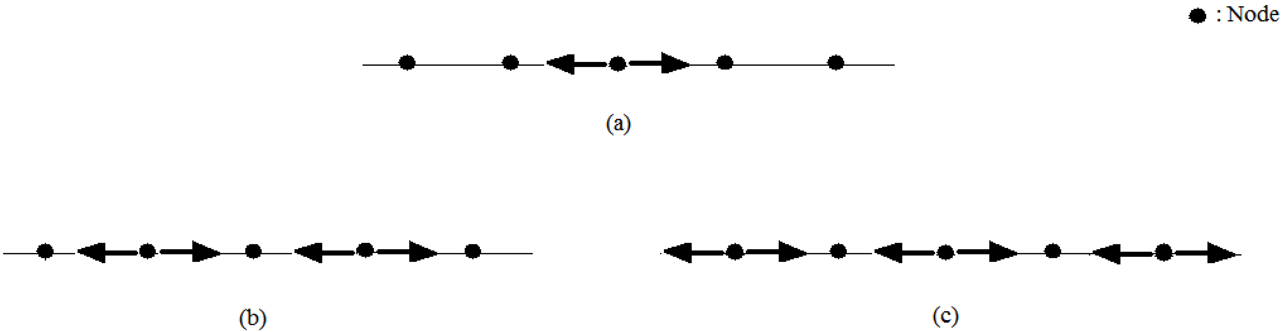
In TLM, each transmission line is excited with a pulse which will be monitored throughout the network. The injected pulse propagates along the line until it reaches a discontinuity (node) where it disperses [27]. Each reflected pulse moves back along the line and becomes incident on the adjacent node after a time step Δt(s), and so on [19,21] (Figure 1). At each iteration k (Equation (11)), the TLM routine calculates the incoming pulses to determine the evolution of the physical quantity at a given point, then the reflected pulses in preparation for the next iteration [26,28] TLM can be one-dimensional, two-dimensional, or three-dimensional [11,28].

$$k=\frac{t}{\Delta t}$$

(11)

TLM has been compared with various other numerical methods such as the Finite Difference method (FDTD) [22,26,29]. These comparisons define the power of this method to the studied case.

Figure 1. Dispersion of an injected pulse. (a) pulse reflection; (b) the first iteration result; and (c) the second iteration result.

Figure 1. Dispersion of an injected pulse. (a) pulse reflection; (b) the first iteration result; and (c) the second iteration result.

2.2.2. TLM Model for Pollutant Dispersion Phenomenon

Early TLM models for dispersion of a physical quantity, proposed the study of both phenomena (advection and diffusion) separately [30,31]. They were based on the concept that transfers the physical content of each node to the node adjacent downstream along the flow direction. According to the results obtained by de Cogan and Henini [11,31], this approach is poor. 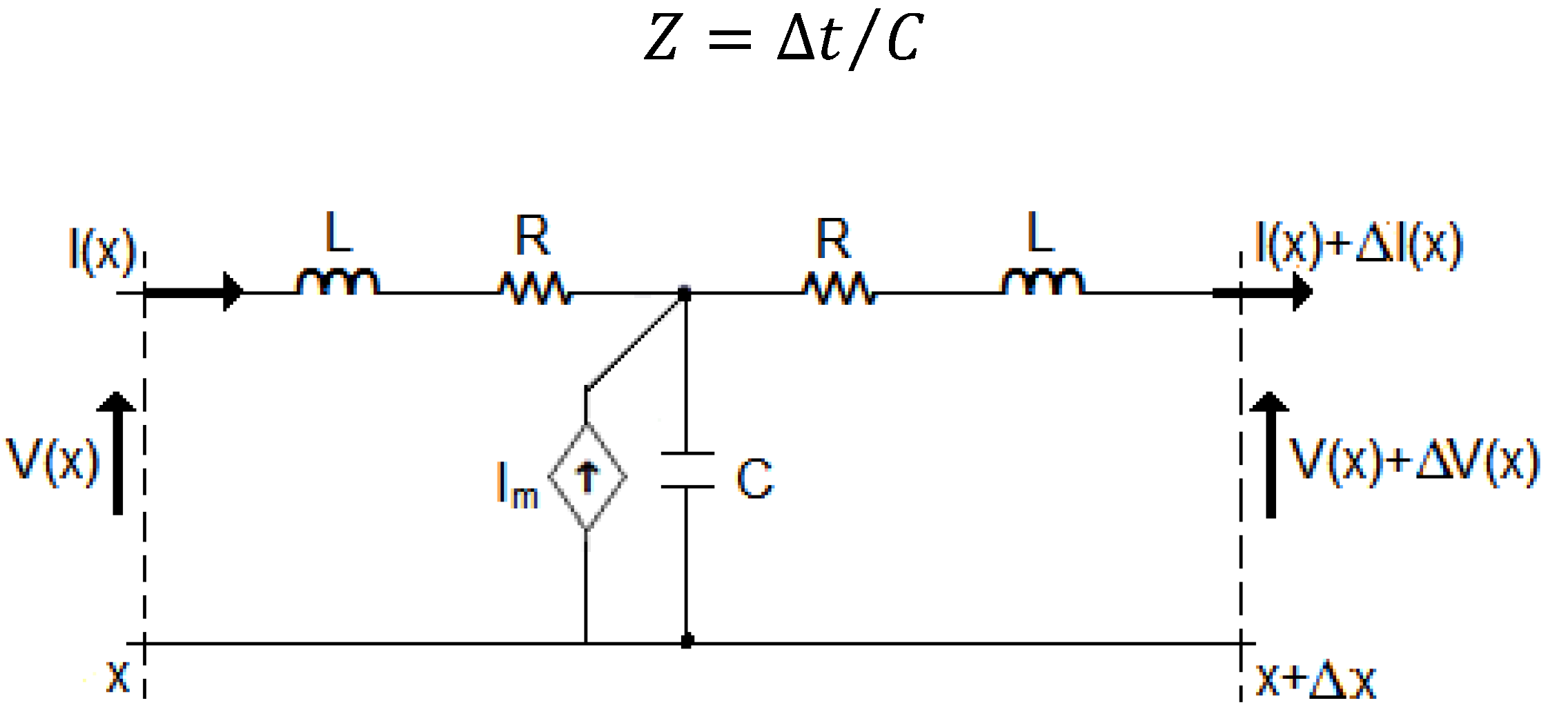An alternative method is proposed [11,32] where the TLM model of dispersion is identical to the TLM model for diffusion with an added current generator I_m(A) at each node. 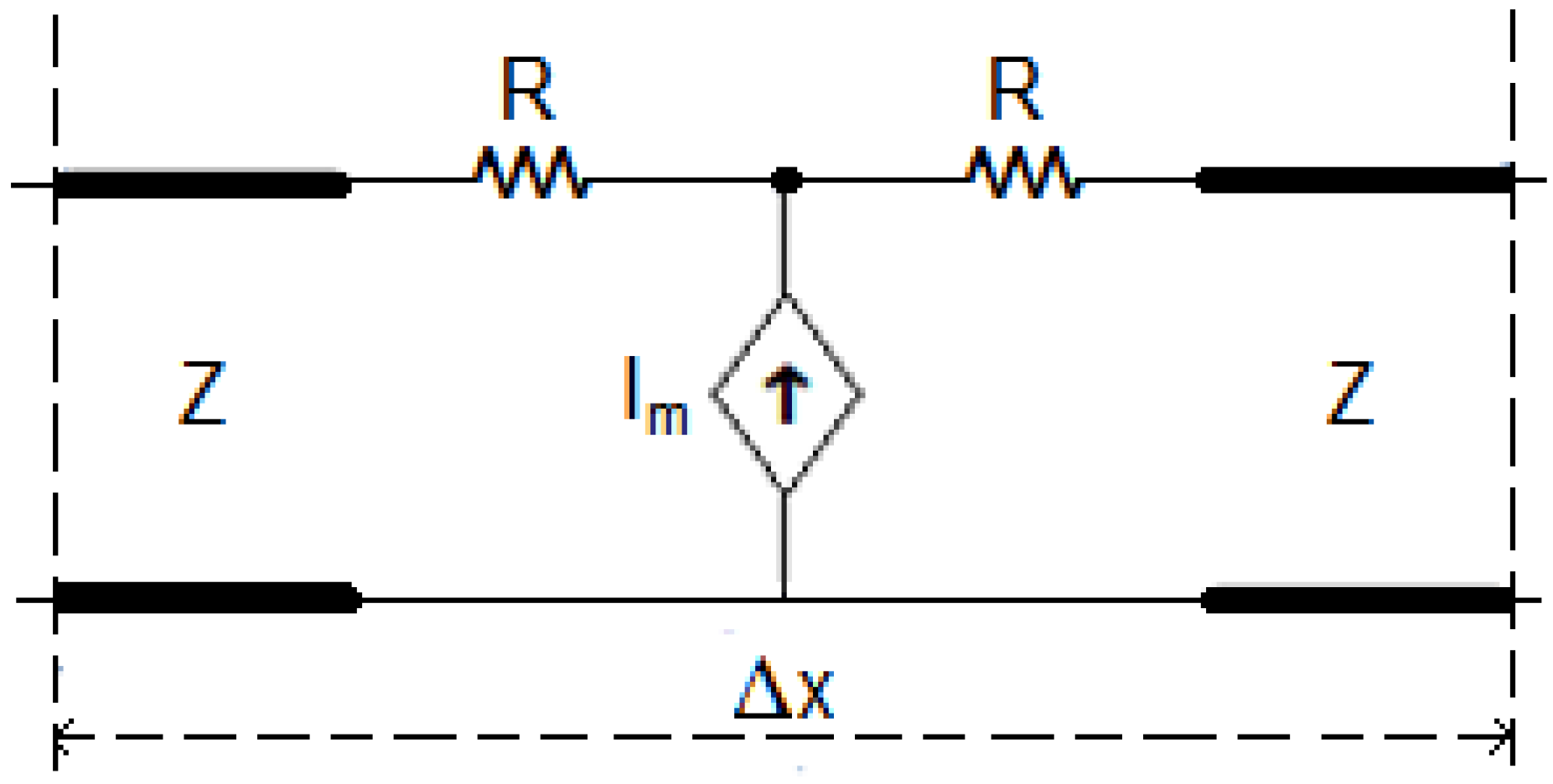Hence, a TLM model of a pollutant dispersion phenomenon is a perfectly insulated transmission line (conductance G(Ω) null) of length Δx(m), that is electrically represented by two resistors R(Ω), two inductors L(H), and a capacitor C(F) (Figure 2). The TLM node is given on Figure 3, where I(x), V(x), and Z are, respectively, the intensity of current (A), the voltage (Volt), and the characteristic impedance (Ω) of the line. The latter is defined by the relation from Equation (12).

$$Z=\Delta t/C$$

(12)

Figure 2. Electrical representation of TLM dispersion model.

Figure 2. Electrical representation of TLM dispersion model.

Figure 3. TLM dispersion node.

Figure 3. TLM dispersion node.

R_d, C_d, and L_d are, respectively, distributed resistance, capacitance, and inductance over the entire length Δx of the transmission line and are given by the following relationships:

$$R_{d }=2R/\Delta x$$

(13)

$$C_{d }=C/\Delta x$$

(14)

$$L_{d }=2L/\Delta x$$

(15)

The variation of the voltage on a piece of transmission line is equal to the sum of the voltage variation due to the inductance and the voltage drop across the resistor as shown in Equation (16):

$$\frac{\partial V\left(x,t\right)}{\partial x}=-R_{d}I\left(x,t\right)-L_d\frac{\partial I\left(x,t\right)}{\partial t}$$

(16)

The current intensity variation flowing through this piece of transmission line is equal to the current flowing through the capacitor to which we add a current generator I_m at the node (n) as indicated by Equation (17):

$$\frac{\partial I\left(x,t\right)}{\partial x}=\frac{I_m\left(x,t\right)}{\Delta x}-C_d\frac{\partial V\left(x,t\right)}{\partial t}$$

(17)

where,

$$I_m\left(x,t\right)=g_m\Delta V\left(x,t\right)$$

(18)

$g_m$: Transconductance (Ω).

If ∆x→0, Equation (17) becomes:

$$\frac{\partial I\left(x,t\right)}{\partial x}=g_m\frac{\partial V\left(x,t\right)}{\partial x}-C_d\frac{\partial V\left(x,t\right)}{\partial t}$$

(19)

If we neglect the influence of the inductance by taking a small enough time step, the combination of Equation (16) and Equation (19) gives:

$$\frac{{\partial }^{2}V\left(x,t\right)}{\partial x^2}+g_m{R}_d\frac{\partial V\left(x,t\right)}{\partial x}=C_d{R}_d\frac{\partial V\left(x,t\right)}{\partial t}$$

(20)

This equation is similar to Equation 3 and, therefore, we can model a phenomenon of pollutant dispersion by an electrical equivalent.

The addition of a current generator produces an additional voltage $\left[I_m\frac{R+Z}{2}\right]$ at node (n). Hence, the total pulse at iteration k, ${}_{k}V\left(\text{n}\right)$ becomes:

$${}_{k}V\left(n\right)=\left({}_{k}V_1^i\left(n\right)+{}_{k}V_2^i\left(n\right)\right)+I_m\left(n\right)\frac{R+Z}{2}$$

(21)

$$I_m\left(n\right)=g_m\left[\frac{{}_{k-1}V\left(n+1\right)-{}_{k-1}V\left(n-1\right)}{2}\right]$$

(22)

${}_{k}V_1^i\left(n\right)$ and ${}_{k}V_2^i\left(n\right)$ are, respectively, the incident pulses on left and right of node (n) at iteration k. ${}_{k-1}V\left(n+1\right)$ and ${}_{k-1}V\left(n-1\right)$ are the pulses at nodes adjacent (n+1) and (n–1) at iteration k–1.

Pulses reflected on left and right of node (n) at iteration k: ${}_{k}V_1^r\left(n\right)$ and ${}_{k}V_2^r\left(n\right)$ are given by Equation (23) and Equation (24):

$${}_{k}V_1^r\left(n\right)=\frac{Z}{R+Z}{}_{k}V\left(n\right)+\frac{R-Z}{R+Z}{}_{k}V_1^i\left(n\right)$$

(23)

$${}_{k}V_2^r\left(n\right)=\frac{Z}{R+Z}{}_{k}V\left(n\right)+\frac{R-Z}{R+Z}{}_{k}V_2^i\left(n\right)$$

(24)

The reflected pulses become incident on adjacent nodes at next iteration. ${}_{k+1}V_1^i\left(n\right)$ and ${}_{k+1}V_2^i\left(n\right)$ are incident pulses on left and right of node (n) at iteration k+1 and are given by Equation (25) and Equation (26):

$${}_{k+1}V_1^i\left(n\right)={}_{k}V_2^r\left(n-1\right)$$

(25)

$${}_{k+1}V_2^i\left(n\right)={}_{k}V_1^r\left(n+1\right)$$

(26)

${}_{k}V_2^r\left(n-1\right)$ and ${}_{k}V_1^r\left(n+1\right)$ are respectively reflected pulses on right of node (n–1) and left of node (n+1).

Equations (21) to (26) form the TLM algorithm used to solve a wide variety of dispersion problems, such as chromatographic processes, heat exchanges, heat flow and diffusion of electric species in semiconductors [32,33]. Analogy between Equation (3) and Equation (20) gives:

$$D_L=1/C_d{R}_d$$

(27)

$$U=-g_{\text{m}}/C_d$$

(28)

$$c\left(x,t\right)=V\left(x,t\right)$$

(29)

$$\partial c\left(x,t\right)/\partial x=-I\left(x,t\right)R_d$$

(30)

According to the Courant-Friedrichs-Lewy stability criterion [11,34], TLM Dispersion models are stable if: $1\ge 2r\ge s^2$, where s is the convection number (Equation (31)) and r is the diffusion number (Equation (32)).

$$s=\frac{U \Delta t}{2\Delta x}$$

(31)

$$r=\frac{D \Delta t}{\Delta x^2}$$

(32)

2.2.3. TLM Initial and Boundary Conditions

In the TLM method, the conditions cited in paragraph (2.1.3) are equivalent to:

$$V_1^i\left(1\right)=V_2^i\left(1\right)=C_0/2$$

(33)

$$V\left(1\right)=C_0$$

(34)

The first node (n = 1) is the tracer dumping point (x = 0) with the boundary condition:

$$V_1^i\left(1\right)=-V_1^r\left(1\right)$$

(35)

At the last node (n), the boundary condition is:

$$V_2^i\left(n\right)=-V_2^r\left(n\right)$$

(36)

The incident pulse returns with the same magnitude but opposite sign. In TLM, this boundary corresponds to a short circuit where the reflection coefficient Γ is equal to −1 [11,20,21].

2.2.4. TLM parameters Optimization

The TLM dispersion model is applied on experimental data of Atkinson and Davis [12] and uses the input data of Table 2. The injected total tension is equivalent to initial concentration at dumping point (Equation (29)). The tracer is poured into an elementary volume of the river ∆v = ∆x∆y∆z, where ∆y and ∆z are, respectively, the width (m) and depth (m) of the river at the dumping point. This dilution leads to an initial concentration of the tracer of 1110 μg/L at dumping point.

Table 2. TLM input data.

Input Data	Parameter/Unit	Value
Experiment duration	t (s)	35,000
Time step	∆t (s)	10
Test distance	ℓ (m)	14,000
Distance step	∆x (m)	25
Characteristic impedance	Z (Ω)	10
Injected total tension	V(1) (Volt)	1110

Table 2. TLM input data.

Input Data	Parameter/Unit	Value
Experiment duration	t (s)	35,000
Time step	∆t (s)	10
Test distance	ℓ (m)	14,000
Distance step	∆x (m)	25
Characteristic impedance	Z (Ω)	10
Injected total tension	V(1) (Volt)	1110

The TLM parameters R_d, g_m, and initial total tension V₀ have been optimized to keep the modeling simple. In TLM technique, the time step ∆t must be less than the time constant (RC) leading to a choice of R_d > 0.8. The conductance is the resistance inverse, so g_m < 1.25. The initial total tension at each node must be inferior to the injected total tension (first node), so V₀ (n ≠ 1) < 1110.

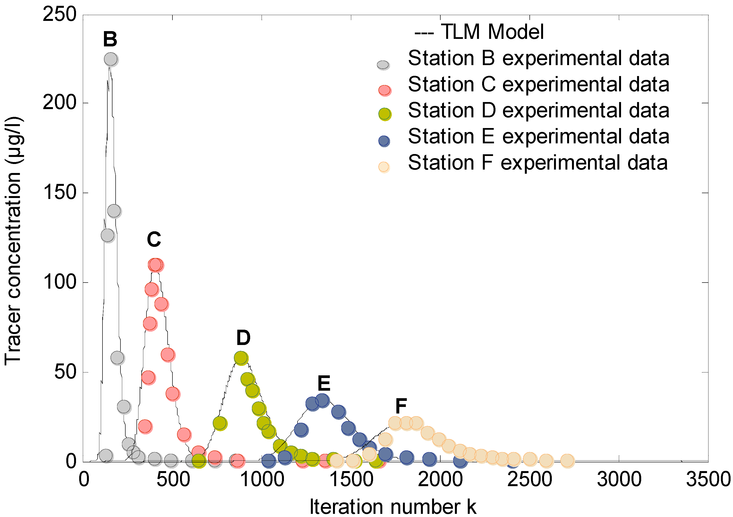
The TLM model, with the input data of Table 2 and the above TLM parameters, is run. The obtained TLM results V = f(k) are compared to the experimental data of Atkinson and Davis C = f(t), i.e., the TLM characteristic parameters (k₀, V_max, k_p, k_f) are compared to the electrical equivalents of experimental characteristic parameters (t₀, C_max, t_p, t_f) (Table 1). The electrical equivalents (k'₀, V'_max, k'_p, k'_f) are deduced from Equation (11) and Equation (29). The optimized TLM parameters (R_d, g_m, and V₀) correspond to the minimal values (∆k₀, ∆V_max, ∆k_p, ∆k_f).

This optimization is acceptable if we can validate, statistically, and interpret, physically, the differences between the experimental parameters and the physical equivalents of TLM parameters which are calculated using Equation (27), Equation (28), and Equation (29).

2.3. Statistical Tests for TLM Model Validation

The model performance is analyzed by comparing, for each station, observed data (experimental data of Atkinson and Davis (Table 3)) with TLM model predictions (physical equivalents of optimal TLM results (Table 4)) for the following parameters: flow velocity (U_tlm and U), longitudinal dispersion coefficient (D_tlm and D_L), maximum concentration (C_maxtlm and C_max), peak time (t_ptlm and t_p), start time of pollution (t_0tlm and t₀), and end time of pollution (t_ftlm and t_f).

The statistical indices are the basic tools for analyzing the model quality [6,14,35,36,37]. The following tests have been chosen: The coefficient of divergence R_div with R_div >1 (R_div < 1) indicates an over-prediction (under-prediction) of a value; the mean percentage error E(%) representing a convenient model when it is small; the Mean Relative Square Error MRSE indicating a successful model if it is close to 0; the Factor Of EXcedence FOEX(%), signifying an overestimation (underestimation and/or correct estimation) of all values when it is equal to 100% (0%); the factor of two FA₂(%) representing a reliable model if it is close to 100% and finally the scatter diagram indicating a situation of overestimation (underestimation) when the point is above (below) “y = x” line.

3. Results and Discussion

3.1. Determination of Experimental Parameters

The experimental concentration data of Atkinson and Davis [12] have been considered to calculate at each station: $\overline{t}$ by Equation (9), ${\text{σ}}_t^2$ by Equation (8), and U by Equation (7). D_L is determined using Equation (4). The results are presented in Table 3:

Table 3. Experimental values of flow velocities and longitudinal dispersion coefficients.

Station	U (m/s)	DL (m2/s)
B	0.71	18.76
C	0.68	23.39
D	0.45	11.47
E	0.55	62.62
F	0.50	22.97
G	0.72	−101.48

Table 3. Experimental values of flow velocities and longitudinal dispersion coefficients.

Station	U (m/s)	DL (m2/s)
B	0.71	18.76
C	0.68	23.39
D	0.45	11.47
E	0.55	62.62
F	0.50	22.97
G	0.72	−101.48

The flow velocity varies from one station to another, and so does the longitudinal dispersion coefficient with distance x. These two parameters depend on the roughness and the variable geometry of the river. The value of longitudinal dispersion coefficient of station E is very high because of an obvious change in geometry of the river. The value of longitudinal dispersion coefficient of station G is negative. According to Atkinson and Davis [12], the time was insufficient to carry out all the necessary measurements at station G; thus, the dispersion monitoring was incomplete. The following day, measurements were remade only at two stations: station F, to compare the results of the two experiments and describe the dispersive behavior of the test channel, and station G, to complete the concentration recording according to time. The comparison of results showed that the dispersive behavior of the test channel is reproducible. Finally, all the results were compiled by taking measurements of the first experiment at the stations A to F and adjusted measurements of the second experiment at the station G. Since the longitudinal dispersion coefficient value depends essentially on the spatio-temporal monitoring of concentrations, the lack of reliable experimental data at station G led to obtain a negative coefficient of longitudinal dispersion. Thus, station G will be ignored from our comparative study.

3.2. Determination of TLM Parameters

Figure 4 shows the optimized TLM results and Table 4 their physical equivalents.

Figure 4. TLM modeling and experimental data of Atkinson and Davis. The total tension (tracer concentration) is traced according to the iteration number k at stations B, C, D, E, and F.

Figure 4. TLM modeling and experimental data of Atkinson and Davis. The total tension (tracer concentration) is traced according to the iteration number k at stations B, C, D, E, and F.

Globally, there is a good agreement between the TLM results and experimental data. For stations E and F, the TLM curve is slightly shifted from the experimental curve; this means that the TLM model underestimates the beginning and end of pollution and gives a polluting trail shorter than that observed with an overestimation of flow velocity. This is certainly due to the sudden and obvious change of the channel geometry at 6.5 km from the injection point (upstream of the station E); downstream from this distance, the channel section is bigger, and downstream from the station E, the channel is wider and more sinusoidal, but the TLM model does not take into account the channel geometry which strongly influences the dispersion evolution [10,17,38,39]. Furthermore, between 6.5 km from the injection point and the station E, the channel is much deeper because its bed is composed of a series of riffles and pools storage areas or dead zones [9], which retain pollutant then release it after some time, with such effect stretching, longitudinally, the pollution slick leading to the slight difference between the experimental and modeling curves; but the TLM model does not take into consideration the channel topography which strongly influences the dispersive behavior of the channel [7,9,16,40].

Table 4. Optimized TLM parameters and their physical equivalents.

Station	TLM Parameters			Physical Equivalents
	−gm (Ω)	Rd (Ω)	V0(Volt)	Utlm (m/s)	Dtlm(m2/s)	C0tlm (μg/L)
B	0.03	1.33	990	0.76	18.76	990
C	0.03	0.89	863.5	0.70	28.2	863.5
D	0.02	1.04	690	0.59	24	690
E	0.02	0.83	522	0.576	30	522
F	0.02	0.89	370	0.56	28	370

Table 4. Optimized TLM parameters and their physical equivalents.

Station	TLM Parameters			Physical Equivalents
	−gm (Ω)	Rd (Ω)	V0(Volt)	Utlm (m/s)	Dtlm(m2/s)	C0tlm (μg/L)
B	0.03	1.33	990	0.76	18.76	990
C	0.03	0.89	863.5	0.70	28.2	863.5
D	0.02	1.04	690	0.59	24	690
E	0.02	0.83	522	0.576	30	522
F	0.02	0.89	370	0.56	28	370

It’s important to remark that U_tlm, D_tlm, and C_0tlm are, respectively, the flow velocity, the longitudinal dispersion coefficient, and the initial concentration predicted by the TLM model.

Our model does not take into account the variable geometry and topography of the channel in order to reduce the model input data, since a model is just required to be able to provide useful predictions in case of emergencies. Actually, the study of complex geomorphologic flows requires specific computational methods [10,41] that take into account: Geometry, curvature, meandering, flooding conditions, bed topography, riparian vegetation, and secondary flows that influence the meandering evolution [42].

3.3. TLM Model Performance

The statistical tests results are given in Table 5 and shown in Figure 5.

Table 5. Statistical tests for flow velocity, longitudinal dispersion coefficient and maximum concentration.

Parameters	Indices	B	C	D	E	F	Average
Flow velocity (Utlm, U)	Rdiv	1.07	1.03	1.31	1.05	1.12	1.12
	E (%)	7.00	2.90	31.10	4.70	12.0	11.60
	MRSE	0.02
	FOEX (%)	100
	Fa2 (%)	100
Longitudinal dispersion coefficient (Dtlm, DL)	Rdiv	1.00	1.21	2.09	0.48	1.22	1.20
	E (%)	0.00	20.60	109.20	52.10	21.90	40.80
	MRSE	0.21
	FOEX (%)	60
	Fa2 (%)	60
Maximum concentration (Cmaxtlm, Cmax)	Rdiv	1.00	1.00	1.00	1.00	1.00	1.00
	E (%)	0.00	0.00	0.10	0.00	0.00	0.00
	MRSE	0.00
	FOEX (%)	0
	Fa2 (%)	100

Table 5. Statistical tests for flow velocity, longitudinal dispersion coefficient and maximum concentration.

Parameters	Indices	B	C	D	E	F	Average
Flow velocity (Utlm, U)	Rdiv	1.07	1.03	1.31	1.05	1.12	1.12
	E (%)	7.00	2.90	31.10	4.70	12.0	11.60
	MRSE	0.02
	FOEX (%)	100
	Fa2 (%)	100
Longitudinal dispersion coefficient (Dtlm, DL)	Rdiv	1.00	1.21	2.09	0.48	1.22	1.20
	E (%)	0.00	20.60	109.20	52.10	21.90	40.80
	MRSE	0.21
	FOEX (%)	60
	Fa2 (%)	60
Maximum concentration (Cmaxtlm, Cmax)	Rdiv	1.00	1.00	1.00	1.00	1.00	1.00
	E (%)	0.00	0.00	0.10	0.00	0.00	0.00
	MRSE	0.00
	FOEX (%)	0
	Fa2 (%)	100

Figure 5a presents the comparison between the predicted and experimental values of flow velocity. According to Figure 5a and Table 5, the scatter diagram and FOEX indicate that all the experimental values are over-predicted with a mean percentage error equal to 11.6%. The model seems to be able to simulate the observed values of flow velocity well at stations C and E, with a weak over-estimation at stations B and F, and with a significant over-prediction at station D. This may indicate that at station D, the predicted tracer cloud disperses more quickly than the observed one. The experimental flow velocity at station D is the smallest (Table 3) so the passage of the tracer could is slow. It can be slowed down by the different river morphologies: sinuosity, topography, dead zones, expansions and contractions; these aspects are known to affect the distribution profiles of velocity. Thus, the difference between TLM and experimental values can be attributed to the fact that the 1D-TLM model does not take into account these aspects. The values of Fa₂, MRSE, and E indicate that the model representation of the experimental flow velocity is acceptable.

Figure 5. Scatter diagrams for (a): flow velocity; (b): longitudinal dispersion coefficient; (c): maximum concentration; (d): peak time; (e): pollution start time; and (f): pollution end time.

Figure 5. Scatter diagrams for (a): flow velocity; (b): longitudinal dispersion coefficient; (c): maximum concentration; (d): peak time; (e): pollution start time; and (f): pollution end time.

On Figure 5b, the predicted longitudinal dispersion coefficients are plotted against the observed ones. According to Figure 5b and Table 5, the scatter diagram and FOEX indicate that there are situations of over and under-estimation with a mean percentage error of 40.78%. The model gives a good estimate of the longitudinal dispersion coefficient for station B, but slightly over-predicts the coefficients of stations C and F, over-predicts the coefficient for station D, and under-predicts that of station E. The differences between the predicted and observed values are remarkable for the two stations D and E. The comparison of these two stations to the others shows that station D has the smallest coefficient, while station E is characterized by the highest coefficient (Table 3). Looking at station D, its smallest flow velocity has led to a smaller coefficient since D_L decreases with U. The overestimation of the flow velocity explains the overestimation of the longitudinal dispersion coefficient at this station. For station E, its coefficient is the highest because of an obvious and sudden change in river geometry upstream of the station E at 6.5 km from the injection point. In this region, the channel is much deeper and starts to widen; station E has the biggest section. The longitudinal dispersion coefficient depends on the width and depth of the channel; thus, it is strongly related to the channel geometry. Therefore, the difference between the predicted and observed longitudinal dispersion coefficients at station E is due to our model not taking into account the channel geometry. The values of Fa₂, MRSE, and E indicate that the model representation of the experimental longitudinal dispersion coefficients is fairly acceptable. Moreover, the numerical estimation of this coefficient is very difficult; in the literature [7,8,9,14,17,38,43,44,45,46] for natural rivers, there is a great disparity between the values of longitudinal dispersion coefficients calculated by different methods and empirical formulas. This shows that such a coefficient is difficult to estimate, its experimental determination is the fairest approach because it is based on spatio-temporal monitoring of pollutant concentrations in streams with the real effect of skewness, topography, and water storage areas.

Figure 5c shows the predicted maximum concentrations compared to the experimental ones and Figure 5d presents the comparison between predicted and experimental values of the maximum concentration time (peak time). The scatter diagram of Figure 5c and the statistical indices of Table 5 show that the TLM model correctly predicted all maximum concentrations with a null mean percentage error. The scatter diagram on Figure 5d shows that the maximum concentration time predicted by TLM model is in good agreement with that obtained experimentally. E is equal to 0.8%, MRSE is zero, FOEX is null, indicating that there is no overestimation, and Fa₂ factor is equal to 100%. All the statistical tests indicate that the model provides a very well representation for the experimental maximum concentrations and their peak times. The principal role of a pollutant model is to correctly give the pollution degree (maximum concentration and its peak time) at a given distance; the hereby-presented original model satisfies this requirement.

Figure 5e,f present the comparison between predicted and experimental time values of the pollution start and pollution end, respectively. The scatter diagrams show that the model slightly underestimates the pollution start time and considerably underestimates the pollution end time. This may indicate that the predicted cloud passage across each sampling station is earlier than the observed cloud passage and the model predicts a trail of pollutant shorter than that observed experimentally. This can be explained by the fact that the long profile of the riverbed consists of a series of storage areas (dead zones and pools) which retained the tracer and released it after a certain duration; this retarded the cloud passage at each station and longitudinally stretched the pollutant slick. Thus, the difference between the TLM and the experimental values is due to the fact that the TLM model does not take into account the phenomena of roughness and dead zones. For the pollution start time, E is equal to 13.8%, MRSE is 0.04, FOEX is null, confirming that all the experimental values are under-predicted, and Fa₂ factor is equal to 100%. For the pollution end time, E is equal to 36%, MRSE is 0.32, FOEX is null, and Fa₂ factor is equal to 60%. These statistical tests show that the model provides a good estimate of pollution start time but less of an estimate of the pollution end time. It is preferable for a pollution model to predict early tracer cloud passage so one can react as quickly as possible to preserve the environment. The hereby-presented original model fulfills this demand.

3.4. TLM Model Stability

In the considered case study, the condition of the Courant-Friedrichs-Lewy stability criterion [29] is respected for every station (Table 6).

Table 6. Convection and diffusion numbers.

Stations	s	r
B	0.15	0.30
C	0.14	0.45
D	0.12	0.38
E	0.12	0.48
F	0.11	0.45

Table 6. Convection and diffusion numbers.

Stations	s	r
B	0.15	0.30
C	0.14	0.45
D	0.12	0.38
E	0.12	0.48
F	0.11	0.45

3.5. Final TLM Model

Differences between TLM parameters and experimental parameters are statistically validated and physically interpreted as due to neglecting some minor phenomena characterizing pollutant dispersion in a river. Therefore, we defined α, β, and γ as factors representing ones of these neglected phenomena with α = D_L/D_tlm, β = U/U_tlm, and γ = C₀/C_0tlm. These factors (Table 7) are different because of the channel geometry and topology variation from a station to another.

Table 7. Factors α, β and γ.

Station	α	β	γ
B	1	0.93	1.12
C	0.83	0.97	1.29
D	0.48	0.76	1.61
E	2.09	0.95	2.13
F	0.82	0.89	3.00

Table 7. Factors α, β and γ.

Station	α	β	γ
B	1	0.93	1.12
C	0.83	0.97	1.29
D	0.48	0.76	1.61
E	2.09	0.95	2.13
F	0.82	0.89	3.00

Considering these factors, the TLM model equations become:

$${}_{k}V\left(n\right)=\left({}_{k}V_1^i\left(n\right)+{}_{k}V_2^i\left(n\right)\right)+I_m\left(n\right)\frac{\propto R+Z}{2}$$

(37)

$$I_m\left(n\right)={\text{β}}^{-1} {\text{g}}_m\left[\frac{{}_{k-1}V\left(n+1\right)-{}_{k-1}V\left(n-1\right)}{2}\right]$$

(38)

$${}_{k}V_1^r\left(n\right)=\frac{Z}{\propto R+Z}{}_{k}V\left(n\right)+\frac{\propto R-Z}{\propto R+Z}{}_{k}V_1^i\left(n\right)$$

(39)

$${}_{k}V_2^r\left(n\right)=\frac{Z}{\propto R+Z}{}_{k}V\left(n\right)+\frac{\propto R-Z}{\propto R+Z}{}_{k}V_2^i\left(n\right)$$

(40)

The initial conditions become:

$$V_1^i\left(1\right)=V_2^i\left(1\right)=C_0/2\gamma \to V\left(1\right)=C_0/\gamma$$

(41)

The boundary conditions are:

$$V_1^i\left(1\right)=-V_1^r\left(1\right)$$

(42)

$$V_2^i\left(n\right)=-V_2^r\left(n\right)$$

(43)

This new model can present the pollution evolution at each station by knowing only the channel length, poured pollutant quantity, longitudinal dispersion coefficient, and flow velocity.

4. Conclusions

The proposed one-dimensional TLM model provides a good estimate of pollutant longitudinal dispersion in the far field zone of a river, such as the river Severn (UK). Usually, this model overestimates flow velocities and longitudinal dispersion coefficients but describes quite well the evolution of maximum concentrations over time. It underestimates time of start and end of pollution. This overestimation or underestimation may be related to the natural aspects of the river such as roughness, topography, geometry, and dead zones that longitudinally stretch the pollutant slick. Statistical tests indicate that the model is quite efficient and reliable. Generally, a model representing a phenomenon of pollution should preferably underestimate pollution start time and peak time, and not the other way, so to stress the situation and, hence, respond as quickly as possible. According to the Courant-Friedrichs-Lewy stability criterion, our TLM Dispersion model is stable. Therefore, the hereby-presented original model with few input data can be used to predict the spatiotemporal evolution of a pollutant slick in natural streams with a dynamic similar to that of the river Severn (that is, the first considered case study).

References

1. Chapra, S.C. Surface Water-Quality Modeling; McGraw-Hill Series in Water Resources and Environmental Engineering: New York, NY, USA, 1997. [Google Scholar]
2. Fischer, H.B.; List, E.J.; Koh, R.C.Y.; Imberger, J.; Brooks, N.H. Mixing in Inland and Coastal Waters; Academics Press: San Diego, CA, USA, 1979. [Google Scholar]
3. Graf, W.H. Fluvial Hydraulics: Flow and Transport Processes in Channels of Simple Geometry; Wiley: Hoboken, NJ, USA, 1998. [Google Scholar]
4. Runkel, R.L.; Broshears, R.E. One-Dimensional Transport with Inflow and Storage (OTIS)—A Solute Transport Model for Small Streams; University of Colorado: Boulder City, CO, USA, 1991. [Google Scholar]
5. Marsalek, J.; Sztruhar, D.; Giulianelli, M.; Urbonas, B. Enhancing Urban Environment by Environmental Upgrading and Restoration; Kluwer Academic Publishers: Dordrecht, The Netherlands, 2004. [Google Scholar]
6. Jabbour, D. Etude Expérimentale et Modélisation de la Dispersion en Champ Lointain Suite à un Rejet Accidentel d’un Polluant Miscible Dans un Cours d’eau: Application à la Gestion de Crise. Ph.D. Thesis, University of Provence, Aix-en-Provence, France, January 2006. [Google Scholar]
7. Shen, C.; Niu, J.; Anderson, E.J.; Phanikumar, M.S. Estimating longitudinal dispersion in rivers using acoustic doppler current profilers. Adv. Water Resour. 2010, 33, 615–623. [Google Scholar] [CrossRef]
8. Etemad-Shahidi, A.; Taghipour, M. Predicting longitudinal dispersion coefficient in natural streams using M5’ Model Tree. J. Hydraul. Eng. 2012, 138, 542–554. [Google Scholar] [CrossRef]
9. Rodrigues, P.P.G.W.; González, Y.M.; de Sousa, E.P.; Neto, F.D.M. Evaluation of dispersion parameters for river Sao Pedro, Brazil, by the simulated annealing method. Inverse Probl. Sci. Eng. 2013, 21, 34–51. [Google Scholar] [CrossRef]
10. Tealdi, S.; Camporeale, C.; Perucca, E.; Ridolfi, L. Longitudinal dispersion in vegetated rivers with stochastic flows. Adv. Water Resour. 2010, 33, 562–571. [Google Scholar] [CrossRef]
11. De Cogan, D. Transmission Line Matrix (TLM) Techniques for Diffusion Applications; The Gordon and Breach Science Publishers: Amsterdam, The Netherlands, 1998. [Google Scholar]
12. Atkinson, T.C.; Davis, P.M. Longitudinal dispersion in natural channels: 1. Experimental results from the river Severn, UK. Hydrol. Earth Syst. Sci. 2000, 4, 345–353. [Google Scholar] [CrossRef]
13. Fischer, B.H. Longitudinal Dispersion in Laboratory and Natural Streams; California Institute of Technology: Pasadena, CA, USA, 1966. [Google Scholar]
14. Perucca, E.; Camporeale, C.; Ridolfi, L. Estimation of the dispersion coefficient in rivers with riparian vegetation. Adv. Water Resour. 2009, 32, 78–87. [Google Scholar] [CrossRef]
15. Pathak, S.K.; Pande, P.K.; Kumar, S. Effect of circulation on longitudinal dispersion in open channel. In Proceedings of the 6th Australasian Hydraulics and Fluid Mechanics Conference, Adelaide, Australia, 5–9 December 1977; pp. 597–600.
16. Davis, P.M.; Atkinson, T.C.; Wigley, T.M.L. Longitudinal dispersion in natural channels: 2.The roles of shear flow dispersion and dead zones in the river Severn, UK. Hydrol. Earth Syst. Sci. 2000, 4, 355–371. [Google Scholar] [CrossRef]
17. Baek, K.O.; Seo, I.W. Routing procedures for observed dispersion coefficients in two-dimensional river mixing. Adva. Water Resour. 2010, 33, 1551–1559. [Google Scholar] [CrossRef]
18. International Organization for Standardization (ISO). Mesure de Débit Des Liquides Dans Les Canaux Découverts. Longueur de Bon Mélange d’un Traceur; TR 11656-1993; International Organization for Standardization: Geneva, Switzerland, 1993. (In French) [Google Scholar]
19. Toledo-Redondo, S.; Salinas, A.; Morente-Molinera, J.A.; Méndez, A.; Fornieles, J.; Portí, J.; Morente, J.A. Parallel 3D-TLM algorithm for simulation of the earth-ionosphere cavity. J. Comput. Phys. 2013, 236, 367–379. [Google Scholar] [CrossRef]
20. Amri, A.; Saidane, A.; Pulko, S. Thermal analysis of a three-dimensional breast model with embedded tumour using the transmission line matrix (TLM) method. Comput. Biol. Med. 2011, 41, 76–86. [Google Scholar] [CrossRef] [PubMed]
21. Feradji, A.; Pulko, S.H.; Saidane, A.; Wilkinson, A.J. Transmission line matrix modelling of self heating in multi-finger 4H-SiC MESFETs. J. Appl. Sci. 2012, 12, 32–39. [Google Scholar] [CrossRef]
22. Rao, R.S.; Subbaiah, P.V.; Rao, B.P. Electromagnetic transient scattering analysis in time-domain comparison of TLM and TDIE methods. J. Comput. Electron. 2012, 11, 315–320. [Google Scholar]
23. Johns, P.B.; Beurle, R.L. Numerical solution of 2-dimensional scattering problems using a transmission line matrix. Proc. IEEE 1971, 118, 1203–1208. [Google Scholar] [CrossRef]
24. Guillaume, G. Application de la Méthode TLM à la Modélisation de la Propagation Acoustique en Milieu Urbain. Ph.D. Thesis, University of Maine, Orono, ME, USA, October 2009. [Google Scholar]
25. Le Maguer, S. Développement de Nouvelles Procédures Numériques Pour la Modélisation TLM: Application à la Caractérisation de Circuits Plaqués et de Structures à Symétrie de Révolution en Bande Millimétrique. Ph.D. Thesis, University of Western Brittany, Brest, France, November 1998. [Google Scholar]
26. Amri, A. Numerical Analysis of Microwave Sintering of Ceramic Materials Using a 3D-TLM Method. Ph.D. Thesis, University USTO-MB, Oran, Algeria, June 2005. [Google Scholar]
27. Aliouat, B.S.; Saidane, A.; Benzohra, M.; Saiter, J.M.; Hamou, A. Dimensional soft tissue thermal injury analysis using transmission line matrix TLM method. Int. J. Numeri. Model. Electron. Netw. Devices Fields 2008, 21, 531–549. [Google Scholar]
28. Christopoulos, C. The Transmission Line Modeling Method TLM; University of Nottingham: Nottingham, UK, 1995. [Google Scholar]
29. Johns, P.B. On the relationship between TLM and finite-difference methods for Maxwell’s equations. IEEE Trans. Microw. Theory Tech. 1987, 35, 60–61. [Google Scholar] [CrossRef]
30. Smith, A. Transmission Line Matrix Modeling, Optimization and Application to Adsorption Phenomena. Bachelor’s Thesis, Nottingham University, Nottingham, UK, July 1988. [Google Scholar]
31. De Cogan, D.; Henini, M. Transmission line matrix TLM: A novel technique for modeling reaction kinetics. Faraday Trans. 2: Mol. Chem. Phys. 1987, 83, 843–855. [Google Scholar] [CrossRef]
32. Al-Zeben, M.Y.; Saleh, A.H.M.; Al-Omar, M.A. TLM modeling of diffusion, drift and recombination of charge carriers in semiconductors. Int. J. Numer. Model. Electron. Netw. Devices Fields 1992, 5, 219–225. [Google Scholar] [CrossRef]
33. Gui, X.; Gao, G.B.; Morkoç, H. Transmission-line matrix method for solving the multidimensional continuity equation. Int. J. Numer. Model. Electron. Netw. Devices Fields 1993, 6, 233–236. [Google Scholar] [CrossRef]
34. Courant, R.; Friedrichs, K.; Lewy, H. On the partial difference equations of mathematical physics. IBM J. Rese. Dev. 1967, 11, 215–234. [Google Scholar] [CrossRef]
35. Mosca, S.; Graziani, G.; Klug, W.; Bellasio, R.; Bianconi, R. A statistical methodology for the evaluation of long range dispersion models: An application to the ETEX exercise. Atmos. Environ. 1998, 32, 4307–4324. [Google Scholar] [CrossRef]
36. Boybeyi, Z.; Ahmad, N.N.; Bacon, D.P.; Dunn, T.J.; Hall, M.S.; Lee, P.C.S.; Sarma, R.A.; Wait, T.R. Evaluation of the operational multiscale environment model with grid adaptivity against the European tracer experiment. J. Appl. Meteorol. 2001, 40, 1541–1558. [Google Scholar] [CrossRef]
37. Duijm, N.J.; Ott, S.; Nielsen, M. An evaluation validation procedures and test parameters for dense gas dispersion models. J. Loss Prev. Process Ind. 1996, 9, 323–338. [Google Scholar] [CrossRef]
38. Bashitialshaaer, R.; Bengtsson, L.; Larson, M.; Persson, K.M.; Aljaradin, M.; Al-Itawi, H.I. Sinuosity effects on longitudinal dispersion coefficient. Int. J. Sustain. Water Environ. Syst. 2011, 2, 77–84. [Google Scholar]
39. Boxall, J.B.; Guymer, I. Longitudinal mixing in meandering channels: New experimental data set and verification of a predictive technique. Water Res. 2007, 41, 341–354. [Google Scholar] [CrossRef] [PubMed]
40. Zhang, W.; Boufadel, M.C. Pool effects on longitudinal dispersion in streams and rivers. J. Water Resour. Prot. 2010, 2, 960–971. [Google Scholar] [CrossRef]
41. Keylock, C.J.; Constantinescu, G.; Hardy, R.J. The application of computational fluid dynamics to natural river channels: Eddy resolving versus mean flow approaches. Geomorphology 2012, 179, 1–20. [Google Scholar] [CrossRef]
42. Chen, D.; Tang, C. Evaluating secondary flows in the evolution of sine-generated meanders. Geomorphology 2012, 163, 37–44. [Google Scholar] [CrossRef]
43. Kashefipour, S.; Falconer, R. Longitudinal dispersion coefficients in natural channels. Water Res. 2002, 36, 1596–1608. [Google Scholar] [CrossRef]
44. Dongsu, K. Assessment of longitudinal dispersion coefficients using acoustic doppler current profilers in large river. J. Hydro-Environ. Res. 2012, 6, 29–39. [Google Scholar]
45. Piotrowski, A.P.; Rowinski, P.M.; Napiorkowski, J.J. Comparison of evolutionary computation techniques for noise injected neural network training to estimate longitudinal dispersion coefficients in rivers. Expert Syst. Appl. 2012, 39, 1354–1361. [Google Scholar] [CrossRef]
46. Azamathulla, H.M.; Ghani, A.A. Genetic programming for predicting longitudinal dispersion coefficients in streams. Water Resour. Manag. 2011, 25, 1537–1544. [Google Scholar] [CrossRef]