Flow Patterns in an Open Channel Confluence with Increasingly Dominant Tributary Inflow

Abstract

Despite the ratio of incoming discharges being recognized as a key parameter in open-channel confluence hydrodynamics, little is known about the flow patterns when the tributary provides more than 90% of the total discharge. This paper offers a systematic study of flow features when the tributary becomes increasingly dominant in a 90° confluence with a fixed concordant bed. Large-eddy simulations are used to investigate the three-dimensional complex flow patterns for three different discharge ratios. It is found that the tributary flow impinges on the opposing bank when the tributary flow becomes sufficiently dominant, causing a recirculating eddy in the upstream channel of the confluence, which induces significant changes in the incoming velocity distribution. Moreover, it results in stronger helicoidal cells in the downstream channel, along with zones of upwelling flow. In turn, the changed flow patterns also influence the mixing layer and the flow recovery. Finally, intermittent events of stronger upwelling flow are discerned. Improved understanding of flow patterns at confluences where the tributary is dominant is applicable to both engineering and earth sciences.

1. Introduction

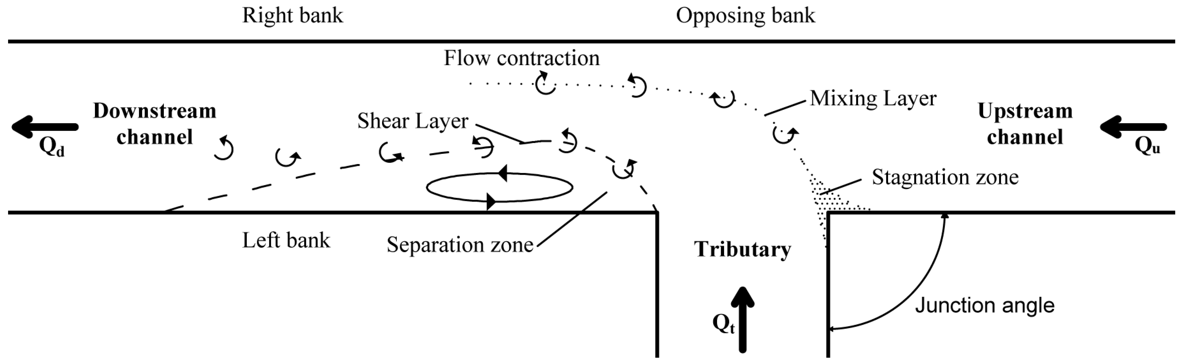
Confluences of open channels are important elements in hydraulic networks of rivers and man-made canals. The associated flow patterns govern the transport of solutes and sediments in the network and influence the water levels of the incoming channels. The flow features that appear in an open channel confluence can be conceptualized as follows (Figure 1 after Best [1]): At the point where the two incoming flows meet, a stagnation zone develops, i.e., a zone of reduced flow velocity. From the stagnation zone, a mixing layer departs, which delineates the merging streams. At the downstream junction corner, the tributary flow may detach, causing the formation of a separation zone. Next to the separation zone, the merging flows passing through a narrowed cross-section are contracted, leading to increased velocities.

Figure 1. Conceptual model of an open channel confluence (after Best [1]).

Figure 1. Conceptual model of an open channel confluence (after Best [1]).

From the very beginning of laboratory research on confluences, starting with Taylor [2], the ratio of incoming discharges has been recognized as a key parameter [1,2,3]. However, laboratory research was mainly performed with discharge ratios in the range of $0.1 \lesssim q \lesssim 0.9$, at least for the case of asymmetrical confluences with a fixed concordant bed and subcritical flow throughout [12]; the type of confluence that will be further considered in this paper. In the above-mentioned equation, the discharge ratio q is defined as the ratio of upstream to downstream channel discharge (see Figure 1):

$$q = \frac{Q_u}{Q_d} = \frac{Q_u}{Q_u+Q_t}$$

(1)

Although it is known that the three-dimensionality of the flow increases with a decreasing discharge ratio, i.e., when the tributary becomes dominant, indications of the flow features at q < 0.1 are scarce. For example, Webber & Greated [3] observed a decreasing accuracy of their theoretical model at lower q. Gurram et al. [6] were the first to provide a qualitative view on the case where q = 0 (i.e., all flow coming from the tributary) by means of photographs. They noted the significant impact of the tributary flow on the opposing wall, and alluded to flow in a mitre bend. The uniqueness of q = 0 has also been demonstrated for transcritical flow [4], where a local maximum in the water height at the opposing wall is found when q = 0, a phenomenon that is absent at the other investigated discharge ratios. Moreover, the flow field indicates inflow from the confluence area into the upstream channel when q = 0. For subcritical flows, Shumate [8] reported that the case q = 0.083 (i.e., the case with the smallest discharge ratio amongst his experiments) did not follow the trends deduced from the cases with higher discharge ratios. He reported the separation zone was shorter than expected due to the reflection of the lateral flow in the upstream channel. All the foregoing elements offer evidence that distinct flow features are present at sufficiently small discharge ratios. However, no systematic study of these patterns has been undertaken.

As preliminary research, Schindfessel et al. [12] experimentally compared two discharge ratios, q = 0.25 and q = 0.05, in a 90° angle confluence flume and found some particularities at the small discharge ratio. The impinging tributary flow led to a recirculating eddy in the upstream channel, as well as to changes in the helicoidal cells.

Field-based research also acknowledged the importance of the discharge ratio (e.g., [14,15]), not only on time-averaged flow, but also on intermittent features [16,17]. According to the literature overview provided by Leite Ribeiro et al. [18], the only morphological study including q < 0.1 was provided by Rhoads et al. [15]. These authors found that low discharge ratios are associated with a distinct bed topography, whereby the scour hole is located close to the opposing bank (seen from the tributary), leading to erosion of that bank in the long term. This is caused by the tributary flow protruding far into the confluence zone. Though this confirms the importance of small discharge ratios, values of q < 0.1 occurred only a limited number of times within the time period covered by the measurements. Hence, the aforementioned results cannot be linked to a specific discharge ratio. For the sake of completeness, Best [1] monitored a flood event in which q decreased to less than 0.1, resulting in an increased penetration of the tributary avalanche into the confluence, and an erosion of the upstream channel avalanche.

In summary, the knowledge of flow patterns when the tributary discharge is dominant, say q < 0.1, is not that well developed, neither in laboratory nor in field experiments. Nevertheless, such discharge ratios can be present in the case of confluent rivers with a distinct hydrological regime [1,15]. Other examples of confluences with extreme discharge ratios pertain to more engineered situations, e.g., the junction of a river and a channel bypassing a weir or a navigation lock in the river (meant for spilling the river discharge or for fish migration purposes), or networks in a sewer or drainage system.

Recognizing the knowledge gap, this paper offers a systematic study of the evolution of the flow patterns at a (specific) open channel confluence when the tributary discharge becomes increasingly dominant. Questions that arise are:

• What happens at extremely low discharge ratios when the tributary flow impinges on the opposing wall? How does this influence the small inflow coming from the upstream channel?
• Are known trends regarding flow patterns in the function of the discharge ratio confirmed at limiting small discharge ratios?
• Does the small discharge ratio influence the position of the mixing interface and possible helicoidal cells?
• To what extent does the small discharge ratio influence possible intermittent flow features?

In order to elucidate these issues, a 90° confluence with a fixed concordant bed was studied by means of numerical simulations that are (partially) validated by laboratory experiments. Though the focus is on a detailed study of velocity fields, both engineering and earth sciences may benefit from an improved understanding of flow features at confluences in which the tributary discharge is dominant.

2. Laboratory Experiments for Numerical Model Validation

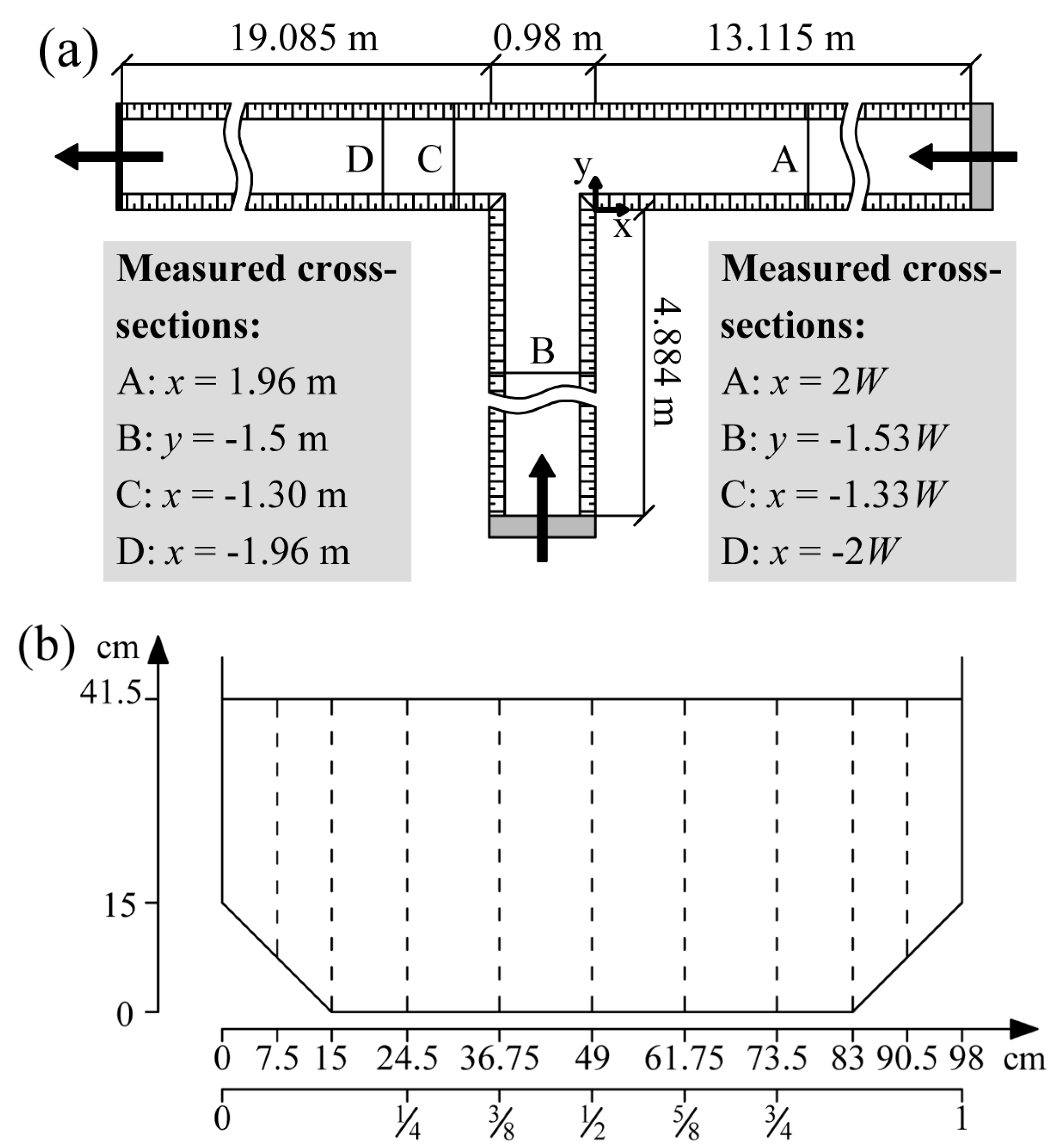
Experiments are carried out in an existing 90° angle confluence flume with concrete walls. All the channels of the confluence are horizontal, concordant and have a chamfered rectangular section with a width W of 0.98 m, as depicted in Figure 2. Note that the chamfered cross-section is typical for rectangular sections made with in situ cast concrete, where the chamfering is meant to simplify the removal of the formwork. While to the best of our knowledge no other laboratory studies used a chamfered section, movable bed studies and field sites exhibit a wide range of cross-sections, which may show some similitude to a chamfered rectangular section. At the upstream boundaries, flow straightening screens are installed, so that a relatively uniform and stabilized flow is retrieved. The downstream water level (h = 0.415m) is controlled by means of a weir.

Figure 2. (a) Top view of the laboratory experiment; (b) Cross-section of channels.

Figure 2. (a) Top view of the laboratory experiment; (b) Cross-section of channels.

Of the two discharge ratios that are investigated experimentally, one (q = 0.25) is inside the range covered in literature ($0.1 \lesssim q \lesssim 0.9$), and one (q = 0.05) is deliberately chosen outside that range. In both experiments, the total downstream discharge Q_d is kept constant at a value of 40 L/s. In addition, the downstream water level is constant, and hence the downstream Froude number Fr_d is constant as well, equalling 0.05. Although the Froude number is small compared to other laboratory experiments (see overview in [12]), the current value is in the typical range for lowland rivers [19]. As expected for such low subcritical flows, measurements by means of ultrasonic water level sensors show that the variation in the water level over the confluence is negligible. The Reynolds number based on the hydraulic radius equals 9.8 × 10⁴.

Flow velocity at the water surface is measured by means of surface particle tracking velocimetry (PTV). The PTV technique is conducted by seeding the water surface with floating polypropylene tracers, which are coated and have a maximum size of about 5 mm. A 1920 × 1080 camera takes images of the tracer at a frequency of 30 Hz. In processing, these images are rectified by means of the software FIJI, and the individual particle paths are tracked at a rate of 10 Hz. Eventually, the useful image recordings have a length of about 3 min. By using the PTV technique, it is possible to measure the surface velocities with a very high spatial resolution, providing better results than the particle image velocimetry technique adopted in preliminary experiments reported in [12].

Complementary to the measurements of surface velocity, Acoustic Doppler Velocimetry (ADV) measurements are performed in a selection of cross-sections, as indicated in Figure 2. The ADV equipment, namely a Nortek Vectrino II, is a profiling instrument able to measure profiles of 3 cm, but the sweet spot offers the largest accuracy over the profile. The vertical height of the measurement cell equals 2 mm, and only measurements with a sufficiently high signal-to-noise ratio and correlation larger than 80% are retained. The selected despiking algorithm is that of Goring & Nikora [20], as discussed by Wahl [21]. Following experience from preliminary measurements, the measuring time of 2 min is sufficient to capture the mean velocity.

Additionally, the total measurement error of ADV is estimated by performing different measurements at the same point, while resetting the incoming discharges in the confluence flume and repositioning the instrument at the given measurement point. This verification is done in the upstream channel, and results in a standard deviation of the mean of about 0.001 m/s in the longitudinal direction and 0.002 m/s in the lateral and vertical directions. It should be mentioned that the aforementioned uncertainties are lower bounds for the ones in the confluence area, where complex 3D flows are present. Especially near strong local gradients, a small positioning error will result in a relatively large velocity error, i.e., measurement error is inseparable from measurement location. As a check on both measurements techniques, PTV measurements are compared to ADV results close to the water surface, showing a good agreement.

The adopted coordinate system is presented in Figure 2. Since the z-axis, originating at the bed, points upwards, a right-handed system is established. In this work, the instantaneous velocity components in the longitudinal (x), lateral (y) and vertical (z) direction are denoted as u, v and w, respectively, whereas the corresponding time-averaged velocity components are denoted as $\overline{u}$, $\overline{v}$ and $\overline{w}$, respectively. As a length scale and velocity scale, the width of the channels W (= 0.98 m) and the bulk velocity in the downstream channel U_d (= 0.104 m·s⁻¹), respectively, are utilized. The (downstream) water depth h (= 0.415 m) is also used as a length scale in the vertical direction, when appropriate.

3. Numerical Model Simulations

3.1. Model Description

In order to simulate the 3D complex flow patterns in a confluence, several numerical modeling strategies are available, based on different assumptions; hence governed by different equations, and requiring different amounts of computational effort. Since the research objectives include the study of dynamic flow features like coherent structures, intermittent flow patterns and upwelling of the flow, use will be made of 3D large-eddy simulations (LESs), which require more computer resources than RANS models but are more appropriate to resolve the aforementioned (time-dependent) features. The theory behind this type of simulation has been explained extensively in literature [22,23,24]. Briefly, the Navier-Stokes equations are spatially filtered, such that smallest scales (eddies) are removed. Their influence is modeled by a so-called sub-grid scale (SGS) model. The large eddies are retained and are resolved on a mesh in space and time, by solving a discretized version of the filtered equations. LESs have already been applied successfully to study confluence hydrodynamics (e.g., [13,16,17,25]).

The present simulations are run in the OpenFOAM suite (version 2.2.2, OpenFOAM foundation, London, UK), which is an open-source code for computational fluid dynamics. As an SGS model, the standard Smagorinsky model is selected, since this has successfully been applied to laboratory confluences [25], and sensitivity to modeling dissipation in the smallest scales is small compared with the influence of boundary conditions and mesh resolution [26,27].

In order to reduce the required computational efforts, and to simulate rough walls more easily, the near-wall boundary layer is not fully resolved (as in [13]), neither is a near-wall RANS model applied (as in [16,17]) but it is simply modeled by means of a wall function (as in [25]). The wall function that was implemented by the authors in OpenFOAM discerns three sublayers of the turbulent boundary layer:

$$\{\begin{array}{c}\begin{array}{ccc}{v}^{+} = \frac{1}{\kappa } \ln \left({\text{z}}^{+}\right) + 5.5 + B& \mathrm{if}& z^{+} \ge 30\end{array}\\ \begin{array}{ccc}{v}^{+} = 2\frac{1}{\kappa }\ln \left(z^{+}\right) - 3.05 + B& \mathrm{if}& 30 > z^{+} > 5\end{array}\\ \begin{array}{ccc}{v}^{+} = z^{+}& \mathrm{if}& z^{+} \le 5\end{array}\end{array}$$

(2)

where v⁺ and z⁺ are the wall coordinates; k is the von Karman constant and the parameter B accounts for the wall roughness [28]:

$$\{\begin{array}{c}\begin{array}{ccc}B = 0& \mathrm{if}& k_s^{+} < 2.25\end{array}\\ \begin{array}{ccc}B = \frac{1}{\kappa } \ln \left(\frac{k_s^{+} - 2.25}{87.75} + C k_s^{+}\right) \sin \left[0.4258 \left(\ln \left(k_s^{+}\right) - 0.811\right)\right] & \mathrm{if}& 2.25 \le k_s^{+} < 90\end{array} \\ \begin{array}{ccc}B = \frac{1}{\kappa } \ln \left(1 + C k_s^{+}\right)& \mathrm{if}& k_s^{+} \ge 90\end{array}\end{array}$$

(3)

where $k_s^{+}$ is the dimensionless roughness height and C is a tuning parameter (equal to 0.5). Although the assumptions underlying the wall function may not be valid in complex flows, the wall function, i.e., Equation (2) above, has been used successfully by van Balen et al. [26,29] in a mildly curved bend, (though with a more simple formulation for the wall roughness parameter B than Equation (3)). In the present work, the wall roughness height used in Equation (3) is set equal to 1 mm, which provides the best correspondence with the experiments in the confluence flume with the concrete walls. Roughness has indeed a significant impact on flow in a confluence [30].

For an LES, it is important that the incoming flow contains sufficient and correct turbulence scales [22,23,24]. Therefore, the inlet velocity field is copied from a section downstream of the inlet, onto which random fluctuations are imposed. This implementation resembles a precursor iteration, only with the precursor domain attached to the domain of interest. Such a situation is advantageous, since no additional memory storage is required. At the downstream boundary, convective boundary conditions are applied. In the present simulations, the free surface is modeled by means of a so-called rigid lid. This approach has been applied to many types of open channel flows, see e.g., [16,17,23,24,26,27,29], although more complex surface tracking methods are also in use [9,13,25,31]. However, because of the small Froude number in the present experiments, the rigid lid is certainly a valid approach, and preferable because of reduced computational efforts.

The mesh contains 4.2 million cells, with 106 × 37 cells in the lateral and vertical direction. All channels in the computational domain of the confluence are 5 m long, which might seem long for the inlet channels. However, recalling that this length includes the precursor simulation, it ensures fully developed inlet flow. The mesh is slightly coarsened towards the inlet and outlet boundaries, where the largest cell aspect ratios of the domain can be found, equaling 3. Discretization in space (finite volume) and time are second order accurate. The time-step in the LES equals 0.025 s (= 2.65 × 10⁻³ W/U_d). After about 7.5 flow through times (= 760 s = 80 W/U_d), collection of flow data started (t = 0), over an additional 16.5 flow through times (= 1640 s = 175 W/U_d).

Two simulations were performed corresponding to the two discharge ratios (q = 0.25 and q = 0.05) in the experiments. Additionally, the limiting case q = 0, i.e., all discharge coming from the tributary, was simulated in a third LES. The mesh remains the same for all the simulations, which aids the intercomparison of the results.

3.2. Verification of the Simulations

As a first step in the verification process, it is checked whether the dimensionless wall distance z⁺ is in an acceptable range for the use of a wall function. It is found that z⁺ is generally sufficiently high (20 to 45) to allow the use of a wall function (requiring $20 \le z^{+} \le 500$ [22,23,24]). However, in regions of very low velocity, e.g., still flow in the upstream channel in the case where q = 0, the use of a wall function introduces some inaccuracies [27], due to $z^{+}$ being lower than 20. However, to keep inaccuracies as small as possible, the adopted wall function includes the buffer layer and the laminar sublayer.

In a second step, the percentage of resolved turbulent kinetic energy is assessed, as advocated by Pope [32]. Practically, the unresolved sub-grid energy is estimated by employing the formulations of Coussement et al. [33]. In contrast to an LES where the full boundary layer is resolved, the main part of the turbulent kinetic energy in the cells close to the wall is modeled by the wall function. Accordingly, these cells will by definition match the criterion to a lesser extent. This explains why not all cells exhibit a resolution of minimum 80%, the threshold value advocated by Pope [32] (Figure 3a). Notably in the upstream channel at q = 0.25, the relatively low velocity causes the first cell to be in the buffer layer. Hence, much turbulent kinetic energy is modeled here, leading locally to a less resolved LES. At even lower velocity in the upstream channel (i.e., at decreasing q), the cells closest to the wall are located in the viscous sublayer (recall that all discharge ratios are simulated using the same mesh), so that the LES is more resolved (Figure 3a). Of the cells that resolve less than 80% turbulent energy in q = 0.25, 72% is located in the upstream channel (x > 0). This confirms that the region of interest, i.e., the confluence area (x < 0), is well resolved.

Comparison of the simulation results with a finer mesh (consisting of 4 times the aforementioned number of cells) did not result in significant differences; hence, it is concluded that the results from the adopted mesh are sufficiently mesh-independent.

Further verification includes determining the Kolmogorov time scale, and linking this to spectral density. For the point with coordinates (x = −1.33 W, y = 0.75 W, z = 0.95 h), the Kolmogorov scale equals about 1 s, which corresponds to the end of the −5/3 law in the spectrum, as is to be expected (Figure 3b). The upper axis of Figure 3b provides the number of cells associated with an eddy of a certain frequency (adopting a typical mesh width Δ of 0.01 m), indicating that the structures associated with the Kolmogorov time scale are about 10 cells large. This corresponds to rules of thumb regarding the minimum number of cells necessary to resolve an eddy (5 to 20 [22]; ≥ 6 [23]). Additionally, the −5/3 region is present over about an order of magnitude, affirming the LESs are sufficiently well resolved.

Figure 3. (a) Percentage of turbulent kinetic energy resolved in the simulations; (b) Spectral density of the turbulent kinetic energy at the point with coordinates (x = −1.33 W, y = 0.75 W, z = 0.95 h) at q = 0.25. The frequency associated with the Kolmogorov scale is indicated by a dotted line.

Figure 3. (a) Percentage of turbulent kinetic energy resolved in the simulations; (b) Spectral density of the turbulent kinetic energy at the point with coordinates (x = −1.33 W, y = 0.75 W, z = 0.95 h) at q = 0.25. The frequency associated with the Kolmogorov scale is indicated by a dotted line.

3.3. Validation of the Simulations

A comparison of the LES velocity results with the experimental ADV data (in the cross-sections x = −1.33 W and x = −2 W) generally exhibits a close correspondence (Figure 4). The velocity gradient over the shear layer of the separation zone might appear sharper in the numerical simulations, but this can be attributed to the linear interpolation of $\overline{u}$ between the measured verticals. Although the lateral and vertical velocity also show a good correspondence, a zone of reduced $\overline{v}$ and $\overline{w}$ is present near the top right in the case where q = 0.25 (Figure 4a,c), while the LESs predict a cell rotating in the clockwise direction. Nevertheless, the LESs correctly simulate that this cell changes direction in the q = 0.05 case (to be discussed in Section 4.2.4), see Figure 4e,f. This indicates that trends are correctly simulated. Finally, a comparison is also made between the PTV (surface) data and the LES (at a height of z = 0.9 h to avoid the influence of the rigid lid) in Figure 5. It should be mentioned that in zones of upwelling flow (see Figure 6 in the results section for a presentation of flow features), the PTV might be biased to record a reduced upwelling, as these zones are rapidly depleted of tracers. This explains some differences between the PTV and LES at the end of the separation zone, and in the zone of upwelling flow near the right bank in Figure 5d. However, the correspondence, both in the longitudinal and lateral direction, demonstrates the appropriateness of the rigid lid approximation, and confirms the reliability of the LES results over a wide range of the confluence area.

Compared with earlier simulations [34], the adopted wall function and inlet condition in this paper prove superior in modeling the experimental set-up.

Figure 4. Comparison of experimental measurements on the left and numerical results on the right, for the measured cross-sections. The color scale indicates the time-averaged longitudinal velocity, which is interpolated between the measured verticals for the ADV data, and arrows represent lateral and vertical velocity. The dotted line indicates $\overline{u}$ = 0, i.e., separates upstream and downstream flow. In the left figures, the measured locations are indicated with grey lines, and the arrows are located in the sweet spots. (a,b) q = 0.25, x = −1.33 W; (c,d) q = 0.25, x = −2 W; (e,f) q = 0.05, x = −1.33 W; (g,h) q = 0.05, x = −2 W.

Figure 4. Comparison of experimental measurements on the left and numerical results on the right, for the measured cross-sections. The color scale indicates the time-averaged longitudinal velocity, which is interpolated between the measured verticals for the ADV data, and arrows represent lateral and vertical velocity. The dotted line indicates $\overline{u}$ = 0, i.e., separates upstream and downstream flow. In the left figures, the measured locations are indicated with grey lines, and the arrows are located in the sweet spots. (a,b) q = 0.25, x = −1.33 W; (c,d) q = 0.25, x = −2 W; (e,f) q = 0.05, x = −1.33 W; (g,h) q = 0.05, x = −2 W.

Figure 5. Comparison of experimental measurements of the surface velocity (PTV) and the numerical predictions. (a) q = 0.25, experimental; (b) q = 0.25, LES; (c) q = 0.05, experimental; (d) q = 0.05, LES.

Figure 5. Comparison of experimental measurements of the surface velocity (PTV) and the numerical predictions. (a) q = 0.25, experimental; (b) q = 0.25, LES; (c) q = 0.05, experimental; (d) q = 0.05, LES.

Figure 6. Time-averaged flow patterns near the surface (z = 0.9 h). Arrows indicate the longitudinal and lateral velocity component, while the color represents the vertical velocity component. The location of the mixing interface and the extent of the separation zone are indicated by a line. (a) q = 0.25; (b) q = 0.05; (c) q = 0.

Figure 6. Time-averaged flow patterns near the surface (z = 0.9 h). Arrows indicate the longitudinal and lateral velocity component, while the color represents the vertical velocity component. The location of the mixing interface and the extent of the separation zone are indicated by a line. (a) q = 0.25; (b) q = 0.05; (c) q = 0.

4. Results

In Section 4.1, the flow features will be presented for the reference case characterized by a moderate discharge ratio q = 0.25, i.e., the case in which the tributary incoming flow rate Q_t is (only) 3 times larger than the upstream channel incoming flow rate Q_m (or U_tQ_t/U_mQ_m = 9). The changes in flow features at small discharge ratios will be presented in Section 4.2 for the cases with q = 0.05 (or Q_t/Q_m = 19 and U_tQ_t/U_mQ_m = 361) and q = 0 (or Q_t/Q_m → ∞ and U_tQ_t/U_mQ_m → ∞).

4.1. Reference Case with Moderate Discharge Ratio (q = 0.25)

To illustrate the flow patterns, Figure 6a presents a plot of the (time-averaged) velocity at a height of 1/10h below the surface (z = 0.9h). The arrows represent the velocity vector in the horizontal plane, while the color scale represents the vertical velocity component $\overline{w}$. For clarity, Figure 6a also presents the location of the mixing layer and the extent of the separation zone. These locations are determined as follows.

The mixing layer is determined by means of the streamline departing from the confluence apex, in the horizontal plane z = 0.9h (i.e., neglecting the vertical velocity component), since Mignot et al. [11] also used this starting point for a 2D streamline marking the mixing layer. The separation zone, which is present in the schematized sections when the tributary flow is sufficiently important, has been delineated in literature by different methodologies. For example, Best & Reid [35] used surface dye tracers and neutrally buoyant particles. Gurram et al. [6] measured the separation zone by means of dye injections. Finally, Shumate [8] utilized his three-dimensional velocity measurements. In this paper, the (time-averaged) velocity field is also utilized to determine the extent of the separation zone. To this end, the y-coordinate Y at which there is a net zero discharge is determined for a given cross-section (with coordinate x) and at a given elevation above the bed (with coordinate z):

$${\int }_0^Y\overline{u}(x, y, z) \text{d}y = 0$$

(4)

The time-averaged flow in the reference case q = 0.25 will now be presented. Briefly, the flow has all the well-known features of a confluence flow (Figure 1). At the upstream confluence corner, a stagnation zone is present. The streamlines, which start there, separate the tributary inflow from the upstream channel inflow. The merging of the two flows causes the upstream channel flow to deflect towards the right bank, as can be derived from the path of the streamline between the incoming flows. These streamlines actually delineate a shear layer (also called the mixing interface), i.e., a zone of strong momentum gradients in the direction normal to the flow [11]. The vertical velocity shows that the flow from the upstream channel dives near the mixing layer, while the tributary flow surfaces (due to a helicoidal cell, see Section 4.2.3).

At the downstream corner of the confluence, the tributary flow detaches from the wall, and a separation zone is formed. In the separation zone, the flow near the wall has typically an upstream oriented velocity component, i.e., recirculating flow is present. In the separation zone, the flow generally dives, because the entrainment by the tributary causes a decrease in water level [6,7,35]. However, near the left bank in the separation zone, upwelling flow is present. This is caused by flow intruding the separation zone, starting at the bed. As a consequence, the separation zone is smaller near the bed than at the top of the water column [8,11,12,13]. Preliminary numerical simulations have indicated that this upwelling is enhanced by the presence of the chamfers [34]. Next to the separation zone, the joining flow from the two merging channels is contracted. The disappearance of gradients, which is enforced by the flow contraction, fades the shear layer, though the two flows can still be discerned downstream by means of the vertical velocity. Eventually, the flow takes the full width of the downstream channel, though fully uniform flow is not yet achieved in the numerical model.

Thus, the time-averaged flow corresponds to the known flow patterns (Figure 1) according to the conceptual model proposed by [1]. Experiments in the well-known range $q \gtrsim 0.1$ have shown that the three-dimensionality of these features intensifies at decreasing q [6,7,8,13].

4.2. Cases with a Small Discharge Ratio (q = 0.05 and q = 0)

4.2.1. Confluence Area and Upstream Channel

When the discharge ratio decreases, i.e., less flow is coming from the upstream branch, the tributary flow is less deflected by the upstream channel. This can be illustrated by means of the average inflow angle $\alpha$ at the cross-section y = 0 with which the tributary flow enters the confluence:

$$\alpha = {\int }_A^{ }\mathrm{atan}( \overline{v} / -\overline{u} ) \text{d}A$$

(5)

The results show that the average inflow angle increases from $\alpha$ = 65° at q = 0.25 to $\alpha$ = 71° at q = 0. Note that this angle is less than the geometrical confluence angle $\text{θ}$ = 90°, as was also observed in other laboratory experiments [4,7]. As a consequence of both the increased tributary discharge and the increased inflow angle, the tributary flow protrudes further towards the opposing bank. This can be seen by observing the location of the mixing layer in Figure 6: the mixing layer shifts towards the upstream channel, as the inflow from the upstream channel decreases. When comparing the cases q = 0.25 and q = 0.05, and observing the position of the mixing layer, one can see that the tributary flow stretches to the opposing bank in the case q = 0.05. As is observed when looking at the vertical velocity, it is more correct to say that the tributary flow impinges on the opposing bank: near the right bank in the downstream channel, a zone of upwelling flow is present, which already starts in the confluence area. This is consistent with the preliminary findings of Schindfessel et al. [12], and is also found lower in the water column in the present simulations. For the q = 0 case, the velocity vectors on the x = −0.30 W line are even more orthogonal to the wall. Thus, the impinging is a new flow feature, absent at q = 0.25, but present at q = 0.05 and q = 0.

While the main part of the impinging flow is directed to the downstream channel, a part is pushed into the upstream channel. There, it drives a horizontal recirculating eddy (or gyre), which blocks the upstream channel incoming flow (Figure 6). Looking at the section x/W = 0, presented in Figure 7, clarifies the flow patterns at the interface between upstream channel and the confluence area. At q = 0.25, nearly all velocity is directed in the downstream direction, apart from some zones near the bottom. The highest longitudinal velocities are present near the right bank, while closer to the left bank (i.e., to the upstream confluence corner), the longitudinal velocity magnitude is lower. This corresponds to the known flow patterns (Figure 1 after the conceptual model proposed by Best [1]): near the upstream confluence angle, a zone of stagnating flow develops, while the flow from the upstream channel is directed to the right bank by the momentum coming from the tributary inflow.

Due to the appearance of a horizontal recirculating eddy at small discharge ratio, however, flow from the confluence area protrudes into the upstream channel (upstream oriented velocity $\overline{u}$ in Figure 6b,c). Where the highest downstream velocity was noted in the q = 0.25 case, the highest upstream velocity is now found. Therefore, the position of the fastest downstream flow is shifted to the other bank as the discharge ratio approaches zero. This rupture from the trend at more moderate discharge ratios is attributed to the appearance of the recirculating eddy, induced by the impinging flow. Note that lateral and vertical velocity components are negligible to the longitudinal component, i.e., the recirculating eddy is a horizontal flow feature. The eddy also reduces the stagnation zone, in the sense that at $q \le 0.05$, no region of substantially lower flow is present near the confluence apex (left bank in Figure 7).

Figure 7. Cross section at x/W = 0, looking downstream. Color scale represents the time-averaged downstream velocity $\overline{u}$. Arrows represent lateral and vertical velocity. The dotted line indicates $\overline{u}$ = 0, i.e., separates upstream and downstream flow; (a) q = 0.25; (b) q = 0.05; (c) q = 0.

Figure 7. Cross section at x/W = 0, looking downstream. Color scale represents the time-averaged downstream velocity $\overline{u}$. Arrows represent lateral and vertical velocity. The dotted line indicates $\overline{u}$ = 0, i.e., separates upstream and downstream flow; (a) q = 0.25; (b) q = 0.05; (c) q = 0.

To quantify the importance of the recirculating eddy, and its growth when the discharge ratio decreases, the total discharge Q_u through the section x/W = 0 (i.e., the last section of the upstream channel) is split into two parts: Q_u = Q_u,out + Q_u,in. The “outflow” discharge Q_u,out represents the surface integral of all flow velocities oriented from the upstream channel to the confluence, whereas Q_u,in denotes the surface integral of all flow velocities oriented from the confluence to the upstream channel.

Although the recirculating eddy appears first at q = 0.05, its influence cannot be seen in the discharge parameters (Table 1). At q = 0, however, when there is no discharge in the upstream channel, the recirculating eddy pumps a discharge in the upstream channel that is of similar strength as the flow of q = 0.05. Obviously, the outflow discharge equals the inflow discharge, as there is no net discharge in the upstream channel. Table 1 thus quantifies that the exchange of mass from the confluence area into the upstream channel starts to be significant when q < 0.05.

Table 1. Composition of the total discharge Q_u through the section x/W = 0, for different discharge ratios q.

q (−)	Qu (m³·s−1)	Qu,in (m³·s−1)	Qu,out (m³·s−1)
0.25	0.010	0.000	0.010
0.05	0.002	0.000	0.002
0	0.000	0.002	0.002

Table 1. Composition of the total discharge Q_u through the section x/W = 0, for different discharge ratios q.

q (−)	Qu (m³·s−1)	Qu,in (m³·s−1)	Qu,out (m³·s−1)
0.25	0.010	0.000	0.010
0.05	0.002	0.000	0.002
0	0.000	0.002	0.002

4.2.2. Mixing Layer

The mixing layer, i.e., the shear surface between the incoming flows, is delineated (pragmatically) by the streamline starting at the confluence apex (see above). Compared with mixing layers in natural bathymetries [16,17], the mixing layer of the q = 0.25 case is relatively curved, as is typical for asymmetrical 90° confluences [11]. Due to the momentum inflow from the tributary, the mixing layer extends nearly to the opposing bank when entering the downstream channel (Figure 6). Only few vortices form in the mixing layer, and their strength is considerably smaller than the Kelvin-Helmholtz vortices that can be found in the separation zone (not shown). This may be attributed to the curvature of the mixing layer [36]. In the cases with dominant tributary flow, the increased flow from the tributary pushes the mixing layer towards the upstream channel, leading to a less curved mixing layer. When calculating the velocity gradient over the mixing layer, it is observed that the initial gradient is significantly higher at q = 0 compared with q = 0.25 (not shown). This is not only attributed to the larger velocity difference between the incoming channels, which is an obvious consequence of a smaller discharge ratio, but also to a decrease in the extent of the stagnation zone. The stagnation zone is not only reduced on the tributary side by the tributary’s increased discharge, but also on the upstream channel side, by the recirculating eddy.

4.2.3. Separation Zone

The maximum width and length of the separation zone, determined as explained previously, are shown in Table 2 together with the predictions based upon Best & Reid [35]. The widths compare reasonably well with the regression line, yet the length of the separation zone is consistently smaller. This can be explained by the chamfered rectangular section in this research, in contrast to the rectangular section of Best & Reid [35], as the chamfers aid the vertical flow of high momentum fluid from the bottom to the top of the separation zone, effectively decreasing the length [34].

As the tributary discharge increases, the velocity difference between tributary and separation zone increases as well. Since the velocity difference is the driving force in a shear layer, the shear in the separation zone strengthens with smaller q, resulting in a higher turbulent kinetic energy (TKE) (Figure 8). Not only is the absolute value of the TKE in the shear layer larger at smaller q, the region over which high TKE values are found is also larger (notably in the downstream direction). Note that the maximum TKE is not localized on the limit of the separation zone as defined in this work, but is slightly shifted to the side of the separation zone.

Figure 8. Turbulent kinetic energy (TKE) near the surface (z = 0.9 h). The location of the mixing interface, the velocity gradient between impinging and non-impinging flow and the extent of the separation zone are indicated by a line. (a) q = 0.25; (b) q = 0.05; (c) q = 0.

Figure 8. Turbulent kinetic energy (TKE) near the surface (z = 0.9 h). The location of the mixing interface, the velocity gradient between impinging and non-impinging flow and the extent of the separation zone are indicated by a line. (a) q = 0.25; (b) q = 0.05; (c) q = 0.

Table 2. Dimensions of the separation zone (z = 0.9 h).

	width/ W (−)		length/ W (-)
q (-)	Present Work	Best & Reid [34]	Present Work	Best & Reid [34]
0.25	0.50	0.45	1.40	2.29
0.05	0.55	0.50	1.25	2.53
0	0.55	0.51	1.35	2.59

Table 2. Dimensions of the separation zone (z = 0.9 h).

	width/ W (−)		length/ W (-)
q (-)	Present Work	Best & Reid [34]	Present Work	Best & Reid [34]
0.25	0.50	0.45	1.40	2.29
0.05	0.55	0.50	1.25	2.53
0	0.55	0.51	1.35	2.59

The largest TKE values can be found at about mid-depth, and are located closer to the wall, corresponding to the three-dimensional nature of the separation zone. Further, at lower depths, the TKE values in the separation zone and the region of high TKE values enlarge when the discharge ratio diminishes.

4.2.4. Contracted Flow and Flow Recovery Areas

The impinging flow that was indicated in Section 4.2.1 also has consequences for the flow patterns in the downstream channel. More specifically, the impinging causes the flow to surface near the right bank, as is well illustrated by the vertical velocity (Figure 6). In the q = 0.05 case, a large region of upwelling flow is noticed near the right bank ($y/W \approx 1$). Additionally, this zone is flanked by downward velocities in the contracting section. Such flow behavior was absent in the q = 0.25 case, where upwelling and diving were positioned differently, and were much weaker. The upwelling caused by impinging near the right bank in the q = 0 case is weaker than in the q = 0.25 case. Although this might be unexpected, decreased vertical velocities compared with q = 0.05 are already present lower in the water column at a more upstream position (near the opposing wall, around x = −0.5 W and z = 0.50 h, not shown). This decreased vertical velocity is associated with increased water levels (pressure on the rigid lid) in the case q = 0 versus q = 0.05: the increased water pressure at q = 0 counters the upward vertical motion, thus explaining the decreased upwelling noticed in Figure 5.

In order to clarify the secondary currents in the downstream channel, the streamwise-oriented vorticity (SOV) is employed. This parameter is calculated from the time-averaged velocity field and is defined as $\left(\nabla \times \overrightarrow{u}\right) · \overrightarrow{u} / \left|\right|\overrightarrow{u}\left|\right|$, whence it follows that it differs by a factor of $2\left|\right|\overrightarrow{u}\left|\right|$ from the helicity [37]. Using this parameter, Figure 9 shows the helicoidal cells in the section x = −1.33 W, revealing that there are three regions of augmented SOV. First, the shear layer between the separation zone and the contracted flow exhibits elevated values of SOV. However, the velocity gradients present in this layer create vorticity, but are not indicative of a helicoidal cell. Second, near the bottom (z < 0.05 W), a small clockwise-rotating cell is present (positive value of SOV), having its center around y = 0.40 W. It transports fluid from the contracted flow, having high velocity, to the separation zone, corresponding to the upwelling flow discerned before (Figure 6). Note that this intrusion of high velocity fluid dissolves the separation zone (indicated by a dotted line in Figure 9) from below. At a smaller discharge ratio, this bottom cell increases in strength, causing more upwelling in the separation zone. Both the presence and the increased strength at smaller q are in correspondence with the experiments (Figure 4). Third, near the right bank, one or more helicoidal cells are present. At q = 0.25, one clockwise cell is clearly present near the surface, with a counterclockwise cell beneath it. At the smaller q, only a single counter-clockwise cell remains, located near the surface. Consequently, lateral surface velocities near the right bank have a changed sign, being the result of the impinging flow. This is a very noticeable change of small discharge ratios. Although the third cell in q = 0.25 is not clearly visible in the experimental results, the cell of q = 0.05 is definitely present in the experiments (Figure 4), confirming that the LES predicts the effect of diminishing q correctly.

Figure 9. Cross section at x = −1.33 W, looking downstream. Color scale represents the streamwise-oriented vorticity of the mean flow. Arrows represent time-averaged lateral and vertical velocity. The dotted line indicates $\overline{u} = 0$, i.e., separates upstream and downstream flow; (a) q = 0.25; (b) q = 0.05; (c) q = 0.

Figure 9. Cross section at x = −1.33 W, looking downstream. Color scale represents the streamwise-oriented vorticity of the mean flow. Arrows represent time-averaged lateral and vertical velocity. The dotted line indicates $\overline{u} = 0$, i.e., separates upstream and downstream flow; (a) q = 0.25; (b) q = 0.05; (c) q = 0.

In order to characterize the recovery towards uniform flow in the downstream channel, a momentum coefficient $\beta$ is defined:

$$\beta = \frac{{{\displaystyle \int }}_A {\overline{u}}^2 \text{d}A}{Q_d U_d}$$

(6)

For a fully uniform flow β = 1, while the more non-uniform the velocity distribution is over the cross-section, the more β exceeds the unit value. Figure 10 presents the stated momentum coefficient, based on a selection of cross-sections. From comparing q = 0.25 and q = 0.05, it follows that at all longitudinal positions, a decreasing discharge ratio corresponds to an increasing non-uniformity. This is consistent with the increasing width of the separation zone (see above), which is the primary source of non-uniformity. However, at a discharge ratio equal to 0, the momentum coefficient levels out, i.e., at some longitudinal positions it is marginally higher than in case q = 0.05, while at other positions it is slightly lower.

Figure 10. Momentum coefficient $\beta$ of mean flow, characterizing the non-uniformity of the velocity distribution at different sections, as a function of the discharge ratio.

Figure 10. Momentum coefficient $\beta$ of mean flow, characterizing the non-uniformity of the velocity distribution at different sections, as a function of the discharge ratio.

Additionally, the results of section x = −4 W show that the recovery to uniform flow takes a longer distance, if the discharge ratio is smaller, notwithstanding the larger cross-sectional velocities when q diminishes. This finding can also be noted in Figure 6.

4.2.5. Turbulent Kinetic Energy

The increased initial velocity gradient increases the TKE in the mixing layer (Figure 8), and causes vortices in the mixing layer to be slightly stronger when tributary flow is dominant and to be less dissipated than in the reference case. In all cases, a zone of elevated TKE originates in the mixing later, as was observed in literature [11,16,17], but in the cases q = 0.05 and q = 0, the TKE significantly increases in value when it reaches the opposing bank. At mid-depth, the highest TKE levels are found in the mixing layer and near the opposing bank, while the contracted flow has less elevated levels of TKE (not shown). Closer to the surface, however, the larger TKE values are found in the flow contraction (Figure 8). Additionally, a velocity difference in the direction normal to the streamwise velocity is present in the time-averaged velocity field, indicated in Figure 8 as a distinct shear interface. This velocity difference can, to some extent, also be seen in the velocity plots of Figure 6. From Figure 9, on the other hand, it can be discerned that this shear layer is localized where impinging flow and non-impinging flow meet, i.e., large gradients in lateral velocity are present there. Although flow contraction is known to decrease velocity gradients, the velocity difference remains relatively constant when moving downstream, corresponding to the still important upwelling flow. The (three-dimensional) interface, where impinged flow meets with non-impinged flow, will lead to stronger fluctuations of the local velocity, and can thus explain the elevated levels of TKE in that region.

4.2.6. Intermittent Flow Patterns and Implications for Time-Averaged Results

In the laboratory experiments, was noticed that flow near the right bank exhibits a larger standard deviation in the case where q = 0.05 versus q = 0.25 [12]. In addition, it was visually observed that lateral flow is sometimes directed towards the bank, while at other instances in time, it is directed away from the bank. The change in sign of the lateral velocity seems to occur with a certain intermittency, as indicated by long ADV measurements at the point with coordinates (x = −1.33 W, y = 0.75 W, z = 0.95 h) indicated in Figure 11.

Figure 11. Time series of lateral velocity v at the point with coordinates (x = −1.33 W, y = 0.75 W, z = 0.95 h), in the experiment (ADV) and in the LES. (a) q = 0.25; (b) q = 0.05; (c) q = 0.

Figure 11. Time series of lateral velocity v at the point with coordinates (x = −1.33 W, y = 0.75 W, z = 0.95 h), in the experiment (ADV) and in the LES. (a) q = 0.25; (b) q = 0.05; (c) q = 0.

At this point, the numerical simulations of case q = 0.25 seem to match closely to the experimental values, as is visible both from the time-series as well as from a probability density function (Figure 11a and Figure 12). For the case q = 0.05, the experimental and numerical probability density functions match less well, though similar intermittent patterns in velocity direction are observed, having similar amplitudes (Figure 11b). Although there is an acceptable agreement between the measured and simulated mean velocity at this point, the period of these events seems to be much longer in the simulations than in the experiment. However, as the simulation exhibits intermittency having a similar amplitude, the numerical results can be used to further elucidate this phenomenon.

Figure 12. Probability density functions of the time series of lateral velocity $v$ shown in Figure 11, both for the experiment (ADV) and for the LES.

Figure 12. Probability density functions of the time series of lateral velocity $v$ shown in Figure 11, both for the experiment (ADV) and for the LES.

Figure 13 presents instantaneous streamlines at two instances in time, representing the extreme patterns within the range for the case q = 0.05, and Figure 14 shows the cross-section x = −1.33 W at these instances. In the flow patterns that are present most of the time, the tributary flow impinging on the opposing bank is located near the top of the water column, and is reflected towards the bottom of the downstream channel (Figure 13a and Figure 14a). The flow patterns associated with the upwelling event, however, are substantially different. The streamlines illustrate that the impinged flow moves upwards, i.e., strong upwelling is present, forming a strong helicoidal cell. The helicoidal cell is also discernible in the downstream channel (Figure 14b), explaining the negative v component in the time series (Figure 11b). Also note that the tributary flow reaching the opposing bank, i.e., the flow that impinges, is located rather low in the water column compared with the flow patterns that are present most of the time in the LES.

Figure 13. Instantaneous streamlines when q = 0.05, starting at x = −0.20W in the tributary channel, at (a) t = 540 s; (b) t = 740 s. Color scale indicates the vertical height at which the streamline is located. Red arrows indicate flow direction.

Figure 13. Instantaneous streamlines when q = 0.05, starting at x = −0.20W in the tributary channel, at (a) t = 540 s; (b) t = 740 s. Color scale indicates the vertical height at which the streamline is located. Red arrows indicate flow direction.

Figure 14. Instantaneous velocity in the section x = −1.33 W when q = 0.05, looking downstream, at (a) t = 540 s; (b) t = 740 s. Color scale indicates longitudinal velocity u, while arrows show the lateral and vertical velocity.

Figure 14. Instantaneous velocity in the section x = −1.33 W when q = 0.05, looking downstream, at (a) t = 540 s; (b) t = 740 s. Color scale indicates longitudinal velocity u, while arrows show the lateral and vertical velocity.

It is emphasized that such time dependent changes are also noted in the experiment, discernible by the two peaks in the histogram of Figure 12, indicated by the full green arrows. Changing surface velocity near the right bank was also observed visually by means of the PTV tracers. Notwithstanding that the LESs show larger periods, some similar events of high negative v are present (dotted green arrows in Figure 12). Although the probability density function accentuates the difference between the experiment and LES, the limb of the numerical histogram in the negative v is clearly non-zero.

For q = 0, similar intermittent shifts in velocities are noted (orange arrows in Figure 12), yet with seemingly larger intervals. In addition, the velocity amplitude is slightly larger. The instantaneous flow patterns of the modes resemble those of Figure 14, indicating a similar origin. Again, the position where the tributary impinges on the opposing bank seems to be associated with the intermittency.

The intermittent flow features that are observed trigger the question whether the aforementioned time-averaged flow was recorded over a sufficiently long period to be representative, even when the number of flow-through times seems acceptable. To assess this question, the time evolution of the time-averaged velocity is investigated. A good example is the q = 0 case: the difference in time-average velocity between 0 to 600 s and 0 to 1000 s is representative for the effect of the short but strong changes in flow patterns. Comparing these values in the horizontal plane, z = 0.90h indicates that that the time-averages change only 0.006 m/s on average. Similar conclusions can be drawn when comparing time-averaged values at 900 s and 1800 s in the case where q = 0.05. Consequently, these results underline that the time-averaged flow fields presented before are representative, despite the fact that they contain a limited number of upwelling events. Although this shows that the simulation time was sufficiently long, it should be noted that the presence of the helicoidal cell near the right bank (Figure 9) in the time-averaged velocity field can mainly be attributed to the upwelling event.

5. Discussion

Multiple authors have argued that the three-dimensional nature of the flow tends to intensify when the discharge ratio decreases (e.g., [6,7,8,13]). This trend is certainly confirmed by the present results, but moreover, some characteristic features of small discharge ratios are observed.

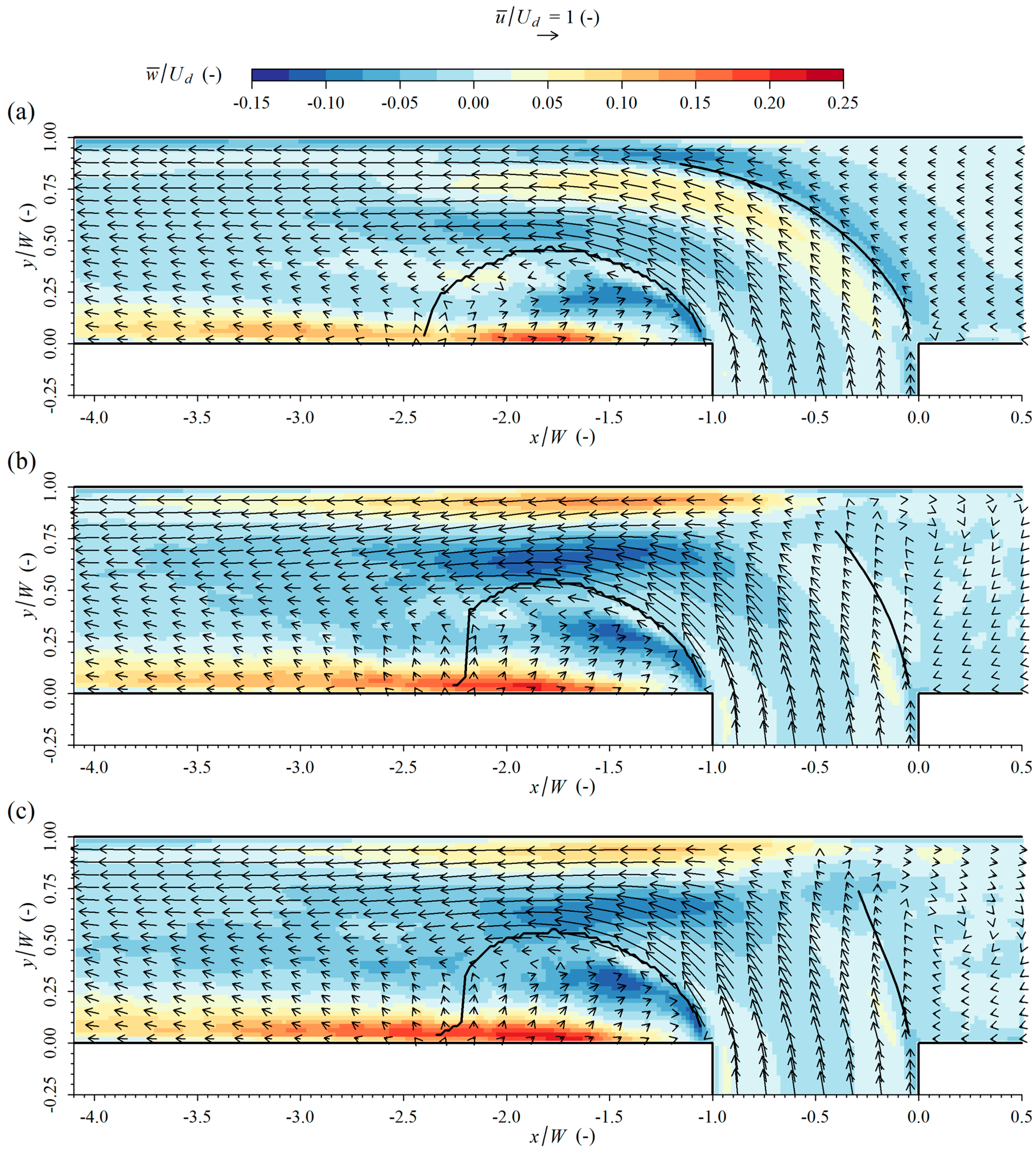
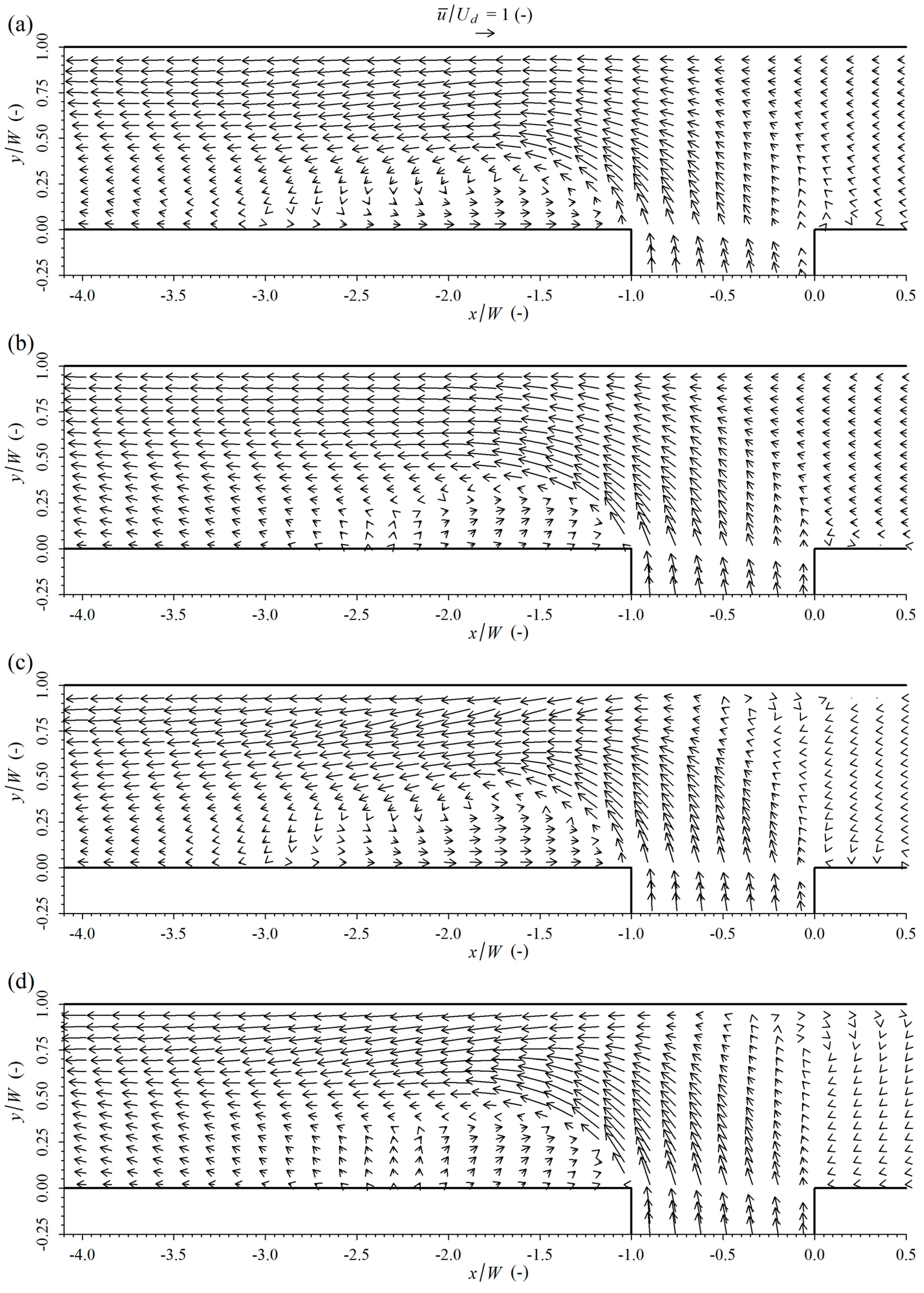
The most important novel feature of confluence flow at a small discharge ratio (i.e., when the contribution of the tributary is sufficiently dominant), is that the tributary flow impinges on the opposing bank. Although it is obvious to focus on the flow in the downstream channel, this research indicates that the presence of a recirculating eddy in the upstream channel, induced by the impinging flow, cannot be neglected. From Figure 6 it follows that the recirculating eddy gains a lot of strength between q = 0.05 and q = 0, indicating the aforementioned effects will be weak when q > 0.05. This might explain why a recirculating eddy was not discerned in Shumate’s [8] experiments at q = 0.083. One of the consequences of the recirculating eddy is that it effectively reduces the stagnation zone on the upstream channel side. Additionally, the stagnation zone is reduced on the tributary side when q diminishes, simply because more momentum is present. This was noticed by means of the average inflow angle $\alpha$, which decreases with decreasing q, i.e., the tributary inflow at y = 0 is less deflected. The observed inflow angle in the present simulations compares well with other studies, certainly when accounting for the much higher spatial resolution in LES compared with experiments: Hsu et al. [7] found an average angle of $\alpha$ = 75° at q = 0.1 and Hager [4] found $\alpha$ = 73° at q = 0. As the stagnation zone is thus reduced on both sides of the confluence apex, the stagnation point (i.e., where the streamline dividing the incoming flows starts [38]) will not shift as much to the confluence side as expected from analytical considerations [38]. A possible consequence of the recirculating eddy is that the exchange of solutes between the confluence area and the upstream channel may drastically change for discharge ratios smaller than 0.05. In these situations, sedimentation in the center of the upstream channel may be expected. Bergeron & Roy [39] for example, noted the accumulation of gravel at the entrance of the upstream channel after the break of an ice jam in the tributary. Although the gravel bar probably originates from the period during which the tributary channel was jammed (causing less transport capacity at the confluence), the accumulation could have been reinforced during the period of small discharge ratio when the ice jam broke [39].

In the downstream channel, the separation zone is highly three-dimensional; hence, it is difficult to characterize its width or length in one number [6,8,9,10]. Nevertheless, the separation zone gradually widens at the surface when the discharge ratio decreases, closely corresponding to the logarithmic regression provided by Best & Reid [35], even when the discharge ratio is outside their experimental range. The determination of the length of the separation zone suffers from the presence of upwelling flow near the end of the separation zone [8]. The upwelling flow prevents the separated flow from reattaching to the bank, an issue that is enhanced by the chamfered section [34]. This might explain why the length of the separation zone does not match with the results of Best & Reid [35]. Moreover, in field-based research, it was found that flow separation is sometimes absent. The flow separation might be suppressed by the gentle curvature of natural confluence corners, or by improved flow alignment introduced by the bathymetry [40,41,42]. Additionally, sediment can easily accumulate in the separation zone, inhibiting reverse flow [1].

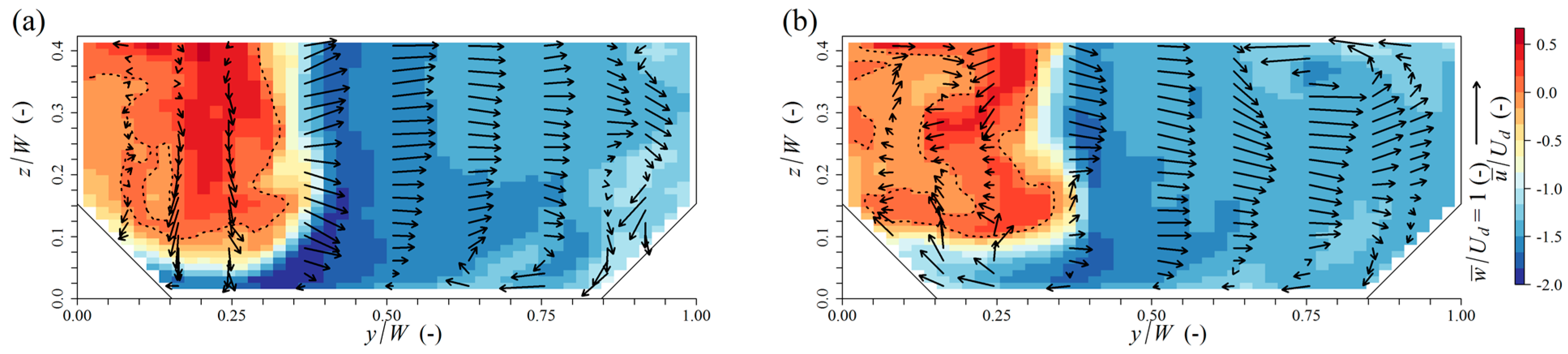
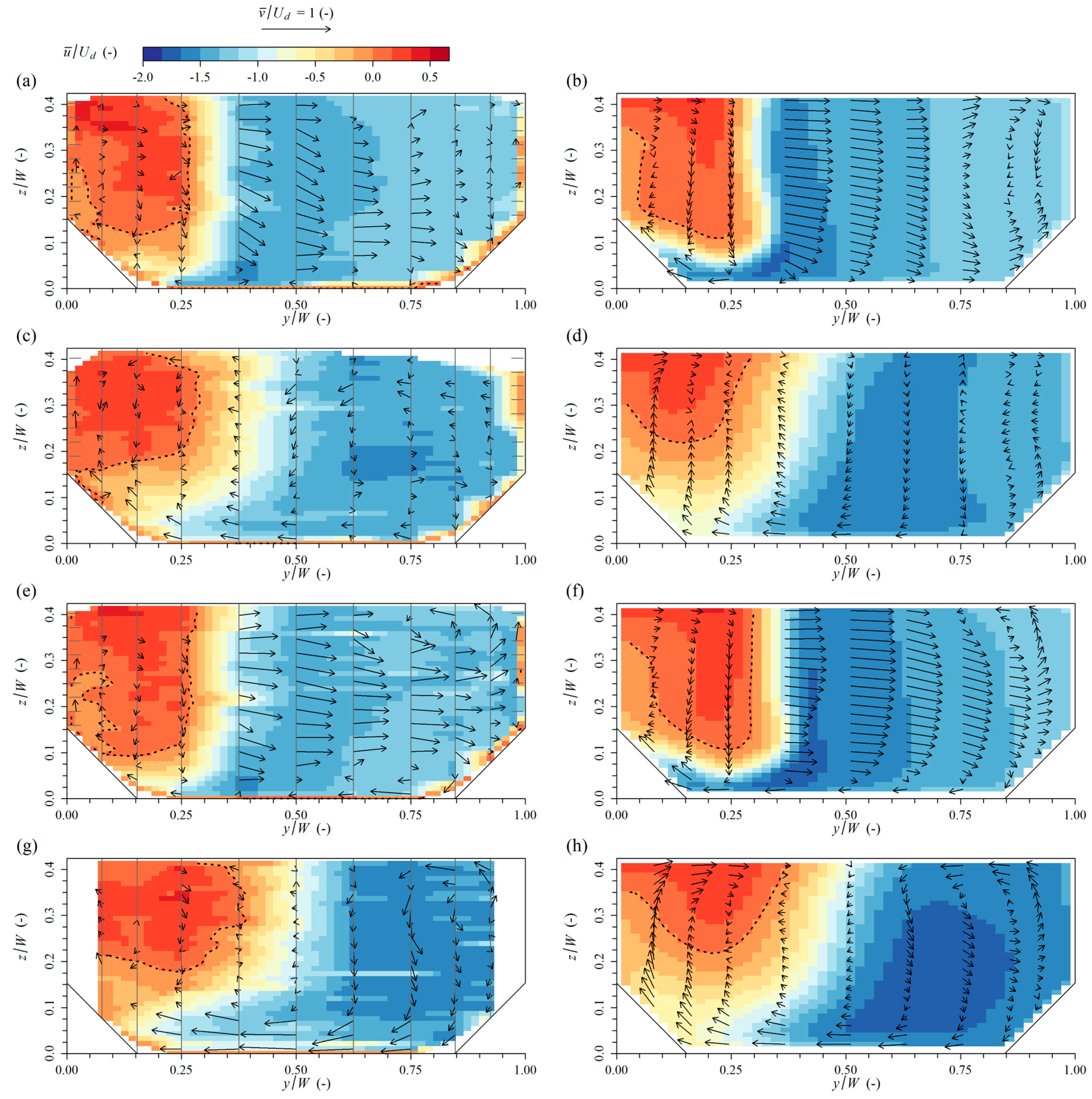
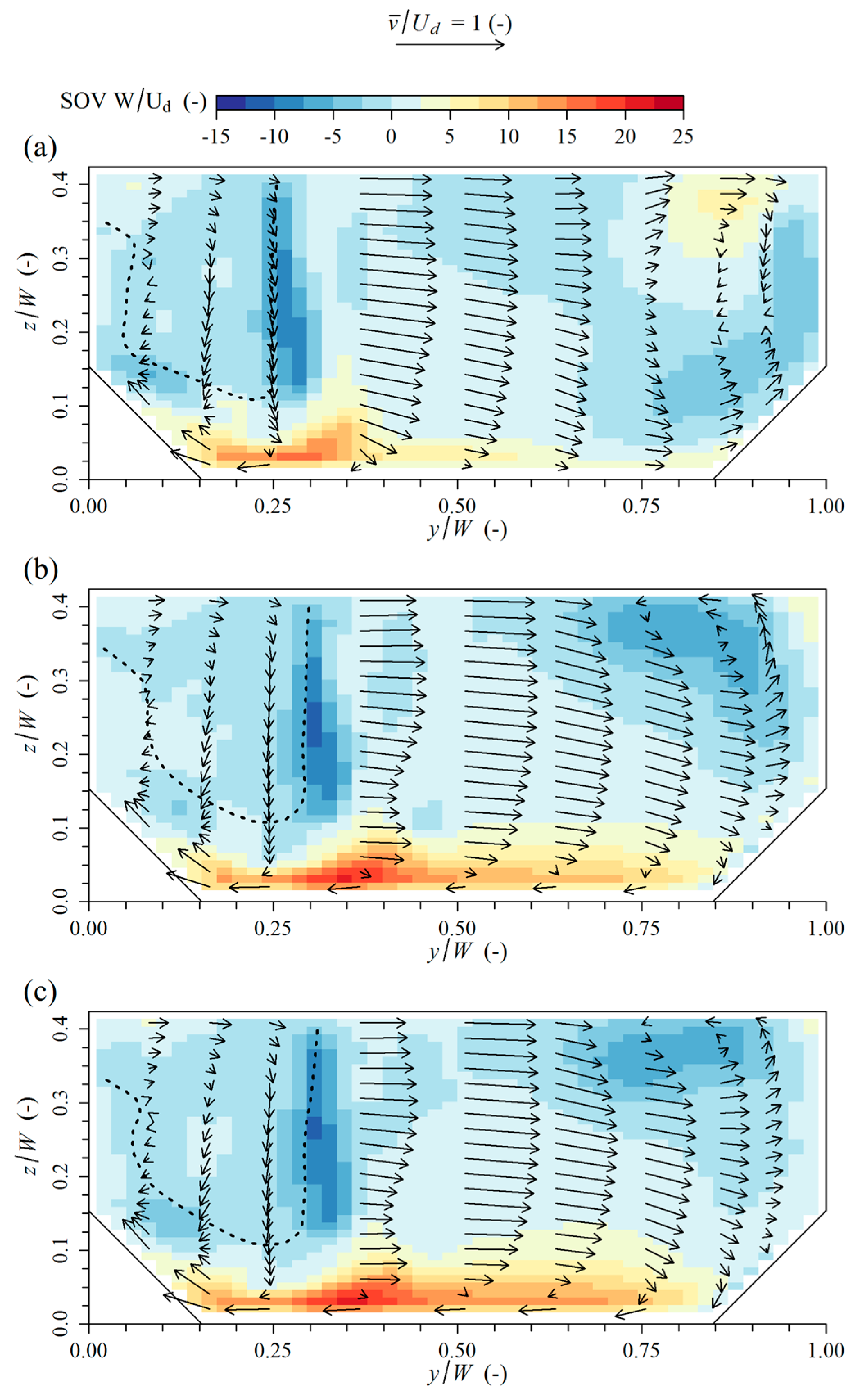
The secondary currents in the case where q = 0.25 show dissimilarities in comparison to those in the case of rectangular sections with similar width-to-depth ratio yet different Froude numbers, where one strong clockwise rotating cell is present [8,9,10,31]. The current simulations do show a clockwise cell, but it is located close to the bottom. Since impinging flow at a small discharge ratio causes important changes in secondary currents, similar changes can be expected in rectangular sections, though this statement is not verified in this work.

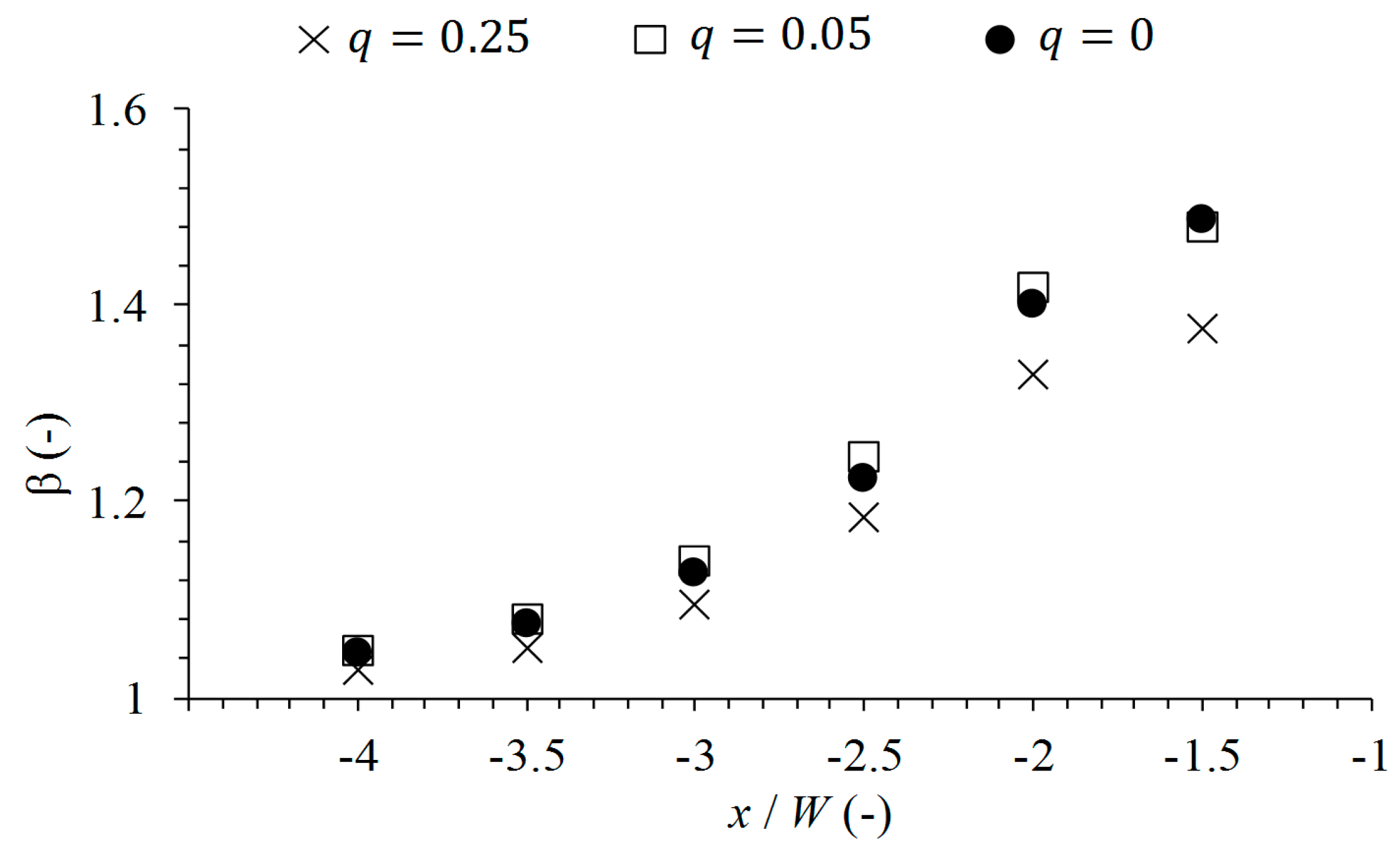
By means of a momentum coefficient β, it is also shown that the cross-sectional non-uniformity of the velocity distribution in the downstream channel increases when q decreases. However, only a slight change of β is noted when comparing q = 0.05 and q = 0. A comparison between the present values and literature is not easy, as Hsu et al. [7] defined a momentum coefficient $\beta$ in the function of the flow in the contracted section (excluding the separation zone), and the smallest discharge ratio measured by Ramamurthy et al. [5] equaled q = 0.40. Despite this, it can be concluded based on the current finding that the curve fit of Hsu et al. [7], stating that the momentum coefficient (of the contracted section) is inversely proportional to q, when $0.1 \lesssim q \lesssim 0.9$, is not valid for very small q; the momentum coefficient does not become infinitely large when q becomes extremely small—In contrast, it only changes marginally between q = 0.05 and q = 0. The curve proposed by Ramamurthy et al. [5] for high Froude numbers, i.e., a quadratic curve stabilizing at small q, seems to be more qualitatively correct. The flow patterns observed in the downstream channel can be tied to field-based research. For instance Rhoads et al. [15] noted that in the case of a dominant tributary flow, the scour hole migrates to the right bank of the downstream channel, and depositions take place near the inner bank. These findings are in line with the conceptual model of Best [1], and can be linked to the increased flow contraction at smaller q. Multiple studies also associate erosion of the outer bank with a small discharge ratio [14,15,39]. When making abstraction of differences in junction angle, bed geometry, etc., this corresponds to the tributary flow impinging on the opposing bank.

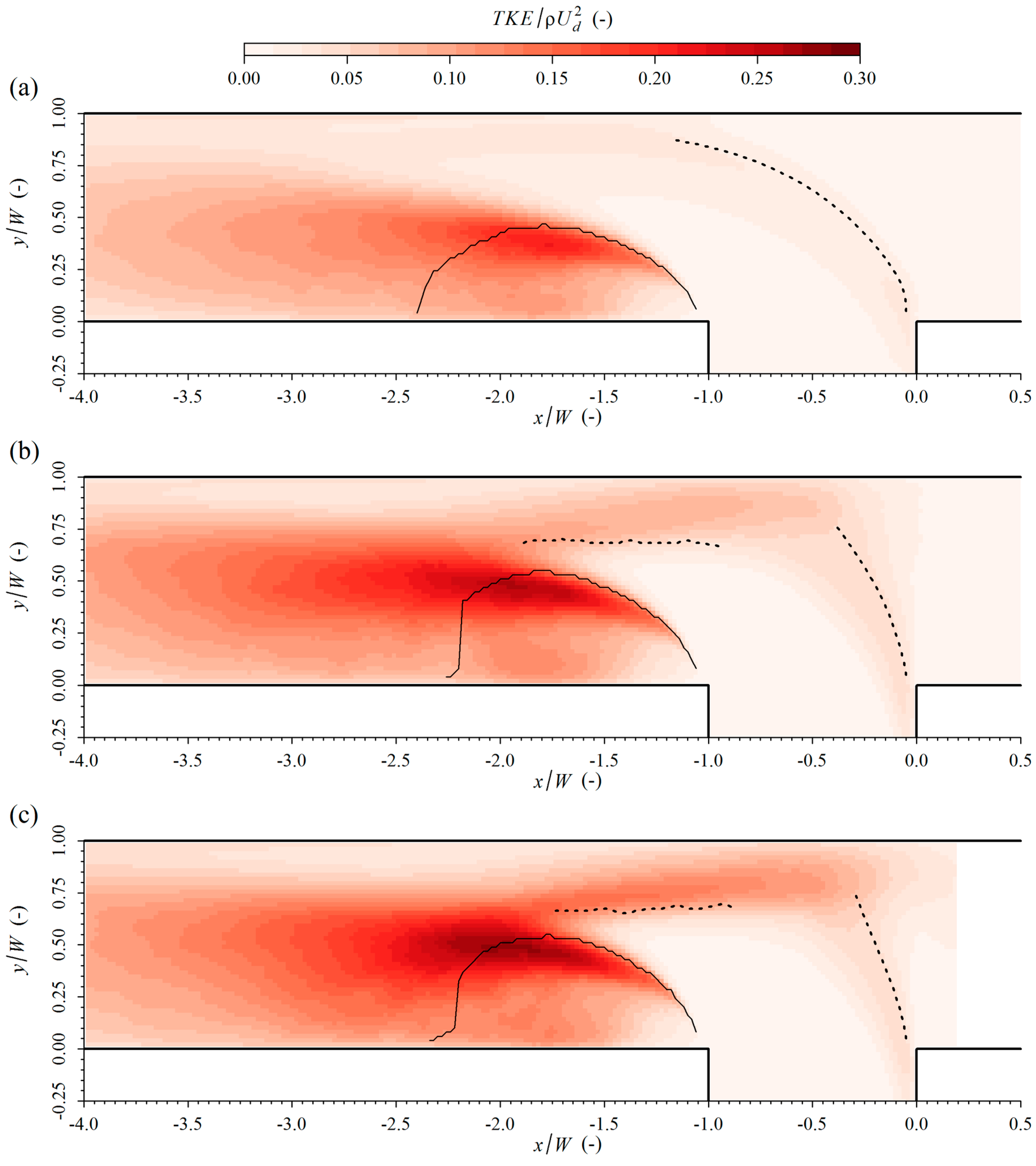
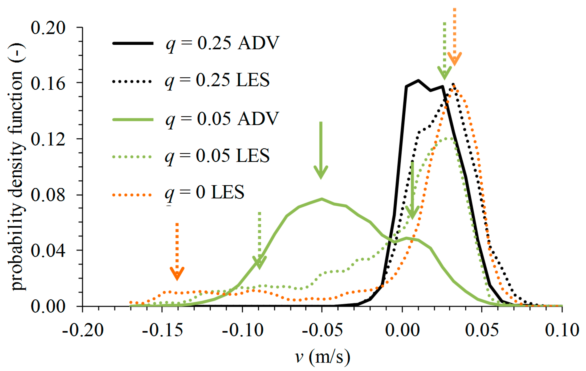
The velocity difference over the shear layer in the separation zone occurs at a moderate discharge ratio that is larger than that in the mixing layer. As a consequence, the largest TKE values are present in the separation zone. When q decreases, TKE increases in these shear layers. An important difference when tributary flow becomes dominant, is the appearance of a velocity gradient in the contracted section between the flow being impinged and reflected by the opposing wall, and the non-impinged flow. Furthermore, levels of TKE increase in the downstream channel as the discharge ratio decreases, which is consistent with the increased non-uniformity in this section. The former may introduce new paths of sediment transport, while the latter may induce stronger scour, in the case of movable bed confluences where bed-forming flows are associated with small q values.

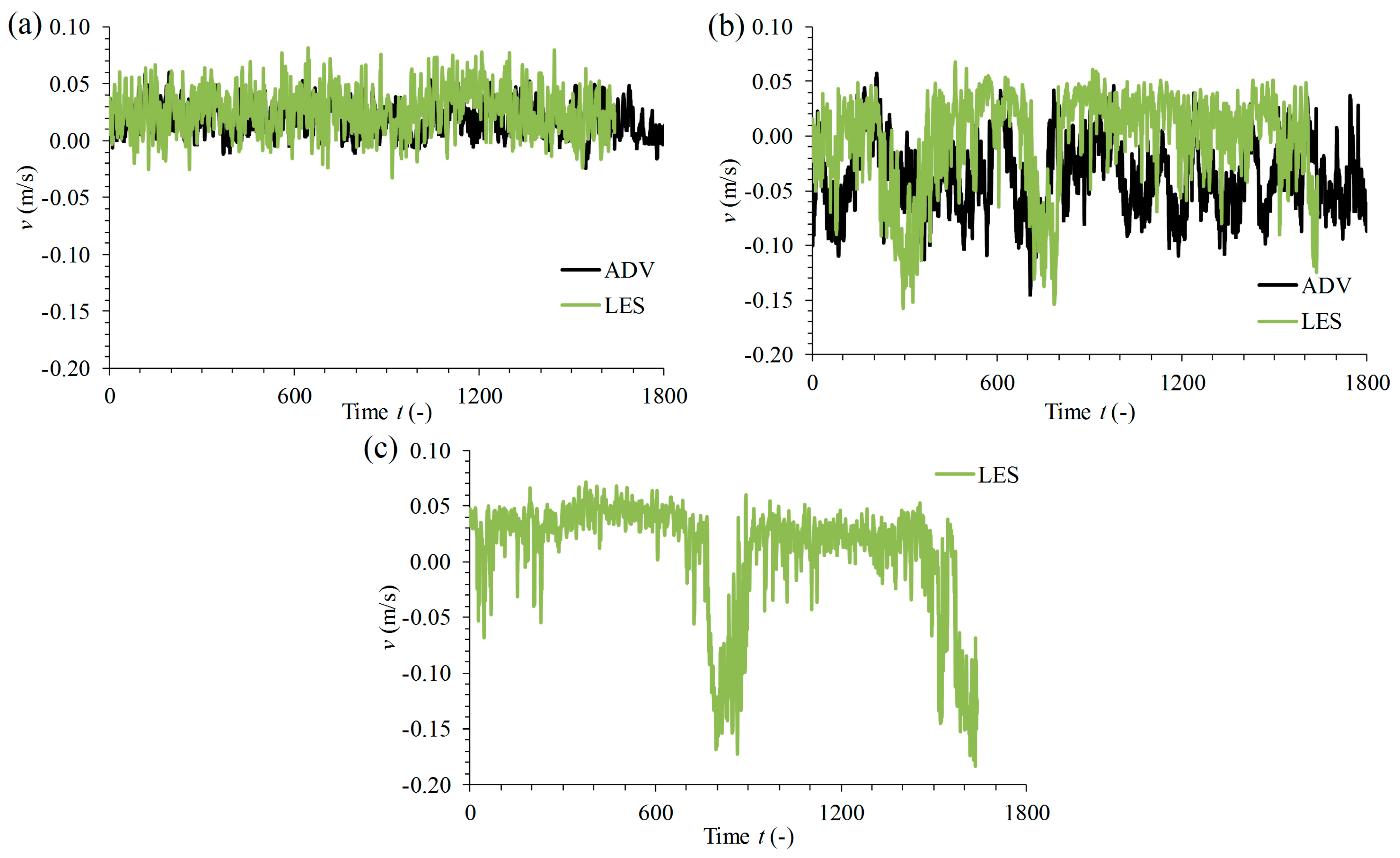
The intermittent flow patterns that were observed both in the experiment and in the LES have quite large intervals in time between two consecutive events. Instantaneous flow patterns show that these patterns are related to the position where the tributary flow impinges on the opposing wall, relating the intermittency to the discharge ratio. It is not yet clear whether the different vertical position of the impinging flow is a trigger for or a consequence of the intermittent flow patterns. Further research is needed to discover the cause of the intermittency. Knowledge of the cause might aid in improving the LESs, which simulate the amplitude correctly, but not the interval. Moreover, it seems that these intermittent flow patterns are dissimilar from those reported by Constantinescu et al. [16,17], where bimodal oscillations originate in helicoidal cells around the mixing layer. Further, in case of discordant beds, intermittent upwelling events are attributed to shear layer instabilities via streamwise eddies [25]. In the present research, however, the intermittent flow patterns are associated with the small discharge ratio and the impinging on the opposing bank.

6. Conclusions

This paper investigated the flow patterns in a subcritical junction using LESs, focusing on the case where the tributary provides the dominant part of the incoming discharge. Recalling the research questions stated in the introduction, one can conclude that increasingly dominant tributary flows, i.e., small discharge ratios, lead to:

• New features in the flow patterns induced by the impinging of the tributary flow on the opposing bank. In the upstream channel, a recirculating eddy develops, imposing rather significant changes on the incoming velocity. By changing the size of the stagnation zone, this also influences the mixing layer. In the downstream channel, the impinging flow causes stronger helicoidal cells, upwelling near the right bank and associated higher levels of TKE.
• Confirmation of some of the known trends in confluence literature, such as increased three-dimensionality of the flow, and increasing dimensions of the separation zone. However, the new flow features can be regarded as deviations from the known trends.
• Changes in the mixing layer, as the upstream channel inflow is influenced by the recirculating eddy. In addition, a new shear interface develops between the upwelling flow caused by impinging, and the non-impinging part of the tributary inflow follows a curved path to the downstream channel. The impinging flow enforces stronger helicoidal cells, though in the end, these do not result in faster flow recovery.
• Upwelling events of much stronger upwelling flow, having an intermittent character. They seem to be linked to the height at which the tributary impinges on the opposing wall, thus they are associated with the small discharge ratios.

Further research is needed to fully understand the origin of the intermittent upwelling phenomenon. Moreover, an open question remains whether the observed changes occur gradually between q = 0.25 and q = 0.05, or if there is a distinct discharge ratio at which the flow features alter. For $q \gtrsim 0.10$, no changes in flow patterns have been reported, while Shumate [8] identified reflection at q = 0.083. In the present research, it was found that the recirculating eddy in the upstream channel is weak at q = 0.05, but is fully developed at q = 0. Therefore, it can be speculated that a gradual transition exists between confluences with important tributary discharges and those with dominant tributary discharges.

The current research was conducted for relatively low Froude numbers, representative of lowland rivers. Validating the conclusions for higher Froude numbers remains to be performed. Similarly, it should be emphasized that the present research only considered one geometrical confluence angle (θ = 90°) and one value of the channel width to water depth ratio (W/h). Additionally, the confluent channels had a chamfered rectangular section, which might aid fluid motion in the vertical direction.

For movable bed situations, the changes in flow patterns might alter the bed morphology. Although the new shear layer and higher levels of TKE associated with the impinging flow are mainly located near the free surface, they might form a new effective way of sediment transport. Finally, referring to the finding of Rhoads et al. [15], i.e., that the smaller discharge ratios occur on the rising limb of the inflow hydrographs (of a particular confluence), the results of the present research may aid understanding of the associated flow patterns, which are difficult to measure in field conditions because of the transient character of the flood.

References

1. Best, J.L. Flow Dynamics and Sediment Transport at River Channel Confluences. Ph.D. Thesis, University of London, London, UK, 1985. [Google Scholar]
2. Taylor, E.H. Flow characteristics at rectangular open-channel junctions. Trans. ASCE 1944, 109, 893–902. [Google Scholar]
3. Webber, N.B.; Greated, C.A. An investigation of flow behaviour at the junction of rectangular channels. ICE Proc. 1966, 34, 321–334. [Google Scholar] [CrossRef]
4. Hager, W.H. Transitional flow in channel junctions. J. Hydraul. Eng. 1989, 115, 243–259. [Google Scholar] [CrossRef]
5. Ramamurthy, A.S.; Carballada, L.B.; Tran, D.M. Combining open channel flow at right angled junctions. J. Hydraul. Eng. 1989, 114, 1449–1460. [Google Scholar] [CrossRef]
6. Gurram, S.K.; Karki, K.S.; Hager, W.H. Subcritical junction flow. J. Hydraul. Eng. 1997, 123, 447–455. [Google Scholar] [CrossRef]
7. Hsu, C.; Wu, F.; Lee, W. Flow at 90° equal-width open-channel junction. J. Hydraul. Eng. 1998, 124, 186–191. [Google Scholar] [CrossRef]
8. Shumate, E.D. Experimental Description of Flow at an Open-Channel Junction. Master’s Thesis, University of Iowa, Iowa City, IA, USA, 1998. [Google Scholar]
9. Shakibainia, A.; Tabatabai, M.R.M.; Zarrati, A.R. Three-dimensional numerical study of flow structure in channel confluences. Can. J. Civil Eng. 2010, 37, 772–781. [Google Scholar] [CrossRef]
10. Mignot, E.; Bonakdari, H.; Knothe, P.; Liperne Kouyi, G.; Bessette, A.; Riviere, N.; Bertrand-Krajewski, J.L. Experiments and 3D simulations of flow structures in junctions and their influence on location of flowmeters. Water Sci. Technol. 2012, 66, 1325–1332. [Google Scholar] [CrossRef] [PubMed]
11. Mignot, E.; Vinkovic, I.; Doppler, D.; Riviere, N. Mixing layer in open-channel junction flows. Environ. Fluid Mech. 2014, 14, 1027–1041. [Google Scholar] [CrossRef]
12. Schindfessel, L.; Creëlle, S.; Boelens, T.; De Mulder, T. Flow Patterns in An Open Channel Confluence with A Small Ratio of Main Channel to Tributary Discharge. In River Flow 2014; Schleiss, A.J., de Cesare, G., Franca, M.J., Pfister, M., Eds.; Taylor & Francis Group: London, UK, 2014; pp. 989–996. [Google Scholar]
13. Yoshimura, H.; Moriguchi, R.; Fujita, I. Numerical and Experimental Study of Three Dimensional Flow Structures and Water Surface Fluctuations at a Right-Angled Confluence. In Proceedings of the 36th IAHR World Congress, Hague, the Netherlands, 28 June–3 July 2015.
14. Leclair, S.F.; Roy, A.G. Variability of bed morphology and sedimentary structures at a discordant river confluence during low flows. Géogr. Phys. Quat. 1997, 51, 125–139. (In French) [Google Scholar]
15. Rhoads, B.L.; Riley, J.D.; Mayer, D.R. Response of bed morphology and bed material texture to hydrological conditions at an asymmetrical stream confluence. Geomorphology 2009, 109, 161–173. [Google Scholar] [CrossRef]
16. Constantinescu, G.; Miyawaki, S.; Rhoads, B.; Sukhodolov, A.; Kirkil, G. Structure of turbulent flow at a river confluence with momentum and velocity ratio close to 1: Insight provided by an eddy-resolving numerical simulation. Water Resour. Res. 2011, 47. [Google Scholar] [CrossRef]
17. Constantinescu, G.; Miyawaki, S.; Rhoads, B.; Sukhodolov, A. Numerical analysis of the effect of momentum ratio on the dynamics and sediment-entrainment capacity of coherent flow structures at a stream confluence. J. Geophys. Res. 2012, 117, 1–21. [Google Scholar] [CrossRef]
18. Leite Ribeiro, M.; Blanckaert, K.; Roy, A.G.; Schleiss, A.J. Flow and sediment dynamics in channel confluences. J. Geophys. Res. 2012, 117. [Google Scholar] [CrossRef]
19. Khublaryan, M.G. Surface Waters: Rivers, streams, lakes and wetlands. In Types and Properties of Water, 1st ed.; EOLSS Publishers: Oxford, UK, 2009; pp. 1–16. [Google Scholar]
20. Goring, D.G.; Nikora, V.I. Despiking acoustic Doppler Velocimetry Data. J. Hydraul. Eng. 2002, 128, 117–126. [Google Scholar] [CrossRef]
21. Wahl, T.L. Discussion of “Despiking acoustic Doppler Velocimetry Data”. J. Hydraul. Eng. 2003, 129, 484–487. [Google Scholar] [CrossRef]
22. Sagaut, P. Large Eddy Simulation for Incompressible Flows, 3rd ed.; Springer: Dordrecht, The Netherlands, 2006; pp. 1–556. [Google Scholar]
23. Keylock, C.J.; Constantinescu, G.; Hardy, R.J. The application of computational fluid dynamics to natural river channels: Eddy resolving versus mean flow approaches. Geomorphology 2012, 179, 1–20. [Google Scholar] [CrossRef]
24. Rodi, W.; Constantinescu, G.; Stoesser, T. Large-Eddy Simulation in Hydraulics, 1st ed.; CRC Press/Balkema: London, UK, 2013; pp. 1–252. [Google Scholar]
25. Bradbrook, K.F.; Lane, S.N.; Richards, K.S.; Biron, P.M.; Roy, A.G. Large eddy simulation of periodic characteristics at river channel confluences. J. Hydraul. Eng. 2000, 38, 207–215. [Google Scholar] [CrossRef]
26. Van Balen, W.; Blanckaert, K.; Uijttewaal, W.S.J. Analysis of the role of turbulence in curved open-channel flow at different water depths by means of experiments, LES and RANS. J. Turbul. 2010, 11, 1–34. [Google Scholar] [CrossRef]
27. Stoesser, T. Large-eddy simulation in hydraulics: Quo vadis? J. Hydraul. Eng. 2014, 52, 441–452. [Google Scholar] [CrossRef]
28. Fluent. In Fluent 6.1 User’s Guide; Fluent Inc: Endicott, NY, USA, 2003.
29. Van Balen, W.; Uijttewaal, W.S.J.; Blackaert, K. Large-eddy simulations of a curved open-channel flow over topography. Phys. Fluids 2010, 22. [Google Scholar] [CrossRef]
30. Creëlle, S.; De Mulder, T; Schindfessel, L; van Oyen, T. Influence of Hydraulic Resistance on Flow Features in An Open Channel Confluence. In Proceedings of the 3rd IAHR Europe Congress, Porto, Portugal, 14–16 April 2014.
31. Huang, J. Development and Validation of a Three-Dimensional Numerical Model for Application to River Flow. Ph.D. Thesis, University of Iowa, Iowa City, IA, USA, 30 August 2000. [Google Scholar]
32. Pope, S.B. Ten questions concerning the large-eddy simulation of turbulent flow. New J. Phys. 2004, 6. [Google Scholar] [CrossRef]
33. Coussement, A.; Gicquel, O.; Degrez, G. Large eddy simulation of a pulsed jet in cross-flow. J. Fluid Mech. 2012, 695, 1–34. [Google Scholar] [CrossRef]
34. Schindfessel, L.; Creëlle, S.; De Mulder, T. Influence of cross-sectional shape on flow patterns in an open-channel confluence. In Proceedings of the 36th IAHR World Congress, Hague, The Netherlands, 28 June–3 July 2015.
35. Best, J.L.; Reid, I. Separation zone at open-channel junctions. J. Hydraul. Eng. 1984, 110, 1588–1594. [Google Scholar] [CrossRef]
36. Plesniak, M.W.; Metha, R.D.; Johnston, J.P. Curved two-stream turbulent mixing layers revisited. Exp. Therm. Fluid Sci. 1996, 13, 190–205. [Google Scholar] [CrossRef]
37. Lesieur, M. Turbulence in Fluids, 4th ed.; Springer: Dordrecht, The Netherlands, 2008; pp. 170–171. [Google Scholar]
38. Greated, C.A. A Theoretical Study of Flow Behaviour at Open-Channel Junctions; Report No. 6; University of Southampton: Southamption, UK, 1964. [Google Scholar]
39. Bergeron, N.; Roy, A.G. The effect of an ice jam on the morphology of a river channel confluence. Géogr. Phys. Quat. 1988, 2, 191–196. (In French) [Google Scholar]
40. Roy, A.G.; Bergeron, N. Hydraulic geometry and changes in flow velocity at a river confluence with coarse bed material. Earth Surf. Process. Landf. 1988, 13, 583–598. [Google Scholar] [CrossRef]
41. Roy, A.G.; Bergeron, N. Flow and particle paths at a natural river confluence with coarse bed material. Geomorphology 1990, 3, 99–112. [Google Scholar] [CrossRef]
42. Ashmore, P.E.; Ferguson, R.I.; Prestegaard, K.L.; Ashworth, P.J.; Paola, C. Secondary flow in anabranch confluences of a braided, gravel-bed stream. Earth Surf. Process. Landf. 1992, 17, 299–311. [Google Scholar] [CrossRef]