Uncertainty Estimation and Evaluation of Shallow Aquifers’ Exploitability: The Case Study of the Adige Valley Aquifer (Italy)

Abstract

Evaluating the sustainability of water uses in shallow aquifers is fundamental for both environmental and socio-economic reasons. Groundwater models are the main tools to sustain informed management plans, yet simulation results are affected by both epistemic and parametric uncertainties. In this study, we aim at investigating the effect of model uncertainties on three assessment criteria: depth to water (DTW), recharge/discharge analysis and a newly defined sustainability index S. We consider, as a case study, the shallow aquifer of the Adige Valley, which is highly influenced by surface water dynamics, water withdrawals from pumping wells and a dense network of ditches. Both direct measurements and soft data are used to reduce uncertainty associated to the limited knowledge about the spatial distribution of the hydraulic parameters. Simulation results showed that the aquifer is chiefly influenced by the interaction with the Adige River and that the influence of anthropogenic activities on vulnerability of groundwater resources varies within the study area. This calls for differentiated approaches to water resources management. Uncertainty related to the three assessment criteria is chiefly controlled by uncertainty of the hydrogeological model, although it depends also on the strategy adopted for the management of water resources.

1. Introduction

Groundwater is a valuable natural resource since it is by far the most abundant source of freshwater of the planet, if we exclude glaciers and ice caps. In Europe, for example, 75% of the population depends on it as fresh water supply. Nonetheless, as pointed out in the forewords of the brochure on groundwater protection in Europe [1], the social and economic value of groundwater has been often underestimated in past decades. The difficulties to assign an economic value to this resource, coupled with the lack of accurate planning for its sustainable exploitation, led to major environmental issues like overexploitation of aquifers [2,3], salinization [4] and often the uncontrolled spreading of pollution from both point and diffused sources (see [5]). The adverse consequences of anthropogenic activities may last for decades or even centuries and hence the effects of pressures occurred in the past—whether from agriculture, industry or other human activities—may still be threatening groundwater availability and quality today and, in many cases, for several generations to come. This is particularly true for contaminations, which legacy can be observed for centuries. Furthermore, groundwater resources are hardly manageable because of the lack of information and the difficulties in characterizing their availability, quality and dynamics.

Decision Support Systems (DSS) for groundwater applications have been the focus of several studies assessing aquifers vulnerability to potential or effective contaminations [6,7,8] and the sustainability of actual or planned water extractions [9,10,11,12], taking into account also economic constraints [13,14] and climate change scenarios [15]. The present work focuses on the effects of some stress conditions for the aquifer on three assessment criteria: the commonly used depth to water (DTW) and recharge/discharge criteria, supplemented by a newly introduced sustainability parameter (S). This analysis requires the application of hydrogeological models, which simulate the system behavior and its response to stressors [16,17,18,19,20]. Such models are powerful tools for the prediction of aquifer dynamics under different conditions, yet they are affected both by epistemic and parametric uncertainties. Model parameterization and parameter estimation are therefore fundamental steps in groundwater flow simulations (e.g., [21,22]). McLaughlin and Townley [23] and Zhou et al. [24], among others [25,26], revised the principal inverse modeling techniques, while the effects of model assumptions and parameterizations have been investigated for example by Hill [27] and Foglia et al. [28]. These studies have evidenced the importance of including into the model as many constraints as possible and the benefit of using soft data, such as hydrofacies geometry, provided that they do not overwhelm the effect of primary observational data, to improve the conceptual model and limit the range of variability of the parameters [29,30,31,32,33,34,35,36]. Even considering such additional sources of information, model uncertainty may still significantly affect DSS outcomes [7,37,38,39,40,41,42] and uncertainty analysis cannot be avoided in the implementation of water management policies.

In this work, we investigate how the uncertainty of the hydrogeological model propagates into groundwater assessment criteria with reference to the Adige Valley unconfined aquifer near the city of Trento (North-Eastern Italy). In this area, groundwater represents a fundamental water resource, for public drinking water supply, agricultural irrigation and industrial processes. Its use should be carefully planned to avoid a negative impact on a number of wetlands fed by groundwater and rich in biodiversity. During the growing season, 80%–90% of the irrigation water is extracted from the aquifer and globally irrigation represents the main pressure factor of the shallow aquifer, followed by industrial use and public drinking water supply [43]. In this context, a management plan of groundwater resources is needed in order to identify best practices and actions to promote economic activities while preserving aquifer integrity. Aquifer’s dynamics is influenced by a strong and difficult to characterize interaction with surface waters in the four main rivers of the area (Adige and its three tributaries: Noce, Avisio and Fersina) and in a dense network of ditches, along with the recharge form lateral springs. Moreover, the aquifer shows strong spatial variability of the hydraulic properties (such as hydraulic conductivity and specific storage), as evidenced by the available geological interpretations, which increase the complexity of the modeling activity. In the present work, heterogeneity of the hydraulic parameters is reproduced geometrically by using T-Progs, a stochastic model of hydrofacies developed by Carle [44]. Irregular distributions of the hydrofacies are generated in a Monte Carlo framework according to the probability of transition (from a hydrofacies to the other) and the spatial distribution of the hydraulic properties is obtained by assigning a constant value of the hydraulic conductivity to each hydrofacies. The unknown parameters of the numerical flow model, for each Monte Carlo simulation, are obtained by the inversion of hydraulic head data by using the Particle Swarm Optimization (PSO) algorithm [45]. In order to reduce uncertainty, we constrain the hydrogeological model to comply with both hard and soft data, such as stratigraphic boreholes [46], geological interpretations and surface water data providing relevant information on river dynamics. A set of parameters is then obtained for each Monte Carlo realization, successively used in a forward modeling framework to quantify uncertainty in the assessment criteria.

The main result of the modeling activity is that the three selected assessment criteria are affected by hydrogeological model uncertainty and their quantification with the aid of physically-based simulations leads to a significant improvement in groundwater policies and management plans. For the particular case study of the Adige Valley, we show that surface water policies in the region exert a significant influence on groundwater resources. In addition, by comparing the results of several stress conditions for the aquifer we highlight the importance of management strategies of the ditches and of the network of pumping wells to achieve a sustainable exploitation of groundwater resources.

The paper is structured as follows. In the second section, we briefly describe the study site, followed by the definition of the assessment criteria utilized; then the numerical model used to reproduce the aquifer behavior for the actual case is presented along with the methodology for estimating the uncertainty in the model results. In Section 3, we discuss the assessment criteria computed for different stress conditions, while in Section 4 we draw some conclusions.

2. Materials and Methods

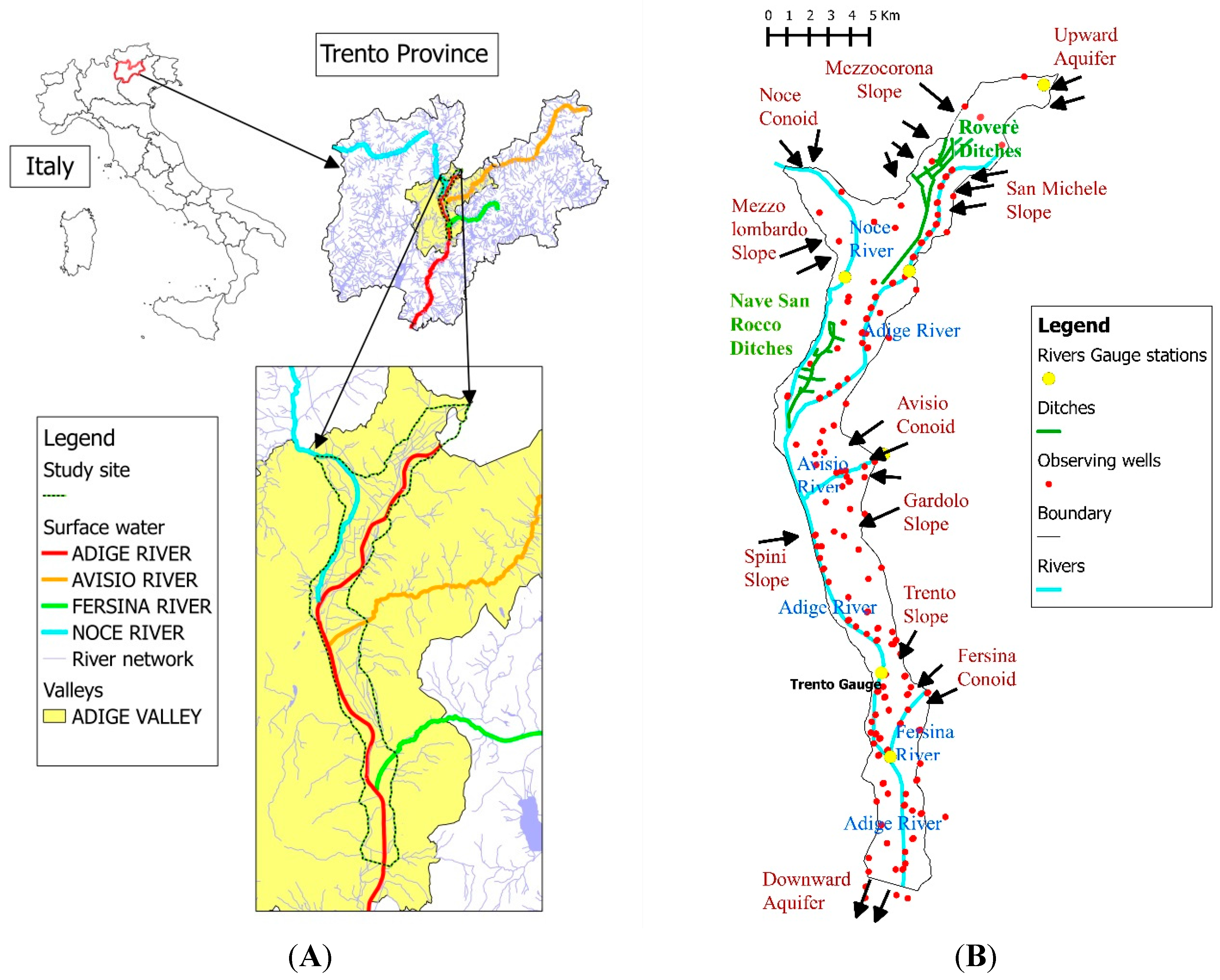
2.1. Site Description

The hydrology of the Adige catchment (9700 km² at Trento), is mainly controlled by snow and glacier melting (e.g., [47,48,49]), although it is also significantly influenced by anthropogenic activities such as hydropower production [50] and agriculture [48]. The catchment is characterized by a sub-alpine climate with a long-term mean annual precipitation of 1022 mm.

The area considered in the present study occupies the Adige Valley in proximity of the city of Trento (which is also included), North-Eastern Italy. The mean thickness of the unconfined aquifer is 40 m and extends over an area of 70 km² with a mean head gradient of 0.08%–0.09% (Figure 1A). Land use is distributed as follows: 47% rural zones, 33% forest and 20% urban areas.

Figure 1. (A) The Adige valley is highlighted in yellow, the aquifer considered in this study is delimited by a dashed black line, the red line indicates the Adige River and the three main tributaries, Noce, Avisio and Fersina, are indicated with the light blue, orange and green lines, respectively; (B) Conceptual model of the aquifer in the Adige Valley in proximity of Trento.

Figure 1. (A) The Adige valley is highlighted in yellow, the aquifer considered in this study is delimited by a dashed black line, the red line indicates the Adige River and the three main tributaries, Noce, Avisio and Fersina, are indicated with the light blue, orange and green lines, respectively; (B) Conceptual model of the aquifer in the Adige Valley in proximity of Trento.

The study area was originally a wetland, which was reclaimed in the late eighteenth century; since the reclamation, the entire area was highly exploited by agriculture with a significant freshwater request for irrigation (the mean annual flow is 1.83 m³/s [51]). Land reclamation was performed constructing a network of ditches, which drains the agricultural land and discharges the collected water into the Adige River and its main tributaries (i.e., Noce, Avisio and Fersina) in proximity of the confluences. When the water level in the rivers is higher than the ground level, dewatering pumps are activated to empty the ditches. The area considered in this study is interested by 23 dewatering systems, which can extract up to 68 m³/s. The presence of the ditches and their management are fundamental for agricultural activities and to regulate water uses. The ditches, in fact, are also used to distribute water used for irrigation during the dry periods. Only the two most spatially extended networks of ditches in the northern part of the area were considered in this study: Roverè della Luna and Nave San Rocco (Figure 1B).

The Adige River, the second in Italy for length, generated coarse alluvial fan deposits, which host the shallow aquifer considered in the present study. The river flows along the valley and its mean water discharge at the Trento gauging station is of 212 m³/s. Three important tributaries join the Adige River within the study area (Figure 1A). The Noce River has a mean water discharge of 46 m³/s and a timing strongly modified by four hydropower plants located within its catchment [50]. From entrance in the Adige valley, it flows for 11 km before joining the Adige River. The Avisio River has a mean water discharge of 23.5 m³/s, which is significantly smaller than the natural mean streamflow due to the diversion of water toward three hydropower systems with powerhouse outside the catchment. It flows for 3.2 km along the Adige valley before joining the Adige River. Finally, the Fersina River has a mean water discharge of 2.0 m³/s and flows in the Adige valley for 2.7 km before joining the Adige River.

The aquifer is recharged also by lateral springs mainly in correspondence to the alluvial fans of Avisio, Fersina and Noce (Figure 1B). The aquifer is intensively exploited by 2070 wells and the vast majority of them (almost 78%) are used for agriculture. Their pumping rates vary seasonally according to crop needs [43]. The shallow aquifer is exploited also by the water supply system of the city of Trento with five well fields. The most important is located in the Avisio alluvial fan and its mean extraction rate is 208 l/s. The aquifer responds quickly to the external stressors [52], thereby justifying the steady-state assumption to simulate the aquifer behavior used in this study.

The hydraulic head data used to calibrate and validate the model were collected in 2008, during two field campaigns. The first campaign was conducted from 23 to 25 June, the second from 13 to 15 October [53]. The piezometric heads were measured in 102 wells (shown by red dots in Figure 1B) within the area of interest. The piezometric heads remained almost constant during each of the two campaigns, with maximum oscillations of about 0.1 m. Daily precipitation data are available at six rain gauges uniformly distributed in the area considered and managed by the Unità Operativa Sistema Informativo Geografico, Centro Trasferimento Tecnologico, Edmund Mach Foundation. During the two field campaigns, no rainfall events occurred.

2.2. Assessment Criteria

In this study, we consider three criteria, which can be used to take informed decisions about the management of groundwater resources. The computation of the assessment criteria and their uncertainty requires the knowledge of the head distribution and of the water fluxes into the aquifer. Such information is typically provided by a physically based mathematical model, which exploits available data. The flow equation is solved by the finite volume scheme implemented into MODFLOW [54] with a three-dimensional grid; consequently the computational cell is identified by three indexes: i (row number, along y), j (column number, along x) and k (layer number, along z).

The first assessment criterion is the depth to water (DTW) ([7,55]) which can be computed as follows:

$$DT{W}_{i,j}=DT{M}_{i,j}-h_{i,j}$$

(1)

where DTM_i,j (Digital Terrain Model) is the elevation of the ground surface at the cell i,j of a horizontal grid sharing in the horizontal plane the same nodes of the computational grid and h_i,j is the aquifer water level at the same position. Shallow aquifers are often endangered by surface contamination, hence the DTW is an important index of their vulnerability. In addition, DTW is also indicative of the costs of exploiting the aquifer, since the pumping cost depends on the hydraulic head, which in an unconfined aquifer is equal to the water level.

The second criterion describes the spatial distribution of the local recharges/discharges fluxes, which can be obtained by applying the local mass balance applied to the vertical column i,j (identified here with the horizontal nodes of the cells composing the column):

$$Q_{i-1,j}+Q_{i+1,j}+Q_{i,j-1}+Q_{i,j+1}=-R_{i,j}$$

(2)

where Q_i,j is the flow exchanged [L³/T] across the four columns (a parallelepiped with a rectangular base and height equals to the aquifer thickness) surrounding the central column i,j, and R_i,j is the groundwater recharge/discharge index [56,57,58]. The subscripts (i − 1,j), (i + 1,j), (i,j − 1) and (i,j + 1) identify the columns located to the South North and West, East of the cell (i,j), respectively (Figure 2A). Imbalances between inflows and outflows in a vertical column can occur only if $R_{i,j}$ differs from zero. Lin and Anderson [57], Lin et al. [58] and Stoertz and Bradbury [59] proposed a methodology for estimating the recharge/discharge rates based on water balance, which can be applied in conjunction with parameters estimation. In this study $R_{i,j}$ is known (when it represents the water pumped from the extraction wells and the infiltration water rate from the unsaturated soil) and is estimated thorough the inversion of the hydraulic head data available when it represents the exchange flux with surface water and with the lateral external aquifers.

Recharge/discharge estimation has been utilized for assessing the sustainability of aquifer exploitation [60,61]. The recharge areas for the aquifer are identified by positive values of $R_{i,j}$ and should be considered sensitive areas to protect against surface contamination. The areas characterized by negative values of $R_{i,j}$ are indicative of discharge zones, i.e., areas where the aquifer is drained. By comparing how the recharge/discharge pattern can be modified under different exploitation activity for the aquifer is crucial for evaluating sustainability of groundwater extraction.

As stated by Neff et al. [62], “An estimate of natural recharge, by itself, however, should not be used to determine the amount of ground water that can be withdrawn on a sustained basis. The quantity of ground water available for use depends more upon how the changes in inflow and outflow that result from withdrawals affect the surrounding environment and the acceptable tradeoff between ground-water use and these changes.” Numerical simulations allow computing the changes in inflow and outflow due to variations in pumping rates and hence to assess the capability of the aquifer to sustain a given water demand. A third metric S, called sustainability, is hence defined to describe the water productivity of the aquifer given the actual distribution and operation of pumping wells. We define as $Q_{i,j}^{out}$ the total flux integrated in the z direction at position (i,j), which similarly to the previous criteria, identify the horizontal projection of the vertical column along which flux is integrated, computed by the numerical model of the aquifer. Sustainability $S_{i,j}$ at the position (i,j) can be defined as:

$$S_{i,j}\left(∆W\right)= Q_{i,j}^{out}\left(W+∆W\right)- Q_{i,j}^{out}\left(W\right)$$

(3)

where $Q_{i,j}^{out}\left(W\right)$ is the outflow from the water column i,j computed according to the actual water management policy and $Q_{i,j}^{out}\left(W+∆W\right)$ is the outflow computed for the scenario with a modified water extraction from the aquifer of ∆W. The index $S_{i,j}\left(∆W\right)$ quantifies the response of the vertical water column to the variation in water demand.

The index S can be particularly useful to define the sustainability of different portions of the aquifer subjected to exploitation strategies. Indeed, the aquifer will respond to the increased discharge flux ∆W by decreasing $Q_{i,j}^{out}$ at locations where the increase of recharge (i.e., vertical flux) is less than that required to balance the larger extraction. This leads to a heterogeneous pattern of $S_{i,j}\left(∆W\right)$ and if $S_{i,j}\left(∆W\right)$ is larger or equal than zero, the aquifer at i,j can be considered able to sustain the increased outlet fluxes to face ∆W; on the contrary, if $S_{i,j}\left(∆W\right)$ is negative, the aquifer at i,j will suffer from an excessive extraction. The computational scheme is illustrated in Figure 2B,C. Let us assume that in the actual water management (Figure 2B) water is extracted at a rate R, while the same amount of water in injected into the eastern cell. In this case, Q_out for the central cell is given by the sum of Q₂, Q₃ and Q₄. If the water extraction activity increases in the central cell (Figure 2C) while the recharge rate remains the same in the eastern cell, the flow is redistributed among the other cells according to their recharge capacity (from the neighbor cells). Let us assume that only the northern cell is able to increase its Q_out in order to provide more water to the center cell (Q₂' > Q₂) whereas the southern and the western cells are less productive (Q₄' < Q₄ and Q₃' < Q₃), we observe a decrease in the Q_out values for the central, southern and western cells. This leads to positive values of $S_{i,j}$ (green in Figure 2C) for the north cell and to negative values of $S_{i,j}$ for the southern, western and central cells (red in Figure 2C). Therefore, $S_{i,j}\left(∆W\right)$ compares the initial condition of the aquifer, i.e., considering the actual wells distribution and extraction rates, against a new water management strategy. It is desirable that areas with $S_{i,j}\left(∆W\right)>0$ occur away from zones vulnerable to contamination, because their increased $Q_{i,j}^{out}$ to the neighboring cells may intensify the transport of contaminants, whereas areas with $S_{i,j}\left(∆W\right)<0$ can be considered less productive and not suitable for further water exploitation.

Figure 2. (A) Flow scheme utilized for computing the recharge/discharge index; (B) example of flow scheme with a recharge R in the eastern cell and a discharge R in the center cell; (C) example of flow scheme with a recharge R in the eastern cell and a discharge 2R in the center cell under the hypothesis that only the northern cell is able to increase its Q_out flux for sustaining the increase in the discharge rate in the center cell.

Figure 2. (A) Flow scheme utilized for computing the recharge/discharge index; (B) example of flow scheme with a recharge R in the eastern cell and a discharge R in the center cell; (C) example of flow scheme with a recharge R in the eastern cell and a discharge 2R in the center cell under the hypothesis that only the northern cell is able to increase its Q_out flux for sustaining the increase in the discharge rate in the center cell.

2.3. Physical Model for the Aquifer

In order to compute the assessment criteria described in Section 2.2, groundwater flow in the shallow aquifer of the Adige Valley was simulated under stationary conditions by using MODFLOW-2005 [54]. The computational domain was discretized using 8 layers each 5 m thick and a horizontal squared grid with side equal to 80 m (82,590 active cells in total). The top layer resembles the actual surface topography of the study site. Two different steady-state models are implemented: the first case (CASE 1) uses the average piezometric head distribution recorded in three days (23–25 June 2008); the second case (CASE 2) uses the average piezometric head recorded on 13–15 October 2008.

Extraction fluxes from wells are obtained from the Water Management Office of the Trento Province and the recharge flux from the unsaturated soil is simulated by using the 0-D model of the unsaturated zone described in Section 2.3.3. Also, the exchange flux between rivers/ditches and the shallow aquifer is accurately modeled by imposing along the rivers/ditches’ courses a Cauchy boundary condition (Section 2.3.1 and Section 2.3.2) and the recharge from the lateral aquifers is reproduced with Neuman boundary conditions in correspondence of alluvial fans and springs. Facies distribution, conditional to the available stratigraphic information, from which depends the value of the hydraulic conductivity assigned to the computational cells is generated stochastically by a Markov chain approach as described in Section 2.3.4.

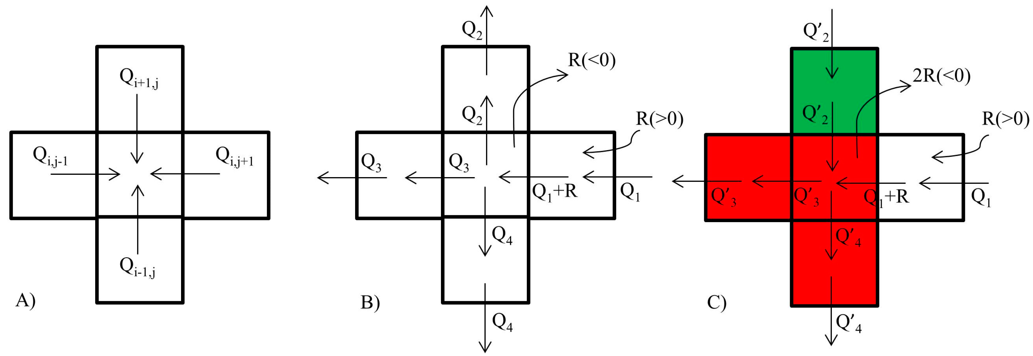
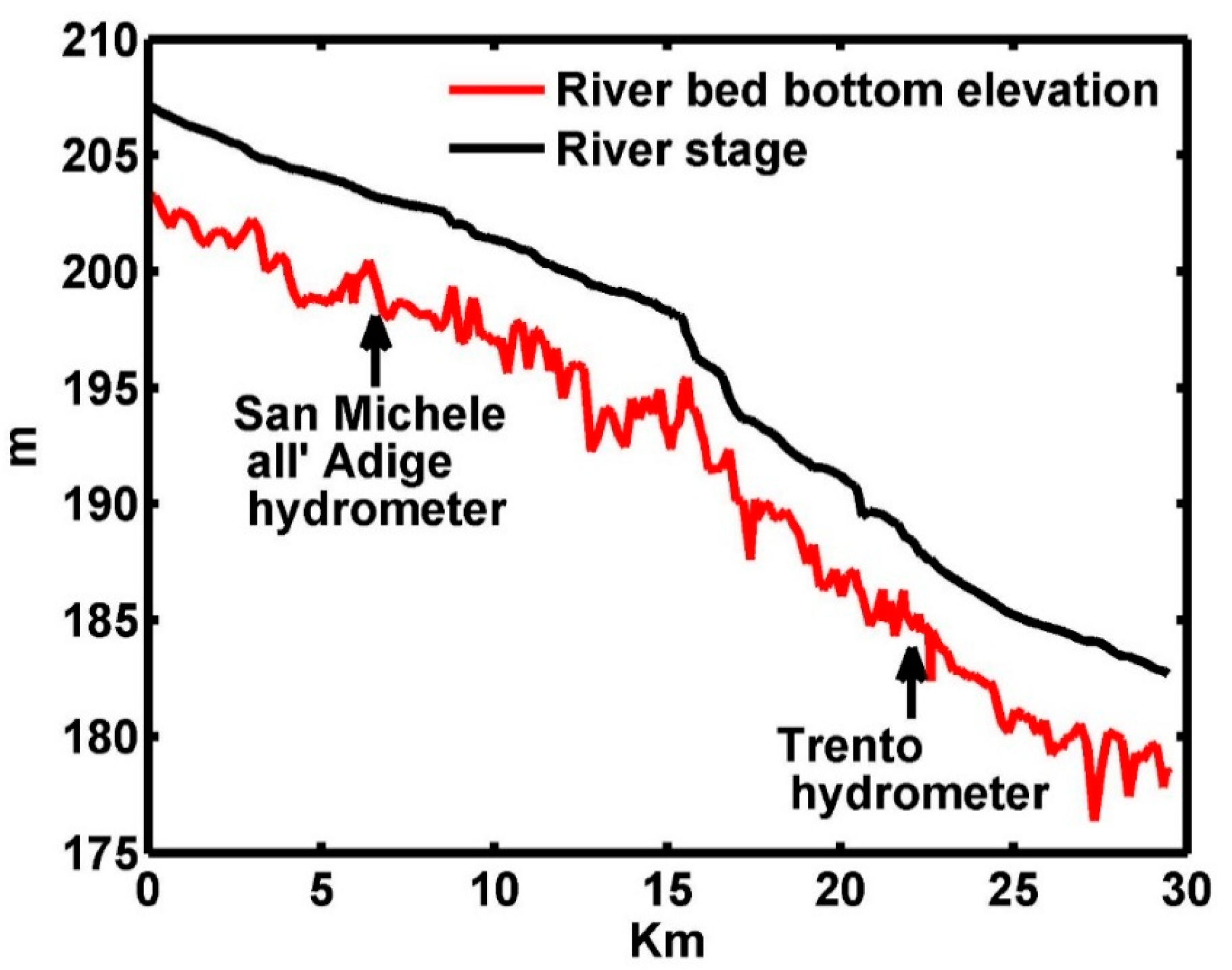
2.3.1. River–Aquifer Exchange Model

The rivers’ exchange flux with the shallow aquifer (Q_riv) was modeled using the river package implemented in MODFLOW-2005 [63]:

$$\begin{array}{c}{Q}_{\mathit{riv}}=C_{\mathit{riv}}(H_{\mathit{riv}}-h_{\mathit{ijk}}) \mathit{if} h_{\mathit{ijk}}>R_{\mathit{bot}}\\ Q_{\mathit{riv}}=C_{\mathit{riv}}(H_{\mathit{riv}}-R_{\mathit{bot}}) \mathit{if} h_{\mathit{ijk}}<R_{\mathit{bot}}\end{array}$$

(4)

where C_riv is the hydraulic conductance of the riverbed, H_riv is the hydraulic stage of the river and R_bot is the river bed elevation. Reproducing the effects of the surface water/groundwater exchange on aquifers dynamics is challenging because the hydraulic conductance C_riv is hardly identifiable from piezometric head measurements, while they are crucial to the evaluation of the exchange fluxes [64] and depend also on the computational grid size [65]. Furthermore, Lackey et al. [66] showed that the hydraulic conductance of the riverbed is spatially variable. In the present study, we adopt a block type heterogeneous distribution of the hydraulic conductance of the riverbed. To this purpose, the Adige course was split into four segments (0 to 3 km/3 to 13 km/13 to 26 km/26 to 30 km) characterized by four different values of C_riv, while a single value of C_riv was considered sufficient to characterize each of the tributaries. The Adige riverbed bottom elevation (Figure 3) was obtained by the longitudinal profile of the river with a discretization of 200 m, updated in 1996 [65]; the riverbed of the Noce, Avisio and Fersina Rivers have been extrapolated from the DTM of the Trento Province (Lidar 2007, Provincia Autonoma di Trento). The River stage along the course of the Adige River (Figure 3) was computed by solving the one dimensional shallow water equation with a numerical model implemented in the flood protection and warning system of the Adige River in use at the Office of Risk Prevention of the Trento Province, by using a grid spacing of 200 m.

Figure 3. Riverbed bottom elevation for the Adige River and the river stage computed with variable water discharge along the course equal to the mean recorded during the period 23 to 25 June 2008.

Figure 3. Riverbed bottom elevation for the Adige River and the river stage computed with variable water discharge along the course equal to the mean recorded during the period 23 to 25 June 2008.

The simulations were performed using the average flow recorded at San Michele all’Adige and Trento Ponte San Lorenzo gauging stations (Figure 1B), which in the CASE 1 (23–25 June 2008) amount to 303 m³/s and 425 m³/s, respectively. In CASE 2 (13 to 15 October 2008) the flow rates are reduced to 100 m³/s and 147 m³/s, respectively. For the Noce, Avisio and Fersina Rivers, the river flows were considered constant along their course and the river stages were computed with the Chezy formulation for uniform flow [67], using the roughness coefficient computed at the gauge station by using the rating curve.

2.3.2. Ditches–Aquifer Exchange Model

The ditches interact with the aquifer in two ways, depending on their functioning. In this study, we model two possible interactions between groundwater and the ditches. In a first case, the ditches are represented as drains. In a second case, the water level inside the ditches is kept constant to reproduce operations conducted during irrigation periods through the combined use of gates and inflow from the Noce River.

In the first case, the exchange flux was simulated through the drain package of MODFLOW-2005 [63] which computes the flux from the aquifer to the ditches by using Equation (4) but considering H_riv = R_bot. The ditches bottom elevation was obtained from the 2 m resolution DTM of the Province of Trento. In the second case, the ditches are simulated through the river package of MODFLOW-2005 [63] which computes the flux from the ditches to the aquifer by using Equation (4) under the assumption that the water stage is constant in all the ditches forming the network and equal to 0.5 m (H_riv − R_bot = 0.5 m) [68]. The riverbed conductance was considered constant for the two networks of ditches

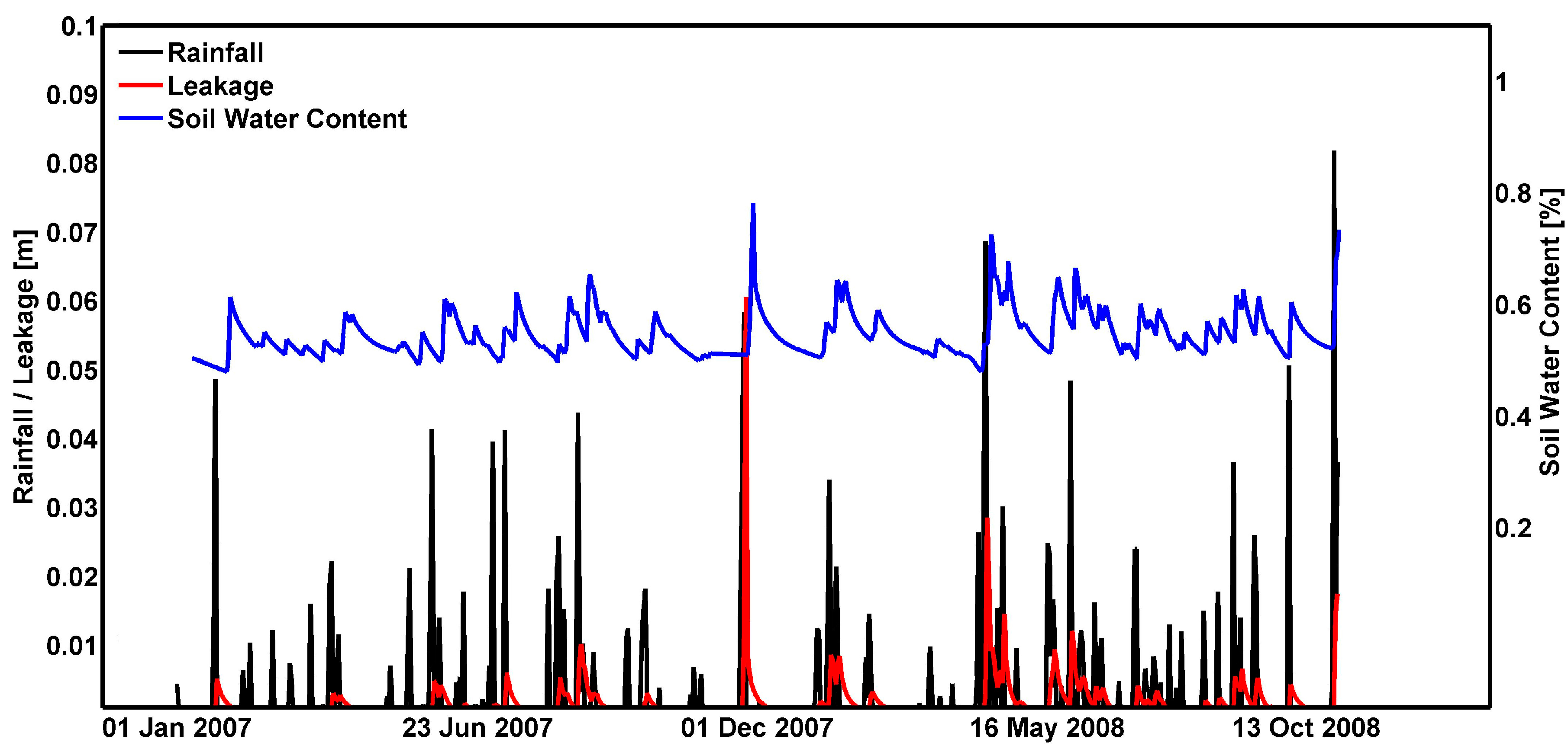
2.3.3. Leakage Model

The recharge of the aquifer was simulated by using the recharge package of MODFLOW [63], which requires that the infiltration is assigned to each computational cell of the first layer. In urban areas, the infiltration has been set to zero, while in the rest of the domain the infiltration has been computed by averaging the leakage L over the periods 23 to 25 June 2008 (CASE 1) and 13 to 15 October 2008 (CASE 2). The leakage depends on soil water dynamics in the unsaturated zone above the aquifer and was modeled using the following balance equation [69]:

$$n{Z}_r\frac{d\mathrm{\text{θ}}\left(t\right)}{dt}=P\left(t\right)+Irr\left(t\right)-ET\left[\mathrm{\text{θ}}\left(t\right),t\right]-L\left[\mathrm{\text{θ}}\left(t\right)\right]$$

(5)

where n is the soil porosity, Z_r is soil thickness of the unsaturated zone, θ∈(0,1) is the degree of saturation, P is the rainfall, Irr is the irrigation flux and ET is the evapotranspiration. It is assumed that runoff takes place when the rainfall overcomes the available storage into the soil. The degree of saturation θ(t) is computed explicitly with a time step of one day from the 1 January 2007 to 25 October 2008:

$$\begin{array}{c}\mathrm{\text{θ}}\left(t\right)=\frac{P\left(t\right)+Irr\left(t\right)-ET\left[\mathrm{\text{θ}}\left(t-1\right)\right]-L\left[\mathrm{\text{θ}}\left(t-1\right)\right]}{n{Z}_r}∆t \end{array}$$

(6)

The Rainfall P(t) was obtained by spatial interpolation of daily precipitations recorded at the six closest meteorological stations (Gardolo, Mezzolombardo, Roverè della Luna, San Michele all’Adige, Trento sud, Zambana). The daily irrigation rate was obtained by the monthly averaged measurements available from [70] under the simplifying assumption of a constant daily rate through the month. If the resulting θ(t) is larger than 1, the excess of water Q₀(t) = [θ(t)−1] × n × Z_r is available for runoff and θ(t) is set to 1, before moving to the next step. The external forcing P(t) and Irr(t) were assigned to each cell by interpolation with the Thiessen polygons. Finally, ET was represented through the following model [71]:

$$ET\left(\mathrm{\text{θ}}\right)=\{\begin{array}{c}\frac{\mathrm{\text{θ}}-{\mathrm{\text{θ}}}_h}{{\mathrm{\text{θ}}}_w-{\mathrm{\text{θ}}}_h}{E}_w if {\mathrm{\text{θ}}}_h<\theta \le {\mathrm{\text{θ}}}_w\\ E_w+\left(E_{max}-E_w\right)\frac{\mathrm{\text{θ}}-{\mathrm{\text{θ}}}_w}{{\mathrm{\text{θ}}}^{*}-{\mathrm{\text{θ}}}_w} if {\mathrm{\text{θ}}}_w<\theta \le {\mathrm{\text{θ}}}^{*} \\ E_{max} if {\mathrm{\text{θ}}}^{*}<\theta \le 1\end{array}$$

(7)

where E_max is the potential evapotranspiration, which depends only on meteorological variables and is independent from θ, θ_w is the wilting point and E_w is the correspondent evapotranspiration loss, θ* represents the soil moisture content below which the plant starts to reduce transpiration to protect stomata and θ_h is the hygroscopic point. In the present study, we used for E_max, which depends on the cultivated crop and the type of spontaneous vegetation, the estimates proposed by [70].

The leakage was hence computed as [71]:

$$L\left(\mathrm{\text{θ}}\right)=\frac{K_s}{e^{\text{β}\left(1-{\mathrm{\text{θ}}}_{fc}\right)}-1}\left[e^{\text{β}\left(\mathrm{\text{θ}}-{\mathrm{\text{θ}}}_{fc}\right)}-1\right] if {\mathrm{\text{θ}}}_{fc}<\mathrm{\text{θ}}\le 1$$

(8)

where K_s is the saturated hydraulic conductivity, θ_fc is the saturation at the field capacity, and β = 2b + 4 where b is an empirical parameter used in the soil-water retention curve: Ψ_s = Ψ*_s θ^−b, where Ψ_s is the water potential and Ψ*_s is another empirical parameter, which depends on the type of soil. It varies from 12 for sand to 26 for clay. The characteristic soil in the Adige Valley can be categorized as loamy sand, therefore the parameters utilized are listed in Table 1, reproduced from Laio et al. [69]. Figure 4 shows as illustrative example the recharge L simulated in a cell located in the northern part of the study area (x_utm = 667,798; y_utm = 5,124,101).

Table 1. Parameters of the leakage model (reproduced from Table 1, Section 2.6 of [68]).

$\beta$	$K_s(\frac{m}{d})$	$E_w(\frac{m}{d})$	$s_{fc}$	$s_h$	$s_w$	$s^{*}$	$n$	$Z_r(m)$
12.7	1.0	0.0001	0.52	0.08	0.11	0.31	0.42	1.0

Table 1. Parameters of the leakage model (reproduced from Table 1, Section 2.6 of [68]).

$\beta$	$K_s(\frac{m}{d})$	$E_w(\frac{m}{d})$	$s_{fc}$	$s_h$	$s_w$	$s^{*}$	$n$	$Z_r(m)$
12.7	1.0	0.0001	0.52	0.08	0.11	0.31	0.42	1.0

Figure 4. Simulated time series of soil water content (blue line) and leakage (red line) at the position (x_utm = 667,798; y_utm = 5,124,101) of the Adige valley. Precipitation is also shown (black bars).

Figure 4. Simulated time series of soil water content (blue line) and leakage (red line) at the position (x_utm = 667,798; y_utm = 5,124,101) of the Adige valley. Precipitation is also shown (black bars).

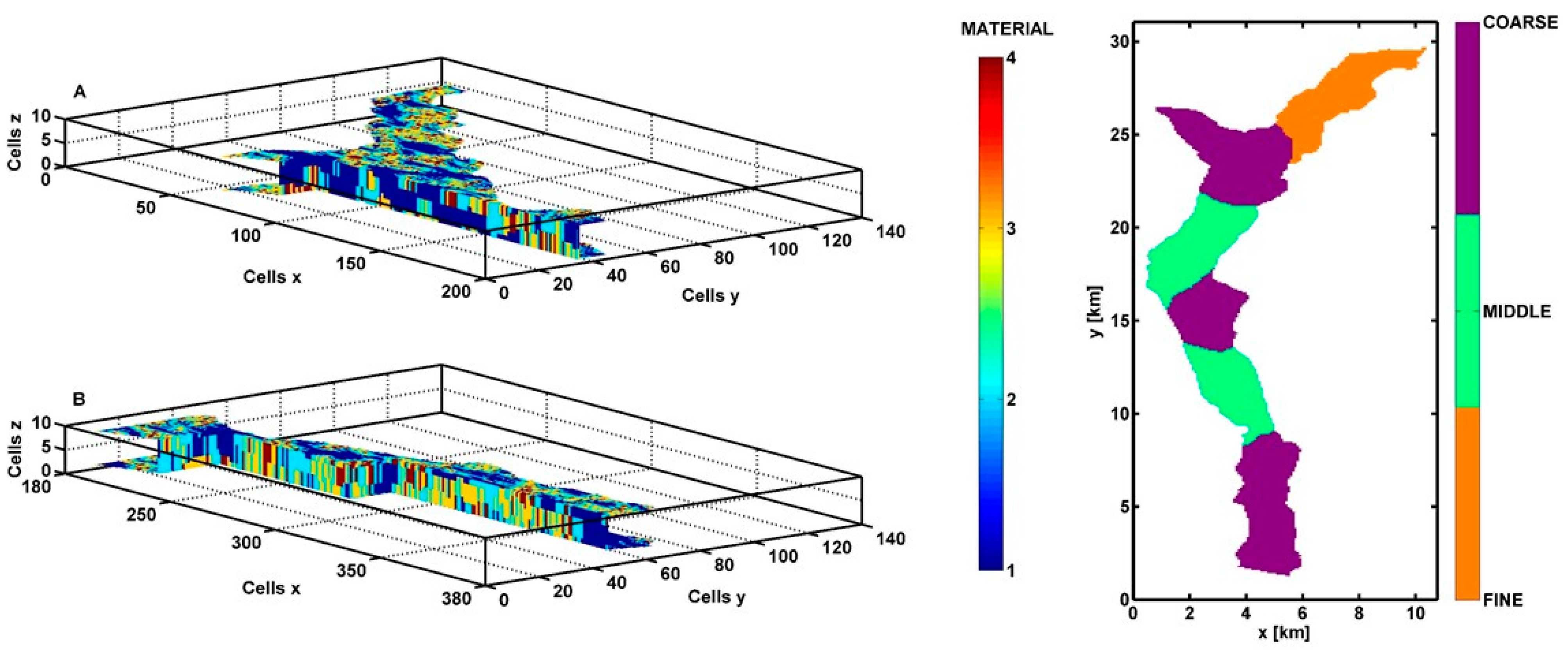
2.3.4. Heterogeneous Hydraulic Conductivity Fields

The shallow aquifer of the Adige Valley is heterogeneous, as evidenced by the 1068 stratigraphic boreholes of the area. Initially, the soil types extracted from the available stratigraphy at the boreholes have been grouped in four material classes identified according to the soil texture and ordered by decreasing values of hydraulic conductivity as Material 1, 2, 3 and 4. Heterogeneous hydraulic properties have been generated stochastically by using T-PROGS [44], a Markov chain transition probability method [72]. T-PROGS generates random realizations of hydrofacies conditional to borehole information by using a suitable sequential indicator simulation scheme [72] with the cross indicator semivariograms between two points at reciprocal distance d given by the following transition probability:

$$t_{m1,m2}\left(d\right)=\text{Pr}\{m_2 at x+d|m_1 at x\}$$

(9)

which quantifies the probability of observing the material m₂ at x + d provided that the material m₁ has been observed at x. Since the inspection of stratigraphy identified four materials, the transition probabilities assume the form of a 4 × 4 matrix T(d_φ):

$$T\left(d_{\text{φ}}\right)=\text{exp}\left(R_{\text{φ}}{d}_{\text{φ}}\right)$$

(10)

where R_φ is the transition rate matrix:

$$R_{\text{φ}}=\left(\begin{array}{ccc}{r}_{m1m1,\text{φ}}& \cdots & r_{m1m4,\text{φ}}\\ ⋮& \ddots & ⋮\\ r_{m4m1,\text{φ}}& \cdots & r_{m4m4,\text{φ}}\end{array}\right)$$

(11)

In Equations (9) and (10), φ indicates the three components (d_x, d_y, d_z) of the two-point separation distance. The diagonal terms of R_φ are related to the mean length (L) of the facies along the direction φ:

$$r_{mlml,\text{φ}}=-\frac{1}{L_{l,\text{φ}}} , l=1,\dots .,4$$

(12)

which is determined by means of prior geological interpretations of the hydrofacies configuration. The mean facies lengths along the three coordinate directions are shown in Table 2.

Table 2. Proportions of materials and the corresponding mean lengths utilized for the T-PROGS simulations.

		Mean Length (m)
Material	Volume Fraction (%)	X (strike)	Y (dip)	Z (vertical)
1	30.0	100.0	510.0	6.02
2	39.0	41.3	55.0	3.4
3	20.0	63.2	63.0	3.11
4	11.0	58.0	58.0	3.87

Table 2. Proportions of materials and the corresponding mean lengths utilized for the T-PROGS simulations.

		Mean Length (m)
Material	Volume Fraction (%)	X (strike)	Y (dip)	Z (vertical)
1	30.0	100.0	510.0	6.02
2	39.0	41.3	55.0	3.4
3	20.0	63.2	63.0	3.11
4	11.0	58.0	58.0	3.87

Two views of one of the 25 T-PROGS simulations we used in the present work are shown in Figure 5A,B.

Figure 5. Example of the generated hydraulic conductivity fields (A to B); zonation for the hydraulic conductivity values (C).

Figure 5. Example of the generated hydraulic conductivity fields (A to B); zonation for the hydraulic conductivity values (C).

The computational domain is divided in three homogeneous zones (see the zones with the same color in Figure 5C named COARSE (C), MIDDLE (M) and FINE (F). In each zone, a constant hydraulic conductivity is assigned to the material and this value may change through the zones according to the indications emerging from the available geological interpretation and field tests [43]. Therefore, 12 parameters, i.e., the hydraulic conductivity of the four materials in the three zones, suffice to describe the spatial variability of the hydraulic properties.

2.4. Parameter Estimation and Uncertainty of the Assessment Criteria

Let us define V as the vector containing the values that each assessment criterion assume at the selected cells within the area of interest (the assessment criteria are evaluated at the horizontal cells of the computational grid, for example at the surface cells of the first layer), and Z the vector of the available head measurements. Since the main source of uncertainty is the spatial distribution of the hydraulic conductivity, the uncertainty of V will be computed in a Monte Carlo framework, by generating a number of independent realizations of hydrofacies, by using T-Progs as described in Section 2.3.4.

For each Monte Carlo realization, the N_a = 31 unknown parameters A (listed in the Supplementary Material in Tables S1–S3) were calibrated for CASE 1 by minimizing the absolute difference between the measured and simulated heads at 102 observation points (piezometers or wells). In the CASE 2, referring to the piezometric heads measured in October 2008, the parameters were kept fixed to the values obtained in the CASE 1 with exception of the 11 lateral flows, which show seasonal variability and hence were calibrated anew by using the new head measurements. In doing that, CASE 2 constitutes the validation of the 20 structural parameters ideally independent from the hydrodynamic conditions of the aquifer as dictated by the boundary conditions. They are 12 hydraulic conductivities and eight river conductances.

In each Monte Carlo realization, the combination of parameters that minimizes the following objective (fitness) function:

$$L={\displaystyle \sum }_{i=1}^{Nobs}|Z_i-{Z^{*}}_i|$$

(13)

is identified by using the particle Swarm Optimization (PSO) algorithm [73]. In Equation (13), Nobs is the number of observing wells, Z are the head measurements available and Z* are the simulated heads at the observation wells. The PSO algorithm allows exploring the space of the parameters to identify the combination of parameters that minimizes the objective fitness function (13).

In CASE 1, the space dimensionality is Na = 31, while in CASE 2, Na = 11 and according to the results of previous studies [74,75], the search was performed with the PSO by using N_p = 15 particles and N_s = 220 iterations, for a maximum of 3300 forward runs for each Monte Carlo realization.

The forward problem to be solved is strongly non-linear, such that certain combinations of the parameters A may led to a non-converging flow solution. During inversion, PSO may encounter a non-convergent solution and this circumstance has been dealt with by modifying the process in order to not consider solutions with the absolute value of the flow budget imbalance larger than 0.0001%.

The number of Monte Carlo realizations is chosen to ensure convergences of the statistics (first and second moments) of the vector V. In the present study, convergence was achieved with 25 Monte Carlo realizations. This relatively small number of realizations is the result of the information introduced by the head measurements in combination with the optimization step, which limits the variability across the realizations, since realizations not complying with the observational data (the vector Z) are ruled out by the PSO algorithm. Consequently, the sample frequency, computed by using the 25 realizations of the vector V containing the values of the selected assessment criterion at the grid cells can be computed as follows:

$$f_{V|Z}\left(V_i\right)\cong \frac{n_i}{MC \text{Δ}{V}_i}$$

(14)

where n_i is the number of elements in the sample contained within the interval $\text{Δ}{V}_i$ centered at V_i and MC is the sample dimension (i.e., the number MC of Monte Carlo realizations). The Equation (14) approximates the a-posteriori probability density function (PDF) $f_{V|Z}\left(V\right)$, which characterizes the uncertainty of the assessment criterion.

The associated Cumulated Distribution Function (CDF), which provides the probability of not exceeding a given value $\overline{Vi}$, can be estimated under the hypothesis that the Na parameters are independent:

$$P_{V|Z}\left(Vi<\overline{Vi}\text{|}Z\right)= \underset{-\infty }{\overset{\overline{V}}{{\displaystyle \int }}}{f}_{V|Z}\left(V_i\right) dV\cong {\displaystyle \sum }_{i=1}^n{f}_{V|Z}\left(V_i\right)\text{Δ}{V}_i$$

(15)

where n identifies the interval $\text{Δ}V$ in the discretization of the sample containing $\overline{V}$. This procedure corresponds to the Maximum a Posteriori (MAP) methodology applied to each Monte Carlo realization, already used with success in the inference of model parameters in subsurface hydrology (see e.g., [23,74,76]) and differs from GLUE (generalized likelihood uncertainty estimation) [77] because it does not require the introduction of a rejection criterion for non-behavioral models. Notice that the uncertainty analysis for V is applied under the assumption that uncertainty is chiefly controlled by the spatial distribution of the hydro-geological facies. The only valuable alternative to MAP in our view is to perform the inversion by fully exploring the space of the parameters as suggested in [78], with a dramatic increase of the computational burden. Exploring the interplay between uncertainty in facies geometry and model parameters is beyond the scope of the present contribution.

3. Results and Discussion

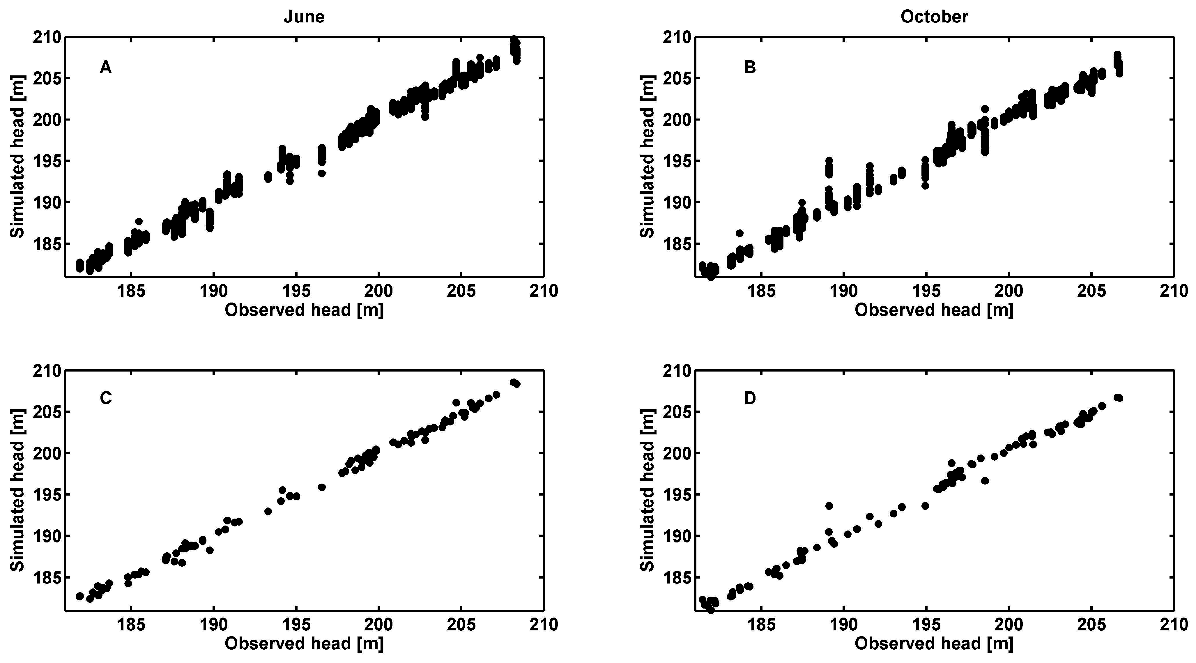
3.1. Calibration and Validation of the Numerical Model

Figure 6A shows the measured heads at the observation points in June 2008 versus the simulated vales for the 25 Monte Carlo simulations of the CASE 1. In this case, 31 unknown parameters have been calibrated (12 hydraulic conductivities plus 11 lateral flows, and eight river/ditches conductances). Similarly, Figure 6B repeats Figure 6A, considering instead the measuring campaign of October 2008 (CASE 2) and calibrating only the 11 external fluxes, while the remaining 20 parameters are the same as those obtained in the CASE 1.

Figure 6C,D show simulated versus observed heads in the best realization for the CASE 1 and 2, respectively. The root mean squared errors (RMSE) between observed and simulated heads ranges, among the 25 Monte Carlo simulations, from a minimum of 0.49 m to a maximum of 0.67 m for the CASE 1 and from 0.7 to 0.9 m, for the CASE 2. The result shows a good agreement between the simulations and the observations, with a slight increase of the error in the CASE 2. The validation process, however, highlights how the model parametrization utilized is suitable for reproducing the aquifer behavior. The sensitivity of the model to the calibration parameters is briefly discussed in the Supporting Information.

Figure 6. Simulated versus observed hydraulic heads for the CASE 1 and CASE 2 considering all Monte Carlo realizations ((A) and (B), respectively) and considering only the realization with the best fitness (i.e., the smallest L (Equation (13))) ((C) and (D), respectively).

Figure 6. Simulated versus observed hydraulic heads for the CASE 1 and CASE 2 considering all Monte Carlo realizations ((A) and (B), respectively) and considering only the realization with the best fitness (i.e., the smallest L (Equation (13))) ((C) and (D), respectively).

3.2. Assessment Criteria Evaluation

The comparison between the base case describing the actual situation and four water management scenarios reported in Table 3 is evaluated with reference to the three assessment criteria described in Section 2.2. Scenario RS05 shows the effects on the aquifer of varying streamflow and thereby river stages. This case is relevant because informative about the impact of a possible change in the management policies for hydropower production (e.g., a reduction of the ecological flow downstream hydropower water diversions). Scenarios PW2, PW5A and PW5B have been introduced to evaluate the effect of increasing water extraction from wells, in combination with the management of the ditches, for agricultural use. In particular, in Scenarios PW2 and PW5A, the ditches can only drain water from the aquifer, whereas in Scenario PW5B the ditches are refilled with surface water and their water level is kept constant. The objective of these simulations is to quantify how the uncertainty affecting hydraulic properties and socio-economic constraints, such as the actions related to management decisions, propagate into the uncertainty of the assessment criteria. For the sake of clarity, we analyze each criterion in a separate section. For practical purposes, however, all three assessment criteria should be considered and integrated in order to better identify novel water management strategies.

Table 3. Summary of the main features of the investigated scenarios.

Name	Description
Base	CASE 1 (Calibrated shallow aquifer model for June 2008)
RS05	CASE 1 with the rivers stage halved
PW2	CASE 1 with the rate of each pumping well doubled and assuming that the ditches quickly drain the water from the aquifer
PW5A	CASE 1 with the rate of each pumping well quintupled and assuming that the ditches quickly drain the water from the aquifer
PW5B	CASE 1 with the rate of each pumping well quintupled and assuming that the ditches are able to store water and are refilled by surface water.

Table 3. Summary of the main features of the investigated scenarios.

Name	Description
Base	CASE 1 (Calibrated shallow aquifer model for June 2008)
RS05	CASE 1 with the rivers stage halved
PW2	CASE 1 with the rate of each pumping well doubled and assuming that the ditches quickly drain the water from the aquifer
PW5A	CASE 1 with the rate of each pumping well quintupled and assuming that the ditches quickly drain the water from the aquifer
PW5B	CASE 1 with the rate of each pumping well quintupled and assuming that the ditches are able to store water and are refilled by surface water.

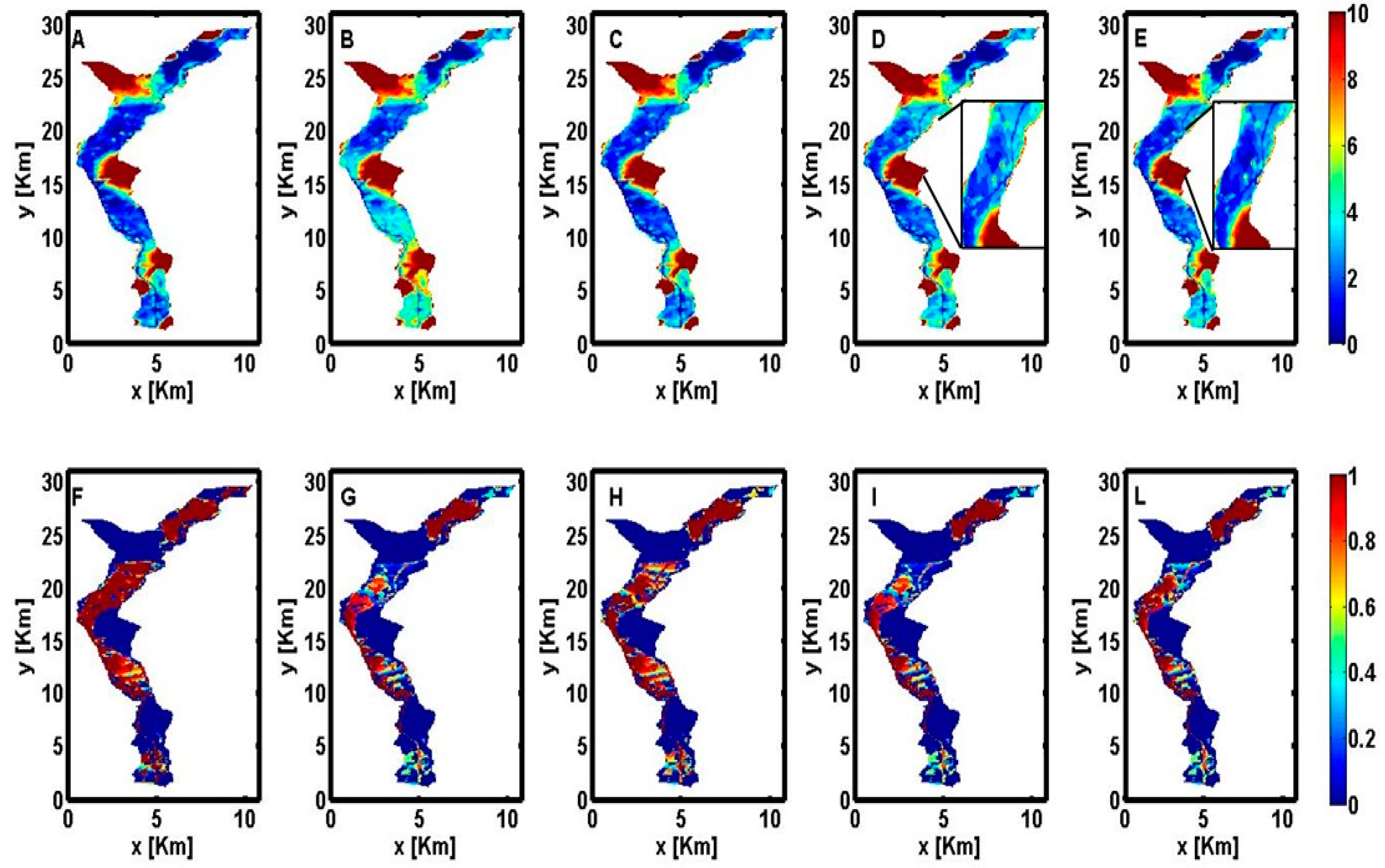
3.2.1. Depth to Water

The mean DTW computed in all 25 Monte Carlo simulations for the base case and for the four different scenarios, are shown in Figure 7A–E, respectively. For June 2008 (Figure 7A), the DTW does not exceed 5 m, except for the main alluvial fans and slopes, showing that the shallow aquifer is potentially vulnerable to superficial sources of contaminations. The model results show that in the northern part of the domain, some DTW values are negative. This may be explained with the presence of low conductive superficial hydrogeological unit confining the aquifer from above. The presence in this zone of a surficial loamy clay layer 10 to 15 m thick, as evidenced by Beretta [43], can provide a plausible explanation of this behavior, though it cannot source independent confirmation from observational data because of the very low density of observation wells in this area (Figure 1B). However, the rather shallow water table in the valley is indicative of a general vulnerability of the aquifer to contamination.

At the confluence of Noce and Avisio Rivers with the Adige River, the results of the model indicate a phreatic level close to the topographic surface, as also confirmed by the presence of natural wetlands, rich in flora and fauna. Figure 7B shows that halving the river stage leads to an increase of the water depth in the valley (i.e., reduction of the water level). Pumping activities should therefore be regulated also according to the Adige River stage, in order to preserve the wetlands. As expected, an increase of the pumping rate leads to a larger DTW as can be observed by comparing Figure 7C,D. In scenario PW2 (Figure 7C) and PW5A (Figure 7D), the pumping rate is two times and five times larger, respectively, than the pumping rate of Figure 7A. The largest increase of DTW is observed in the area where the Noce alluvial fan penetrates into the Adige Valley and in the southern portion of the domain. This can be explained considering the high density of wells present in these area. Figure 6E shows the effects of the recharge from the Nave San Rocco ditches on DTWs of the corresponding area (compare the inset of Figure 7D,E). A continuous refill of the ditches (scenario PW5B) leads to a slightly lower DTW values than in scenario PW5A. The DTW values in the northern part of the domain, however, are not significantly affected by both the river stage and the pumping rate, as can be observed by comparing Figure 7C–E with Figure 7A,B.

It is important for management and risk assessment analyses to define a critical threshold for the DTW. In the Adige aquifer, the wells utilized for irrigation have a depth varying between 5 and 10 m and the DTW should not exceed 2 m to guarantee their regular functioning. We compute therefore the probability of not exceeding this threshold within the domain, by using the results of the Monte Carlo simulations (Figure 7F–L).

Figure 7. Maps of the mean DTWs for the base case (A); and scenarios RS05, PW2, PW5A and PW5B (panels (B) to (E) in the first row). In addition, probability of DTW not exceeding the threshold of 2 m is shown for the base case (F) and the four scenarios RS05, PW2, PW5A, PW5B (panels (G) to (L) in the second row).

Figure 7. Maps of the mean DTWs for the base case (A); and scenarios RS05, PW2, PW5A and PW5B (panels (B) to (E) in the first row). In addition, probability of DTW not exceeding the threshold of 2 m is shown for the base case (F) and the four scenarios RS05, PW2, PW5A, PW5B (panels (G) to (L) in the second row).

Figure 7F shows that in the base scenario uncertainty affecting the DTW is relatively small, with an averaged (on all the Monte Carlo simulations) coefficient of variation of 8.8 × 10⁻². This result depends on the fact that the simulations considered here are obtained with the parameters that minimize the deviation between observed and simulated hydraulic heads. By increasing the extraction rate (Figure 7H,I,L), the zones with a lower probability of a DTW smaller than 2 m, are more extended than in Figure 7A. However, uncertainty in this case does not impact the general interpretation of the result, since most of the domain is characterized by a probability to exceed the given threshold either close to zero (blue) or one (red). This assessment criterion is therefore robust and it is not particularly prone to large variations caused by uncertainty in the distribution of hydro-geological facies.

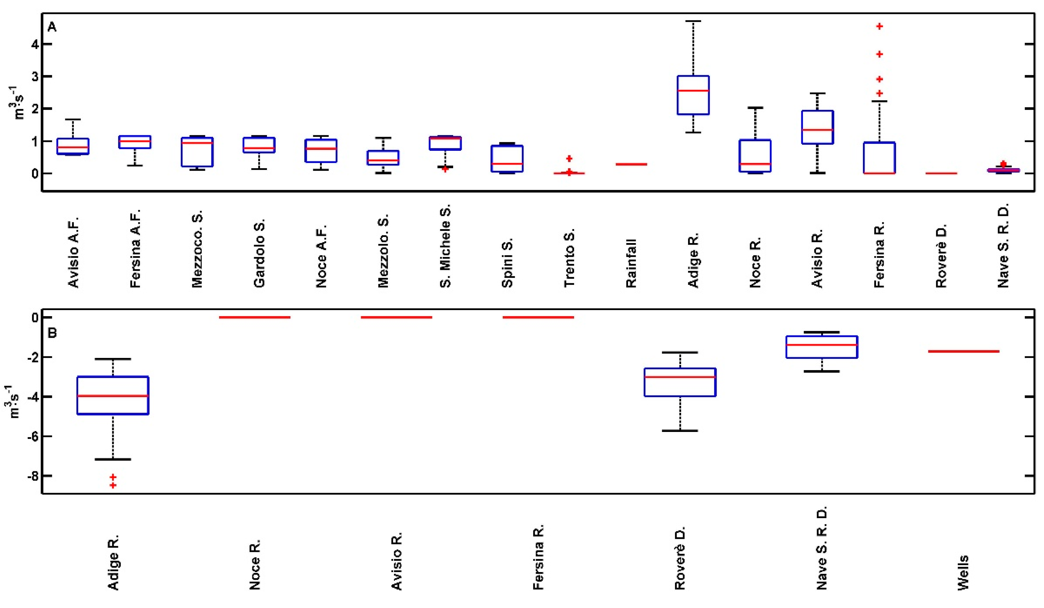
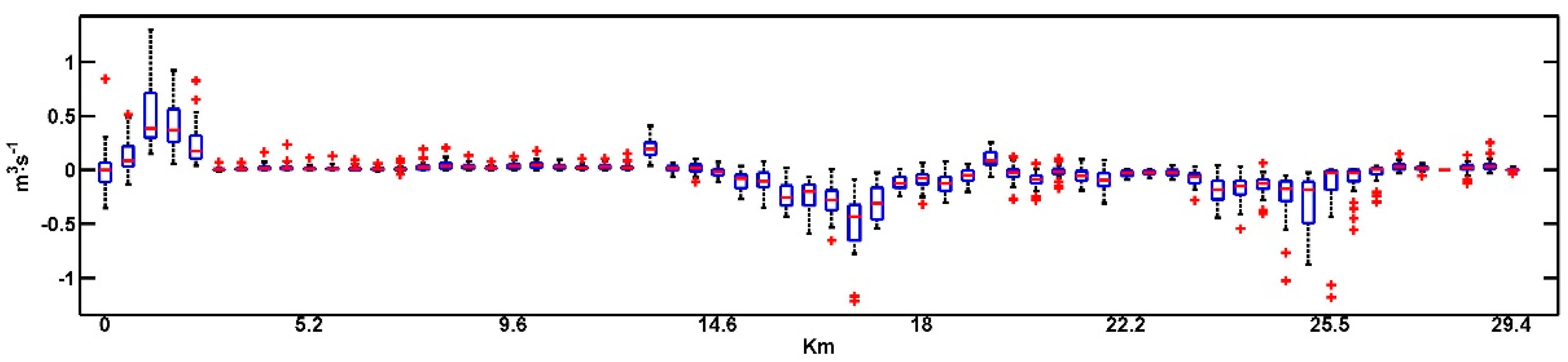
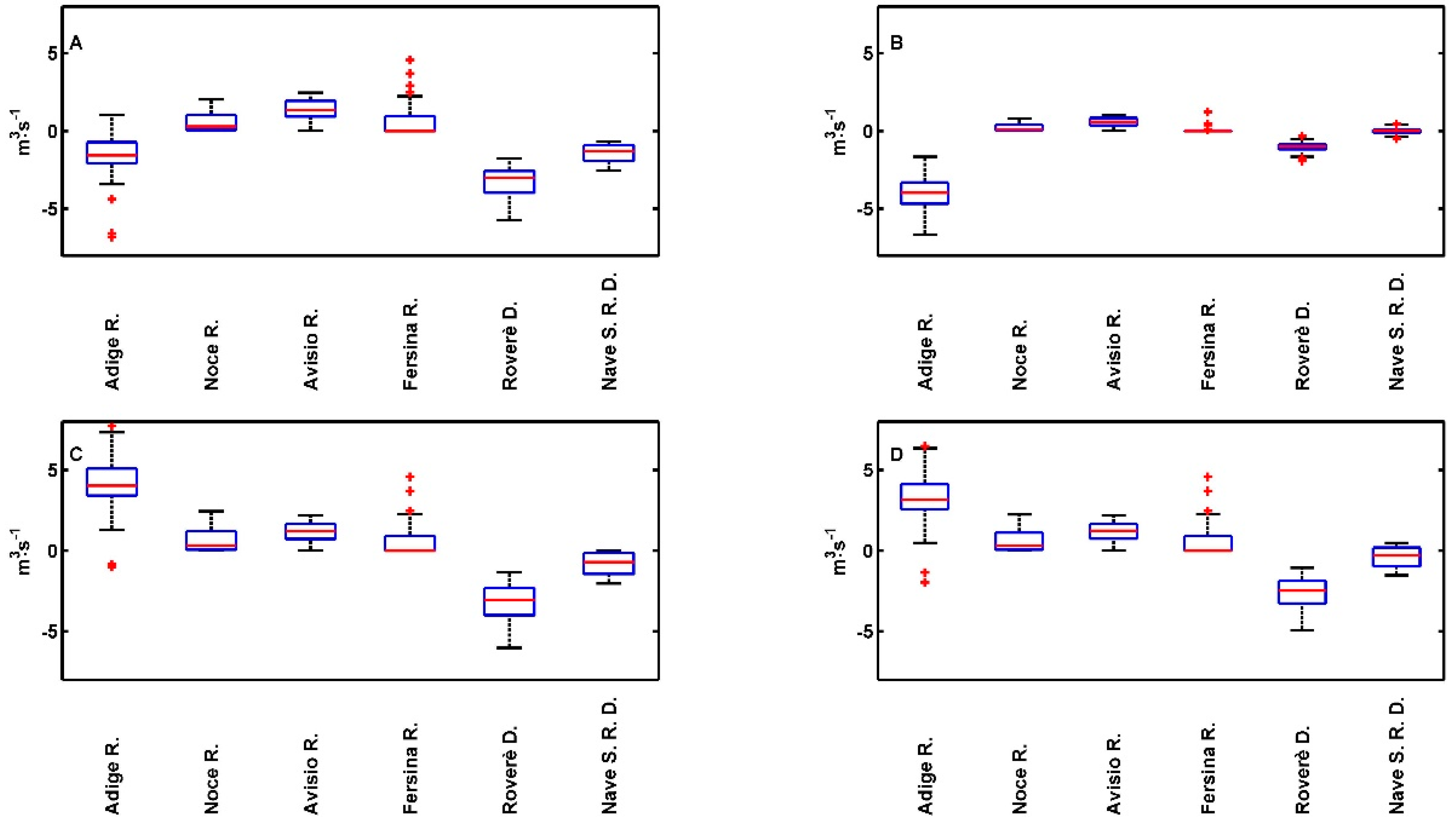
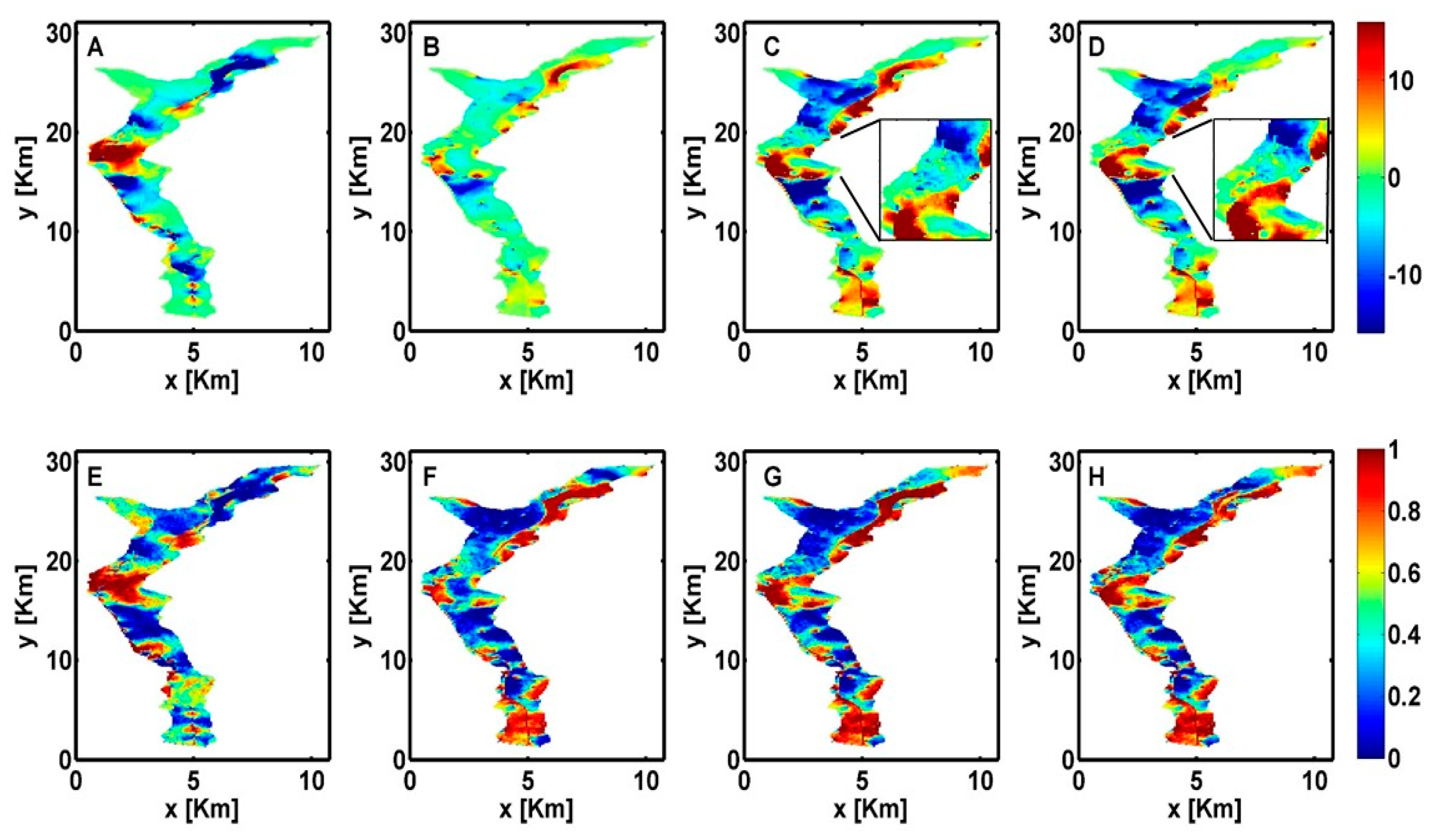
3.2.2. Recharge/Discharge Analysis

For the sake of illustration, we show the values of the recharge/discharge criterion grouped for the same type of source and sink. This index is therefore computed as the sum of the R_i,j of all the cells interacting with the same source/sink (i.e., the Adige River, the Avisio River, the Noce River, the Fersina River, the Roverè Ditches, the Nave San Rocco Ditches and the lateral exchange flows highlighted in red in Figure 1B). Figure 8A,B show the boxplots of the positive and negative exchange fluxes of the aquifer with the surface water and the lateral aquifers, respectively, computed with reference to the 25 Monte Carlo simulations of CASE 1.

Figure 8. (A) Boxplots of the recharge of the aquifer; (B) Boxplots of the discharge from of the aquifer.

Figure 8. (A) Boxplots of the recharge of the aquifer; (B) Boxplots of the discharge from of the aquifer.

The Adige River is the main source/sink of water for the shallow aquifer. Uncertainty in the hydrofacies’ configuration has a significant impact on the Cauchy boundary conditions utilized for simulating groundwater/surface water interaction, with coefficient of variation computed over 25 Monte Carlo simulations ranging from 0.32 for the Roverè della Luna Ditches to 1.67 for the Fersina River. The recharge flux of the Fersina River is affected by significant uncertainty, with values varying over one order of magnitude. An anomaly in the piezometric head distribution was measured in that area where unfortunately the stratigraphic information is rather poor, such that the spatial distribution of materials generated by T-Progs varies significantly across the set of Monte Carlo realizations. This explains the large variance characterizing the recharge flux estimated by the model.

Despite the uncertainty characterizing model results, exchange fluxes between the Adige River and the shallow aquifer show a clear spatial pattern (Figure 9). The Adige River mainly recharges the aquifer in the northern portion of its course (km 1 to 3) and it drains the aquifer in proximity of the Avisio (km 15 to 17) and the Fersina (km 23 to 25) alluvial fans.

Figure 9. Boxplots of the exchange fluxes between Adige River and shallow aquifer along the river path resulting from 25 Monte Carlo simulations.

Figure 9. Boxplots of the exchange fluxes between Adige River and shallow aquifer along the river path resulting from 25 Monte Carlo simulations.

Figure 10 shows how the four management scenarios affect the total exchange fluxes between the rivers and the aquifer. In the base scenario (Figure 10A), the Adige River and the ditches systems are fed by the aquifer in most of the 25 realizations. Uncertainty in water fluxes is comparable in all water bodies, as shown by the similar amplitude of the boxes in Figure 10A. By decreasing the Adige River stage (Scenario RS05, Figure 10B), the water flowing into the aquifer decreases as decreases the recharge fluxes from the rivers to the aquifer. On the other hand, the increased water extraction from wells (Scenario PW5A, Figure 10C) increases the recharge fluxes from the rivers to the aquifer. Fluxes resulting from the application of the Scenario PW2 are not reported in Figure 10 because they are very similar to those obtained for the Scenario PW5A (the only difference consist in a reduction by around 50% in the recharge fluxes). Figure 10D shows the contribution of the ditches to the aquifer recharge (Scenario PW5B). When the ditches recharge the aquifer, the Adige contribution to the aquifer slightly decreases. This analysis confirms the fundamental role of the Adige River in the aquifer dynamics. With the actual extraction activity, the total mass balance of the aquifer for June 2008 suggests that the aquifer mainly recharges the Adige River but a more intense exploitation of the aquifer can modify this status (Figure 10C,D), leading to an increase in the potential aquifer vulnerability.

Figure 10. Box plots of the exchange fluxes between surface water bodies and the aquifer for the Base Scenario (A); the Scenario RS05 (B); the Scenario PW5A (C) and the Scenario PW5B (D), computed by using 25 Monte Carlos simulations.

Figure 10. Box plots of the exchange fluxes between surface water bodies and the aquifer for the Base Scenario (A); the Scenario RS05 (B); the Scenario PW5A (C) and the Scenario PW5B (D), computed by using 25 Monte Carlos simulations.

Regarding the uncertainty related to the recharge/discharge analyses, we can observe that the Scenarios PW5A and PW5B considered in Figure 10 present similar patterns to the base scenario. Uncertainty affecting exchange fluxes of the aquifer with surface water bodies is similar, evidencing that the variability in the hydro-geological facies affects the recharge/discharge pattern in a similar manner, irrespective of the extraction activity. On the contrary, a reduction of the rivers stage (Figure 10B, Scenario RS05) strongly reduces the uncertainty related to the exchange fluxes between the aquifer and the ditches and between the aquifer and the Adige tributaries. Therefore, despite that model uncertainty is chiefly controlled by the unknown spatial variability of the hydraulic conductivity, also water resources management, investigated in Scenario RS05, shows non-negligible effects on uncertainty of the model outcomes.

3.2.3. Sustainability of the Aquifer

A value of the sustainability assessment criterion S is computed for each position i,j of horizontal surficial grid to analyze its spatial variability in the four scenarios adopted in the present analysis. In the considered scenarios, the parameter S is therefore indicative of the capability of a vertical column i,j of the aquifer to increase its share of recharge in case of a larger water demand. Figure 11A–D show the spatial distribution of the ensemble mean (over 25 Monte Carlo realizations) of $s=S/\text{Δ}x$, where $\text{Δ}x$ is the size of a cell, in the four scenarios RS05, PW2, PW5A and PW5B. In Scenario RS05, zones with negative s values are located along the Adige River, and are sensitive to changes in the river water stage. Notice that in general values of s < 0 are indicative of a worsening of the situation with respect to the base case with the aquifer that is locally overexploited and shows less resilience, i.e., its ability to react to increased water exploitation with respect to the base case is reduced. The pattern of s is similar in all scenarios PW2, PW5A and PW5B, but characterized by different intensities. In particular, positive s values, in these cases, are mainly distributed along the Adige River, which represents the main source of water for the aquifer. This means that the areas close to the Adige River, characterized by positive s values are more resilient and suitable to be exploited than the zones between the Adige and the Noce River. However, this condition is scenario dependent and may change according to the water stage of the Adige River, well distribution and the water withdrawn. A comparison of Figure 11B,C evidences that scenario PW2 does not lead to significant reduction of s with respect to the scenario RS05. On the contrary, scenario PW5A is not sustainable. In particular, diffused negative values of s are present in the north-west and central areas of the aquifer. Comparing the results for scenarios PW5A and PW5B, it is evident how recharging the aquifer through the ditches has a positive influence on the area of Nave San Rocco (inset of Figure 11C,D). Another consequence of the recharge controlled by the ditches is the reduction of s along the Adige River in the northern part of the domain. In that area, the recharge to the aquifer from the river is substituted by the recharge from the ditches. To assess the uncertainty in the s values, Figure 11E–H shows the map of the probability of the occurrence of s values larger than zero for the different scenarios. The maps identify a clear pattern of areas characterized by positive s values, which change with management strategies. Large uncertainty is observed in the transitional areas between zones characterized by positive and negative values of s. Therefore, the delineation of homogeneous areas of the criterion s is sensitive to the uncertainty related to the distribution of the hydraulic conductivity (hydro-geological facies), as for instance along the Fersina and Avisio Rivers. By comparing Figure 11E with Figure 11F–H, we observe how the uncertainty of s is also affected by the water management scenario considered, in particular in correspondence of the Noce and Fersina alluvial fans and in the southern part of the domain. In particular, the results obtained considering Scenario PW2, PW5A and PW5B indicates the occurrence of areas with exceeding probability of s = 0 equal to 0 or 1, while in case of Scenario RS05 such areas are not as well defined as in the previous cases.

Figure 11. Maps with the mean (A to D) of the coefficient s (m²/d) computed for the Scenarios RS05, PW2, PW5A and PW5B, and the probability of exceeding the threshold s = 0 (E to H) for the same scenarios.

Figure 11. Maps with the mean (A to D) of the coefficient s (m²/d) computed for the Scenarios RS05, PW2, PW5A and PW5B, and the probability of exceeding the threshold s = 0 (E to H) for the same scenarios.

4. Conclusions

In this study, we address the issue of the exploitability of an aquifer (in order to define how much water can be extracted without impoverishing the aquifer) by using numerical modeling and by including into the analysis, the level reliability of the results. We assumed that the largest uncertainty in the model results was due to the hydro-geological characterization of the site. Indeed, we validate the model parametrization as regards the hydraulic conductivity values and the river conductance values but the uncertainty in estimating the recharge fluxes (for instance from the lateral aquifers) is not considered and this can play an important role for predictive scenarios.

In order to take into account the uncertainty in the aquifer characterization, a Monte Carlo approach has been adopted. A set of 25 different hydrofacies configurations have been generated with T-Progs, the unknown model parameters are estimated with the PSO algorithm, and the statistics of the assessment criteria have been computed over the Monte Carlo simulations, with a Bayesian approach.

In this study, we focus on three different assessment criteria: the depth to water (DTW), the recharge/discharge analysis and a newly introduced sustainability index (S). The DTW index is fundamental for assessing the vulnerability of the aquifer and also for the preservation of a good ecological status; the recharge/discharge analysis identifies the sources/sinks of water for the aquifer; the sustainability index (S) is indicative of the capability of the aquifer to supply water in order to satisfy increasing water demand.

The analysis of the assessment criteria for different stress conditions of the aquifer is obviously linked to the reliability of the model and to its capability to capture the actual behavior of groundwater. This should stress the importance of prior information, which should be included in the modeling framework if available, and of a careful inversion procedure based on available observation data to obtain reliable estimates of model parameters.

We have observed a different impact of the parameter uncertainty on the assessment criteria, depending on the management scenario applied. In particular, we have evaluated the effects on the assessment criteria of three different stressors for the aquifer: a reduction in the rivers’ water stage (Scenario RS05), an increased human exploitation (Scenarios PW2 and PW5A), and the impact of ditches management (Scenario PW5B). While in Scenarios PW2, PW5A and PW5B the uncertainty in the assessment criteria is similar, in Scenario RS05 it shows a different spatial distribution.

We found that uncertainty related to the hydrogeological characterization of the aquifer has a low impact on DTW, whereas it has a strong impact on the recharge/discharge predictions with coefficients of variation ranging between 0.28 and 3.99 for the simulations performed considering the base scenario. In a similar manner, uncertainty of the sustainability index is affected by both limited information about the hydrogeological parameters and the management scenario considered. Uncertainty could be reduced by collecting additional field data, such as flow measurements of the vertical fluxes in the riverbeds and by increasing the amount of head measurement, for example close to the Fersina River.

The application of the methodology to the Adige River aquifer has highlighted the following:

•

The Adige River plays a fundamental role in aquifer behavior, and globally, in June 2008, the aquifer recharged the river. The actual equilibrium between surface and groundwater would be broken by increasing extractions from the wells.

•

DTW is generally affected by the river stage and by well extractions and locally also by the ditch management. In particular, the Adige River stage rules the aquifer DTW with a clear effect on the vulnerability of the aquifer, on the pumping costs and potentially on the ecological status of the aquifer. In the ditch areas, the increase in the DTW due to well extraction can be balanced by the recharge flow from the ditches under the hypothesis that they are refilled with external surface water.

•

The recharge/discharge pattern is chiefly affected by the Adige River stage and by the amount of water extracted from the wells. Increasing the recharge from the Adige River to aquifer may affect the vulnerability of the aquifer.

•

The S index shows heterogeneous patterns, highlighting areas with different recharge capacity, which should be evaluated in order to minimize the adverse effect of aquifer exploitation.

The outcomes of this study have wide implications for the delineation of future water policies in the Adige catchment. Indeed, we observed a strong correlation between surface water dynamics, heavily impacted by hydropower production, and groundwater, used for agriculture and industry. This calls for integrated water management plans considering also uncertainties related to anthropogenic influence and therefore socio-economic factors, which determine the river stage in the Adige River as well as in its tributaries.

References

1. European Commission (2008). Groundwater Protection in Europe–The New Groundwater Directive–Consolidating the EU Regulatory Framework. Available online: http://ec.europa.eu/environment/water/water-framework/groundwater/pdf/brochure/en.pdf (accessed on 23 June 2015).
2. Custodio, E. Aquifer overexploitation: What does it mean? Hydrogeol. J. 2002, 10, 254–277. [Google Scholar] [CrossRef]
3. Mattas, C.; Voudouris, K.S.; Panagopoulos, A. Integrated groundwater resources management using the DPSIR approach in a GIS environment context: A case study from the Gallikos river basin, Noth Greece. Water 2014, 6, 1043–1068. [Google Scholar] [CrossRef]
4. Foster, S.; Garduno, H.; Evans, R.; Olson, D.; Tian, Y.; Zhang, W.; Han, Z. Quaternary aquifer of the North China Plain—Assessing and achieving groundwater resource sustainability. Hydrogeol. J. 2004, 12, 81–93. [Google Scholar] [CrossRef]
5. Troldborg, M.; Lemming, G.; Binning, P.J.; Tuxen, N.; Bjerg, P.L. Risk assessment and prioritisation of contaminated sites on the catchment scale. J. Contam. Hydrol. 2008, 101, 14–28. [Google Scholar] [CrossRef] [PubMed]
6. Wagner, J.M.; Shamir, U.; Nemati, H.R. Groundwater quality management under uncertainty: Stochastic programming approaches and the value of information. Water Resour. Res. 1992, 28, 1233–1246. [Google Scholar] [CrossRef]
7. Fienen, M.N.; Masterson, J.P.; Plant, N.G.; Gutierrez, B.T.; Thieler, E.R. Bridging groundwater models and decision support with a Bayesian network. Water Resour. Res. 2013, 49, 6459–6473. [Google Scholar] [CrossRef]
8. Uddameri, V.; Singaraju, S.; Hernandez, E.A. Impacts of sea-level rise and urbanization on groundwater availability and sustainability of coastal communities in semi-arid South Texas. Environ. Earth Sci. 2014, 71, 2503–2515. [Google Scholar] [CrossRef]
9. Durga Rao, H.; Korada, V. Spatial Optimisation Technique for planning groundwater supply schemes in a rapid growing urban environment. Water Resour. Manag. 2014, 28, 731–747. [Google Scholar]
10. Lerma, N.; Paredes-Arquiola, J.; Molina, J.-L.; Andreu, J. Evolutionary network flow models for obtaining operation rules in multi-reservoir water systems. J. Hydroinform. 2014, 16, 33–49. [Google Scholar] [CrossRef]
11. Pierce, S.A.; Sharp, J.M.; Guillaume, J.J.H.A.; Mace, R.E.; Eaton, D.J. Aquifer-Yield continuum as a guide and typology for science-based groundwater management. Hydrogeol. J. 2013, 21, 331–334. [Google Scholar] [CrossRef]
12. Megdal, S.B.; Dillon, P. Policy and economics of managed aquifer recharge and water banking. Water 2015, 7, 592–598. [Google Scholar] [CrossRef]
13. Morio, M.; Schädler, S.; Finkel, M. Applying a multi-criteria genetic algorithm framework for brownfield reuse optimization: Improving redevelopment options based on stakeholders preferences. J. Environ. Manag. 2013, 130, 331–346. [Google Scholar] [CrossRef] [PubMed]
14. Portoghese, I.; D’Agostino, D.; Giordano, R.; Scardigno, A.; Apollonio, C.; Vurro, M. An integrated modelling tool to evaluate the acceptability of irrigation constraint measures for groundwater protection. Environ. Model. Softw. 2013, 46, 90–103. [Google Scholar] [CrossRef]
15. Molina, J.-L.; Pulido-Velázquez, D.; García-Aróstegui, J.L.; Pulido-Velázquez, M. Dynamic Bayesian networks as a decision support tool for assessing climate change impacts on highly stressed groundwater systems. J. Hydrol. 2013, 479, 113–129. [Google Scholar] [CrossRef]
16. Hadded, R.; Nouiri, I.; Alshihabi, O.; Maßmann, L.; Huber, M.; Laghouane, A.; Yahiaoui, H.; Tarhouni, J. A decision support system to manage the groundwater of the Zeuss Koutine Aquifer using the WEAP-MODFLOW framework. Water Resour. Manag. 2013, 27, 1981–2000. [Google Scholar] [CrossRef]
17. Massuel, S.; George, B.A.; Venot, J.-P.; Bharati, L.; Acharya, S. Improving assessment of groundwater-resource sustainability with deterministic modelling: A case study of the semi-arid Musi sub-basin, South India. Hydrogeol. J. 2013, 21, 1567–1580. [Google Scholar] [CrossRef]
18. Doherty, J.; Simmons, C.T. Groundwater modelling in decision support: Reflections on a unified conceptual framework. Hydrogeol. J. 2013, 21, 1531–1537. [Google Scholar] [CrossRef]
19. Rojas, R.; Dassargues, A. Groundwater flow modelling of the regional aquifer of the Pampa del Tamarugal, Northern Chile. Hydrogeol. J. 2007, 15, 537–551. [Google Scholar] [CrossRef]
20. El-Kadi, A.I.; Tillery, S.; Whittier, R.B.; Hagedorn, B.; Mair, A.; Ha, K.; Koh, G.-W. Assessing sustainability of groundwater resources on Jeju Island, South Korea, under climate change, drought, and increased usage. Hydrogeol. J. 2014, 22, 625–642. [Google Scholar] [CrossRef]
21. Refsgaard, J.C. Parameterisation, calibration and validation of distributed hydrological models. J. Hydrol. 1997, 198, 69–97. [Google Scholar] [CrossRef]
22. Cooley, R.L. A Theory for Modeling Ground-Water Flow in Heterogeneous Media; U.S. Geological Survey: Reston, VA, USA, 2004. [Google Scholar]
23. McLaughlin, D.; Townley, L.R. A reassessment of the groundwater inverse problem. Water Resour. Res. 1996, 32, 1131–1161. [Google Scholar] [CrossRef]
24. Zhou, H.; Jaime Gomez-Hernandez, J.; Li, L. Inverse methods in hydrogeology: Evolution and recent trends. Adv. Water Resour. 2014, 63, 22–37. [Google Scholar] [CrossRef]
25. Carrera, J.; Alcolea, A.; Medina, A.; Hidalgo, J.; Slooten, L.J. Inverse problem in hydrogeoloy. Hydrogeol. J. 2005, 13, 206–222. [Google Scholar] [CrossRef]
26. Yeh, W.W.G. Review of Parameter identification procedures in groundwater hydrology–The inverse problem. Water Resour. Res. 1986, 22, 95–108. [Google Scholar] [CrossRef]
27. Hill, M.C.H. The Practical Use of Simplicity in Developing Ground Water Models. Ground Water 2006, 44, 775–781. [Google Scholar] [CrossRef] [PubMed]
28. Foglia, L.; Mehl, S.W.; Hill, M.C.; Perona, P.; Burlando, P. Testing alternative ground water models using cross—Validation and other methods. Ground Water 2007, 45, 627–641. [Google Scholar] [CrossRef] [PubMed]
29. D’Agnese, F.A.; Faunt, C.C.; Hill, M.C.; Turner, A.K. Death valley regional ground-water flow model calibration using optimal parameter estimation methods and geoscientific information systems. Adv. Water Resour. 1999, 22, 777–790. [Google Scholar] [CrossRef]
30. McKenna, S.A.; Poeter, E.P. Field example of data fusion in site characterization. Water Resour. Res. 1995, 31, 3229–3240. [Google Scholar] [CrossRef]
31. Singh, A.; Minsker, B.S.; Valocchi, A.J. An interactive multi-objective optimization framework for groundwater inverse modeling. Adv. Water Resour. 2008, 31, 1269–1283. [Google Scholar] [CrossRef]
32. Rojas, R.; Feyen, L.; Dassargues, A. Conceptual model uncertainty in groundwater modeling: Combining generalized likelihood uncertainty estimation and Bayesian model averaging. Water Resour. Res. 2008, 44. [Google Scholar] [CrossRef]
33. Lee, J.; Kitanidis, P.K. Bayesian inversion with total variation prior for discrete geologic structure identification. Water Resour. Res. 2013, 49, 7658–7669. [Google Scholar] [CrossRef]
34. Singh, A.; Walker, D.D.; Minsker, B.S.; Valocchi, A.J. Incorporating subjective and stochastic uncertainty in an interactive multi-objective groundwater calibration framework. Stoch. Environ. Res. Risk Assess. 2010, 24, 881–898. [Google Scholar] [CrossRef]
35. Feyen, L; Caers, J. Quantifying geological uncertainty for flow and transport modeling in multi-modal heterogeneous formations. Adv. Water Resour. 2006, 29, 912–929. [Google Scholar]
36. Jha, S.K.; Comunian, A.; Mariethoz, G.; Kelly, B.F.J. Parameterization of training images for aquifer 3-D facies modeling integrating geological interpretations and statistical inference. Water Resour. Res. 2014, 50, 7731–7749. [Google Scholar] [CrossRef]
37. Guillaume, J.H.A.; Qureshi, M.E.; Jakeman, A.J. A structured analysis of uncertainty surrounding modeled impacts of groundwater-extraction rules. Hydrogeol. J. 2012, 20, 915–932. [Google Scholar] [CrossRef]
38. Vrugt, J.A.; Ter Braak, C.J.F.; Clark, M.P.; Hyman, J.M.; Robinson, B.A. Treatment of input uncertainty in hydrologic modeling: Doing hydrology backward with Markov chain Monte Carlo simulation. Water Resour. Res. 2008, 44. [Google Scholar] [CrossRef]
39. McKnight, U.S.; Finkel, M. A system dynamics model for the screening-level long-term assessment of human health risks at contaminated sites. Environ. Model. Softw. 2013, 40, 35–50. [Google Scholar] [CrossRef]
40. Keating, E.H.; Doherty, J.; Vrugt, J.A.; Kang, Q. Optimization and uncertainty assessment of strongly nonlinear groundwater models with high parameter dimensionality. Water Resour. Res. 2010, 46. [Google Scholar] [CrossRef]
41. Rojas, R.; Feyen, L.; Batelaan, O.; Dassargues, A. On the value of conditioning data to reduce conceptual model uncertainty in groundwater modeling. Water Resour. Res. 2010, 46. [Google Scholar] [CrossRef]
42. Scott, A.C.; Bailey, C.J.; Marra, R.P.; Woods, G.J.; Ormerod, K.-J.; Lansey, K. Scenario planning to address critical uncertainties for robust and resilient water-wastewater infrastructures under conditions of water scarcity and rapid development. Water 2012, 4, 848–868. [Google Scholar] [CrossRef]
43. Beretta, G.P. 2011: Progetto per la Definizione Strumenti Gestionali Delle Acque Sotterranee con L’ausilio di Modelli Idrogeologici; Provincia Autonoma di Trento: Trento, Italy, 2011. (In Italian) [Google Scholar]
44. Carle, S.F. T-PROGS: Transition Probability Geostatistical Software, Users Manual version 2.1; University of California: Davis, CA, USA, 1999; p. 84. [Google Scholar]
45. Robinson, J.; Rahmat-Samii, Y. Particle swarm optimization in electromagnetics. IEEE Trans. Antennas Propag. 2004, 52, 397–407. [Google Scholar] [CrossRef]
46. Portale Geocartografico Trentino. Available online: http://www.territorio.provincia.tn.it/portal/server.pt/community/sondaggi/771/sondaggi/21171 (accessed on 23 June 2015). (In Italian)
47. Chiogna, G.; Santoni, E.; Camin, F.; Tonon, A.; Majone, B.; Trenti, A.; Bellin, A. Stable isotope characterization of the Vermigliana catchment. J. Hydrol. 2014, 509, 295–305. [Google Scholar] [CrossRef]
48. Navarro-Ortega, A.; Acuna, V.; Bellin, A.; Burek, P.; Cassiani, G.; Choukr-Allah, R.; Doledec, S.; Elosegi, A.; Ferrari, F.; Ginebreda, A.; et al. Managing the effects of multiple stressors on aquatic ecosystems under water scarcity. The GLOBAQUA project. Sci. Total Environ. 2015, 503, 3–9. [Google Scholar] [CrossRef] [PubMed]
49. Penna, D.; Engel, M.; Mao, L.; Dell’Agnese, A.; Bertoldi, G.; Comiti, F. Tracer-Based analysis of spatial and temporal variation of water sources in a glacierized catchment. Hydrol. Earth Syst. Sci. Discuss. 2014, 11, 4879–4924. [Google Scholar] [CrossRef]
50. Zolezzi, G.; Siviglia, A.; Toffolon, M.; Maiolini, B. Thermopeaking in Alpine streams: Event characterization and time scales. Ecohydrology 2011, 4, 564–576. [Google Scholar] [CrossRef]
51. Autorità di Bacino del Fiume Adige. Quaderno di Bilancio Idrico; Autorità di Bacino del Fiume Adige: Trento, Italy, 2008. [Google Scholar]
52. Cargnelutti, M.; Quaranta, N. Application of MIKE SHE to the Alluvial aquifer of river Adige’s Valley. In Proceedings of the 3rd DHI Software Conference, Helsingor, Denmark, 7–11 June 1999.
53. Bazzanella, F.; Bazzoli, G.; Vigna, I. Misure Freatimetriche nel Fondovalle Atesino. Relazione e Schede Monografiche; Provincia Autonoma di Trento: Trento, Italy, 2008. (In Italian) [Google Scholar]
54. Harbaugh, A.W. MODFLOW-2005, the U.S. Geological Survey Modular Ground-Water Model–the Ground-Water Flow Process; U.S. Geological Survey (USGS) Techniques and Methods 6-A16; USGS: Reston, Virginia, 2005. [Google Scholar]
55. Aller, L.; Bennett, Y.; Leht, J.H.; Petty, R.J.; Hackett, G. DRASTIC: A Standardized System for Evaluating Ground Water Pollution Potential Using Hydrogeologic Settings; U.S. Environmental Protection Agency: Washington, DC, USA, 1987. [Google Scholar]
56. Scanlon, B.R.; Healy, R.W.; Cook, P.G. Choosing appropriate techniques for quantifying groundwater recharge. Hydrogeol. J. 2002, 10, 18–39. [Google Scholar] [CrossRef]
57. Lin, Y.-F.; Anderson, M. A Digital procedure for groundwater Recharge and Discharge pattern recognition and rate estimation. Ground Water 2003, 41, 306–315. [Google Scholar] [CrossRef] [PubMed]
58. Lin, Y.F.; Wang, J.; Valocchi, A.J. PRO-GRADE:GIS toolkits for ground water recharge and discharge estimation. Ground Water 2009, 47, 122–128. [Google Scholar] [CrossRef] [PubMed]
59. Stoertz, M.W.; Bradbury, K.R. Mapping recharge areas using a ground-water flow model: A case study. Ground Water 1989, 27, 220–228. [Google Scholar] [CrossRef]
60. Uddameri, V.; Honnungar, V. Interpreting sustainable yield of an aquifer using a fuzzy Framework. Environ. Geol. 2007, 51, 911–919. [Google Scholar] [CrossRef]
61. Regione Lombardia. ACQUE SOTTERRANEE IN LOMBARDIA Gestione Sostenibile di una Risorsa Strategica; Regione Lombardia: GiugnoMilano, Italy, 2001. (In Italian) [Google Scholar]
62. Neff, B.P.; Pigott, A.R.; Sheets, R.A. Estimation of Shallow Ground-Water Recharge in the Great Lakes Basin; U.S. Department of the Interior U.S. Geological Survey: Reston, VA, USA, 2006. [Google Scholar]
63. Harbaugh, A.W.; Banta, E.R.; Hill, M.C.; McDonald, M.G. MODFLOW-2000, the U.S. Geological Survey Modular Ground-Water Model—User Guide to Modularization Concepts and the Ground-Water Flow Process; U.S. Geological Survey Open-File Report 00–92; U.S. Geological Survey: Washington, DC, USA, 2000; p. 121. [Google Scholar]
64. McDonald, M.G.; Harbaugh, A.W. Chapter A1: A modular three-dimensional finite-difference ground-water flow model. In Book 6: Modeling Techniques; US Geological Survey (USGS) Techniques of Water-Resources Investigations: Washington, DC, USA, 1988. [Google Scholar]
65. Mehl, S.; Hill, M.C. Grid-Size dependence of Cauchy boundary conditions used to simulate stream–aquifer interactions. Adv. Water Resour. 2010, 33, 430–442. [Google Scholar] [CrossRef]
66. Lackey, G.; Neupauer, R.M.; Pitlick, J. Effects of streambed conductance on stream depletion. Water 2015, 7, 271–287. [Google Scholar] [CrossRef]
67. Manning, R. On the flow of Water in Open Channels and Pipes; Transactions Institute of Civil Engineers of Ireland: Dublin, Ireland, 1891; Volume 20, pp. 161–209. [Google Scholar]
68. Bertolini, L. Raccolta Dati Idrogeologici del Bacino di Bonifica di Nave San Rocco. Master’s Thesis, Dipartimento di Ingegneria Civile Ambientale, University of Trento, Trento, Italy, 2004. [Google Scholar]
69. Laio, F.; Porporato, A.; Ridolfi, L.; Rodriguez-Iturbe, I. Plants in water-controlled ecosystems: Active role in hydrologic processes and response to water stress II. Probabilistic soil moisture dynamics. Adv. Water Resour. 2001, 24, 707–723. [Google Scholar] [CrossRef]
70. Toller, G. I Fabbisogni di Acqua Irrigua nel Trentino; Istituto Agrario San Michele all’ Adige: San Michele all’Adige, Italy, 2002. (In Italian) [Google Scholar]
71. Rodriguez-Iturbe, I.; Porporato, A. Ecohydrology of Water-Controlled Ecosystems: Soil Moisture and Plant Dynamics (Paperback); Cambridge University Press: Cambridge, UK, 2007. [Google Scholar]
72. Carle, S.F.; Fogg, G.E. Modeling spatial variability with one and multidimensional continuous-lag Markov chains. Math. Geol. 1997, 29, 891–918. [Google Scholar] [CrossRef]
73. Clerc, M. Standard Particle Swarm Optimisation. Available online: http://clerc.maurice.free.fr/pso/SPSO_descriptions.pdf (accessed on 24 September 2012).
74. Castagna, M.; Bellin, A. A Bayesian approach for inversion of hydraulic tomographic data. Water Resour. Res. 2009, 45. [Google Scholar] [CrossRef]
75. Castagna, M.; Becker, M.W.; Bellin, A. Joint estimation of transmissivity and storativity in a bedrock fracture. Water Resour. Res. 2011, 47. [Google Scholar] [CrossRef]
76. Castagna, M. SmartGeo: Software for the Generation of Heterogeneous Hydraulic Parameters for Groundwater Applications. Available online: http://www.smarthydrosol.com/SmartGEO.php?l=2 (accessed on 24 June 2015).
77. Beven, K.J.; Binley, A.M. The future of distributed models: Model calibration and uncertainty prediction. Hydrol. Process. 1992, 6, 279–298. [Google Scholar] [CrossRef]
78. Rubin, Y.; Chen, H.M.; Hahn, M. A Bayesian approach for inverse modeling, data assimilation, and conditional simulation of spatial random fields. Water Resour. Res. 2010, 46. [Google Scholar] [CrossRef]