1. Introduction
Surface water information is vital for water resources, climate, and agriculture studies [
1]. Surface water change is critically important for studies on the land use/cover (LULC), climate, and other forms of environmental change in the world. With the rapid development of remote sensing technology, satellite data can provide continuous coverage of the earth’s surface both in space and in time. Thus remotely sensed data has become an important source for earth surface change monitoring [
2]. Applications using remote sensing related to water resources include flood hazard/damage assessment and management, change in surface water resources, water quality assessment and monitoring, and water-borne disease epidemiology [
3].
To date, a number of water extraction techniques using optical imagery have been developed, which can be categorised into four basic types: (a) statistical pattern recognition techniques including supervised [
4,
5,
6] and unsupervised classification methods [
7]; (b) linear unmixing [
8]; (c) single-band thresholding [
9,
10]; and (d) spectral indices [
3,
11,
12,
13,
14].
Among these, the most commonly used category is the spectral index due to its ease of use. McFeeters [
11] developed the normalized difference water index (NDWI) using the reflectance of the green (band 2) and near-infrared (band 4) bands of Landsat TM (Thematic Mapper). Rogers and Kearney [
15] used another NDWI for water extraction where they applied bands 3 and 5 of Landsat TM. Xu [
12] revised McFeeters’s NDWI to overcome the inseparability of built up areas and named it the modified NDWI (MNDWI), in which the SWIR (short wave infrared) band (Landsat TM band 5) was used to replace the NIR (near infrared) band (band 4) in McFeeters’s NDWI. MNDWI is one of the most widely used water indices for a variety of applications, including surface water mapping, land use/cover change analyses, and ecological research [
16,
17,
18]. Feyisa
et al. [
3] introduced a new automated water extraction index (AWEI) improving the classification accuracy in areas that include shadow and dark surfaces. The index includes two indices: AWEI
nsh and AWEI
sh. They are a linear combination of the blue (band 1), green (band2), NIR (band4), SWIR 1 (band 5), and SWIR 2 (band 6) bands of Landsat TM. AWEI
nsh is mainly used in areas with an urban background, while AWEI
sh is primarily designed to remove shadow pixels.
However, the extraction result of the above water index-based methods may not be ideal. For example, when using these indices, pixels with ice/snow or clouds can also show a high value, sometimes even higher than water pixels. The main reason is that they only use partial spectral information, and have not taken the background information into consideration. In other words, a simple band combinations like NDWI or AWEI cannot differentiate pixels containing liquid water from pixels containing water in other form, such as ice/snow or cloud. One way to solve this problem is to use information from all bands, together with the statistical differences between water and background.
With hyperspectral data, a series of algorithms have been developed for target detection and successfully applied for various applications [
19,
20,
21]. The common hyperspectral detection algorithms include orthogonal subspace projection (OSP) [
22,
23,
24], constrained energy minimization (CEM) [
20,
22], and matched filter (MF) [
21,
25,
26,
27,
28,
29,
30,
31,
32]. The OSP uses the linear mixture model and white Gaussian noise assumption. It requires the spectral signature of both target and background. It is usually hard for OSP to produce optimal results in real time. CEM is a linear filter, which constrains a desired target signature while minimizing the total energy of the output of other unknown signatures. CEM requires prior spectral knowledge of a target and utilizes second-order statistical information on images. Under the assumption of a low-probability distribution for the target in an image, the CEM detector can distinguish the target of interest from the background very well. Comparative studies show that the CEM generally outperforms the OSP in terms of eliminating an unidentified signal sources and suppressing noise. However, they are closely related and essentially equivalent provided that the noise is white with large SNR (single-to-noise ratio) [
23]. In a Bayes or Neyman–Pearson case, when the target and background classes follow multivariate normal distributions with the same covariance matrix, an MF detector can get optimal detection results. In fact, the MF and CEM detectors have a very similar mathematical formula, and the main difference is that an MF detector requires the data to be centralised first.
The above target detection algorithms can exhibit very good performance in hyperspectral remote sensing. However, they may fail for multispectral imagery due to the lack of spectral bands. Ren
et al. [
33] have proposed a generalised constrained energy minimization (GCEM) for detecting targets in multispectral images with a dimensionality expansion approach. They expanded bands by generating the second-order correlated and nonlinearly correlated new variables, producing a total of (
L2 + 5
L)/2 new variables, where
L is the number of bands. GCEM outperforms CEM for multispectral imagery but it is very sensitive to noise and the selection of the desired target signature.
Geng
et al. [
34] have proved that adding any newly derived variable linearly uncorrelated with the original image, even a noisy band, would be beneficial to the performance of CEM in terms of output energy. The conclusion serves a theoretical base to improve the performance of CEM for multispectral target detection. That is to increase the dimensionality of data by adding new variables that can be derived from the original data but are not linearly correlated with the original data. According to this theory, more un-correlated data means better performance, but on the other hand, more data also means greater computational complexity and memory requirement. GCEM has provided a way for data expansion, but it is not target-oriented and the number of variables added is huge. For example, for a 7-band multispectral data, it will produce 42 additional channels. If the added channels cannot highlight the difference between the target and background, their impact to increase CEM’s performance is of little use and may increase the sensitivity to the target signature selection instead. So how to add useful data for water extraction is a key problem that is of interest to us.
Another problem related to CEM for water extraction is that water bodies in an image may not always satisfy the low-probability distribution constraint. For large targets, CEM would shine with both high rates of omission and false positive errors. This can be attributed to the fact that the autocorrelation matrix used in CEM is calculated from both target and background pixels. So, when the target size is large in an image, the performance of CEM would be poor. Geng
et al. [
35] have proposed a new strategy by multiplying a weight coefficient for each pixel in the process of constructing the autocorrelation matrix, which aims to lessen the contribution of pixels with spectral characteristics similar to the target. We followed this idea and developed a new weight expression according to the idea of OSP, named the OSP-weighted CEM (OWCEM). In this paper, we introduce this new strategy for water detection with multispectral images.
4. Results
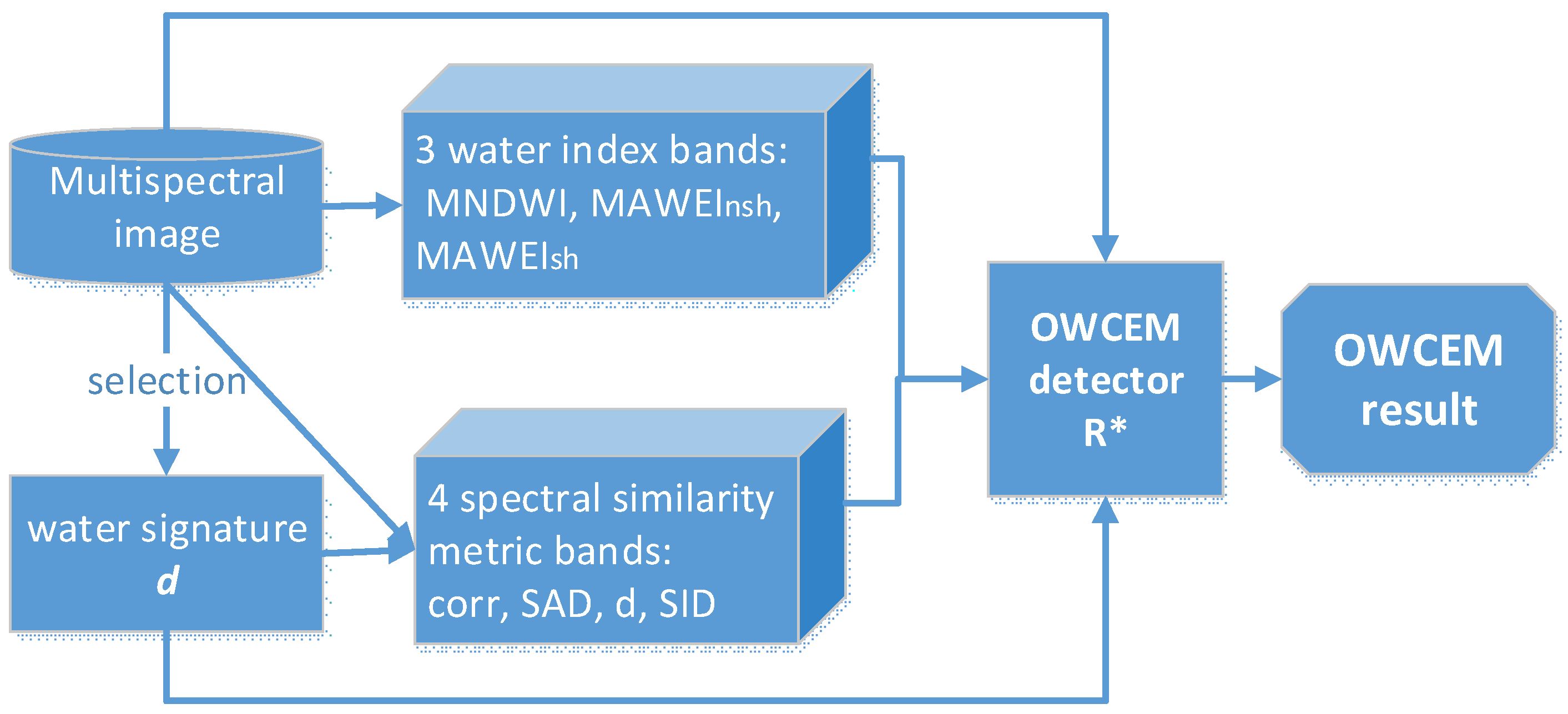
In this study, we compared our method, OWCEM with 14 channels, with the water indices MNDWI, AWEInsh, AWEIsh, and CEM with only the original 7 bands. Strictly speaking, both CEM and OWCEM are detection operators and can be applied to data with any number of channels. However, we simplified OWCEM for “OWCEM applied to 14 channels (Landsat 8 band 1–7 MNDWI, MAWEInsh, MAWEIsh, corr, SAD, d, and SID)” and CEM for “CEM with original 7 bands (Landsat 8 band 1–7)” in the following content. In addition, the Kappa coefficient and the receiver operating characteristic (ROC) curves were calculated to evaluate the performance of the five algorithms.
4.1. Hala Lake
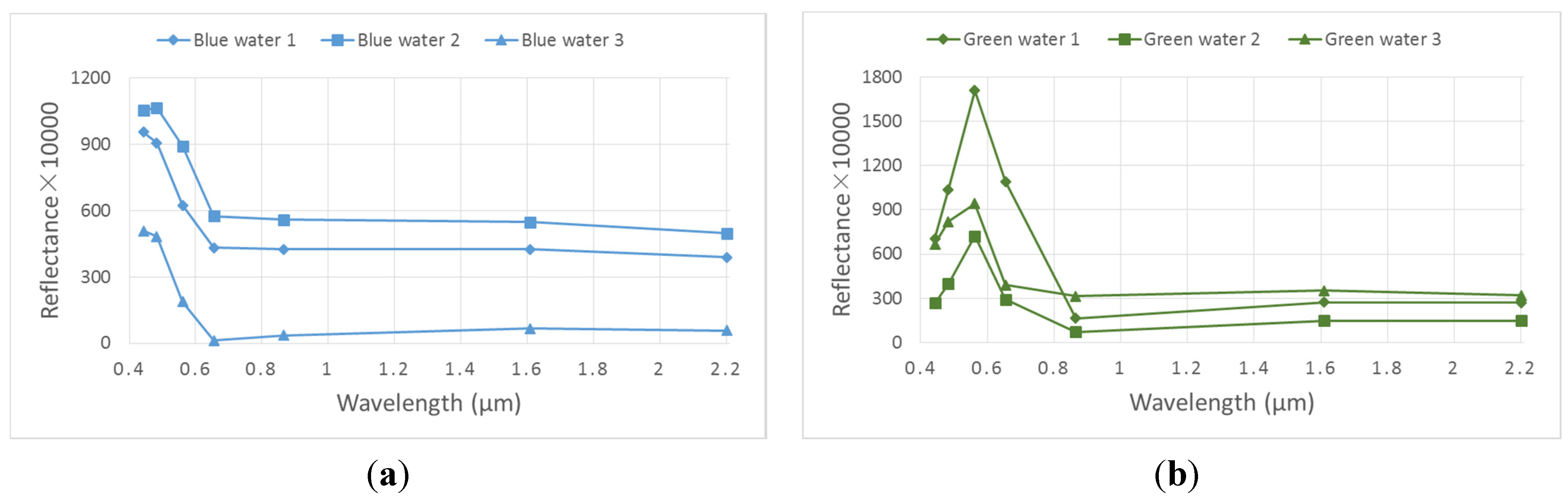
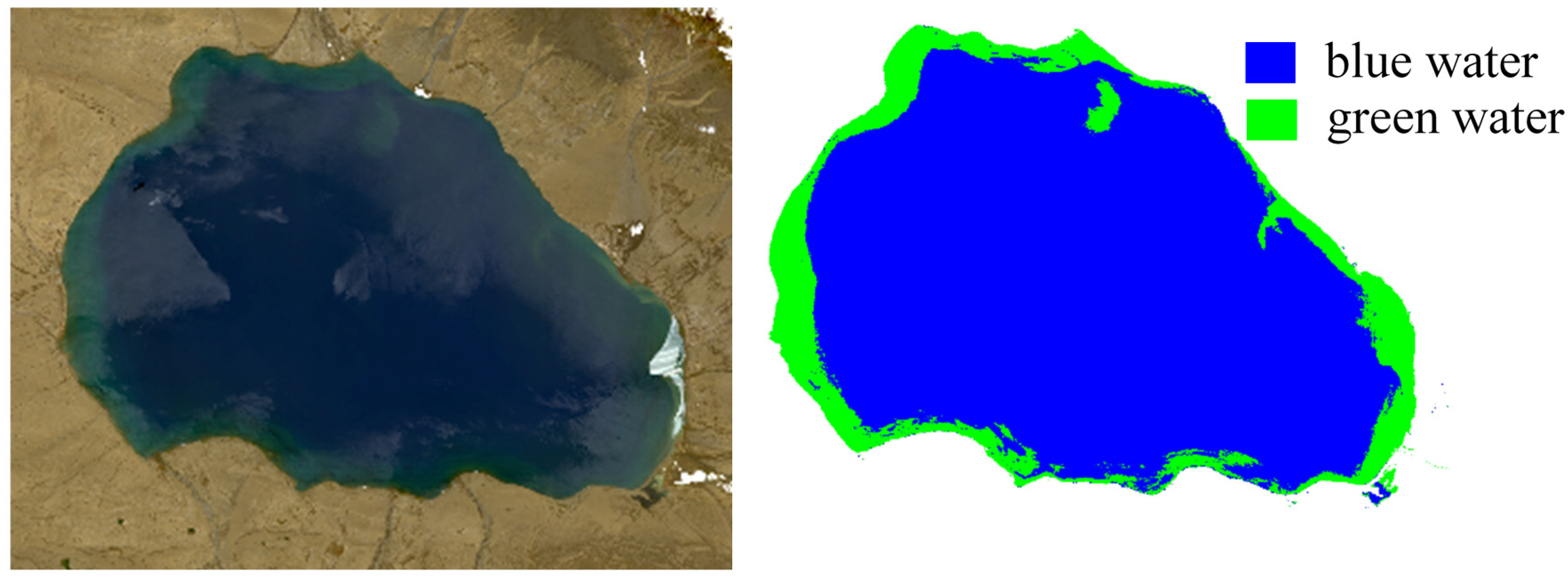
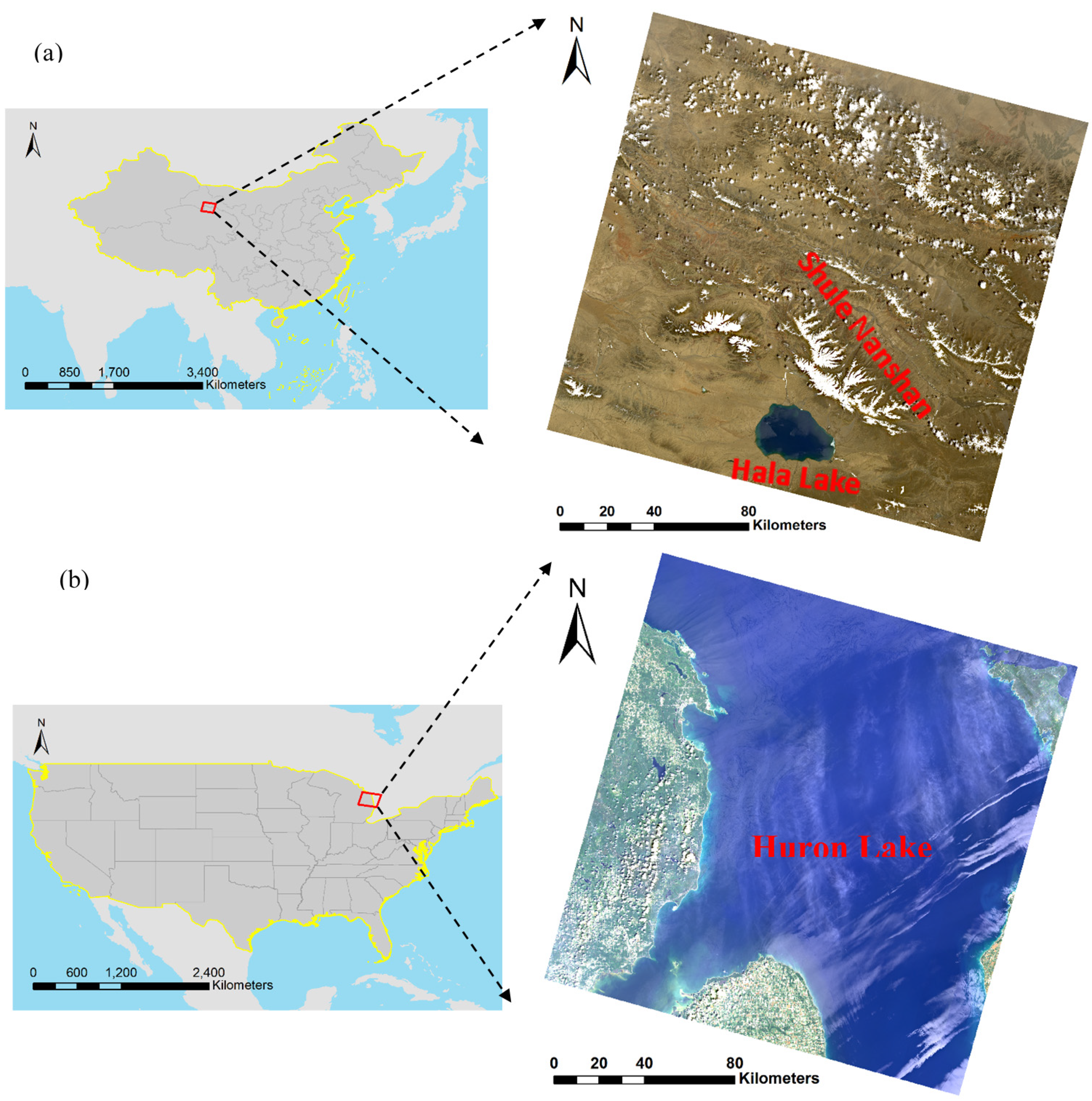
Within the Landsat 8 image, the Hala Lake is a small target, which only occupies 1.57% of the image. However, both ice/snow and cloud exist in the image, as shown in
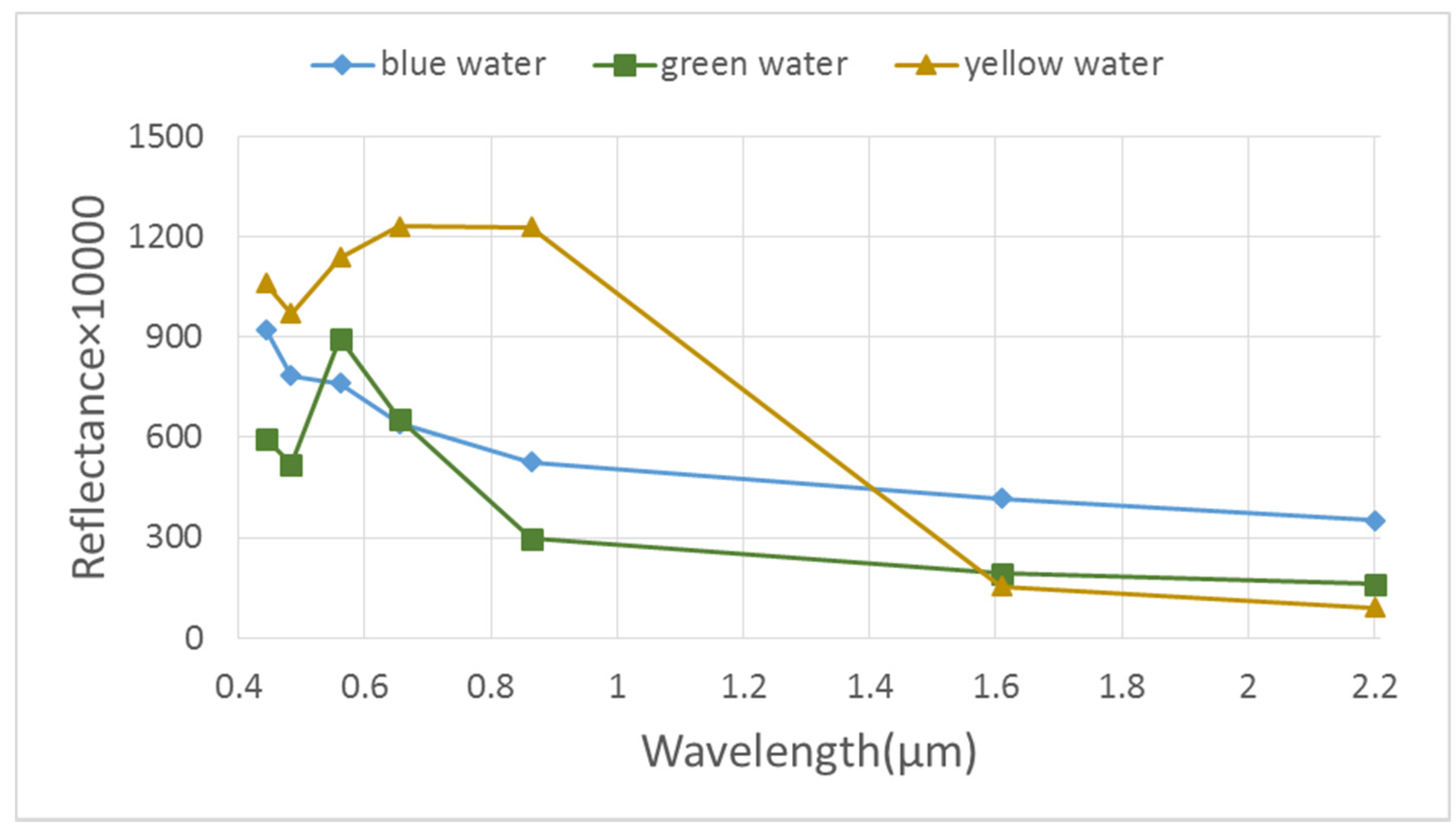
Figure 1a. The middle area of Hala Lake is blue, while some edge areas appear dark green. In this study, three pixels for these two kinds of water were selected as the representatives for CEM and OWCEM, as shown in
Figure 4.
Figure 4.
The spectral curves of blue (a) and green (b) water for the Hala Lake image.
Figure 4.
The spectral curves of blue (a) and green (b) water for the Hala Lake image.
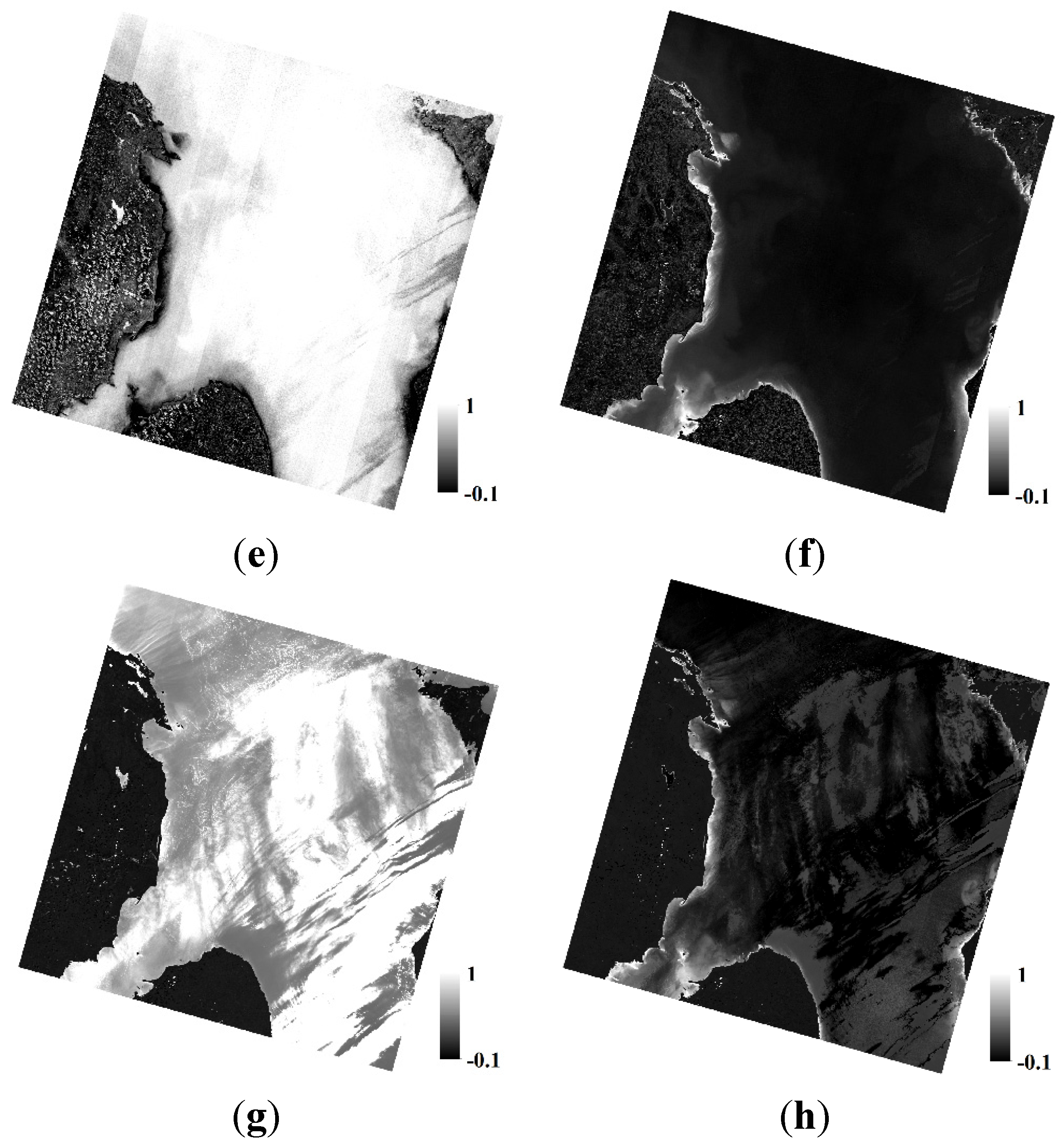
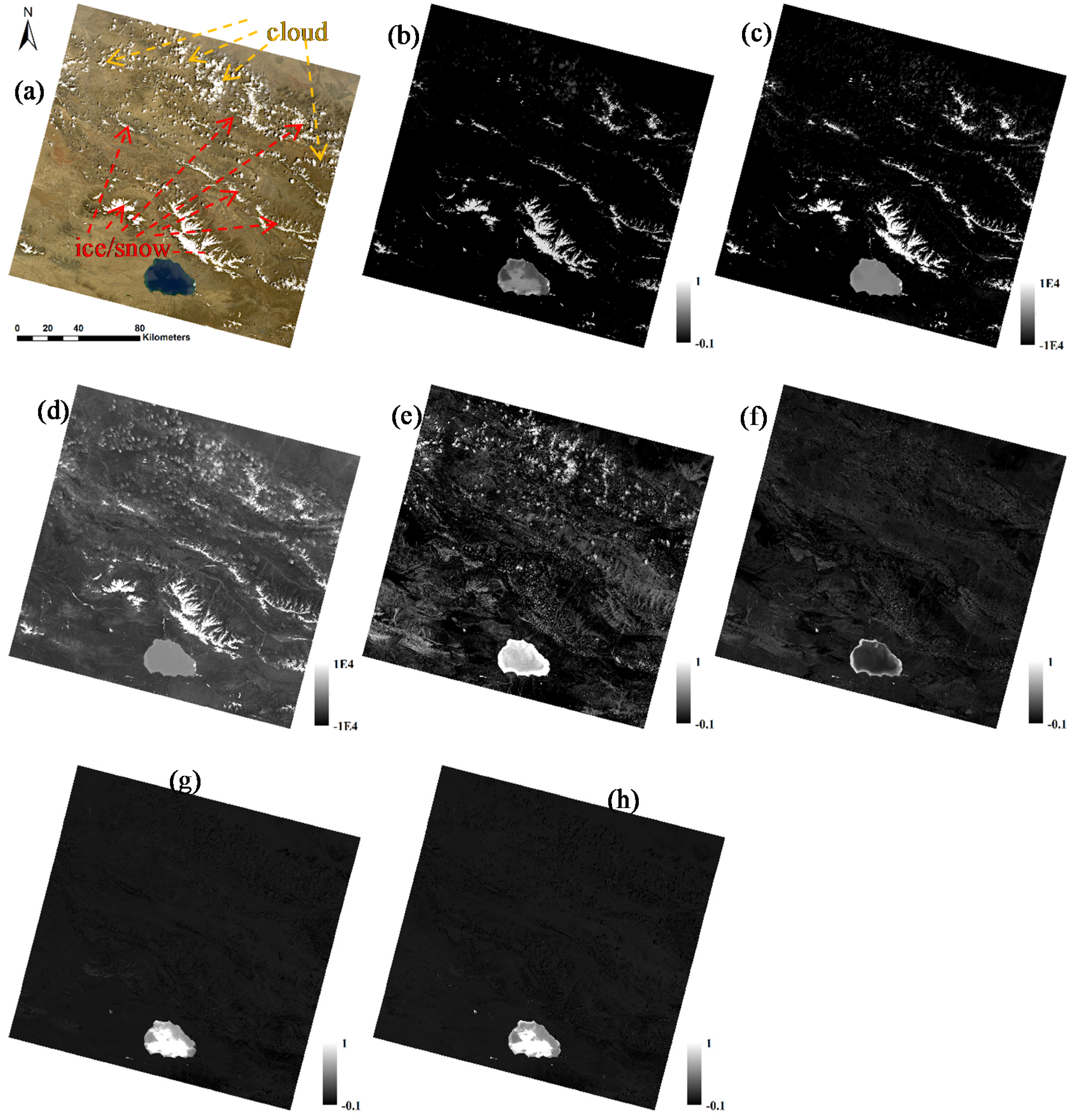
The outputs of the five algorithms are presented in
Figure 5. Visually, OWCEM could suppress the background more efficiently compared to water indices and CEM. Water indices have extremely high values in ice/snow areas (
Figure 5b–d), while CEM has high values in cloudy areas (
Figure 5e). For a quantitative comparison with the ground reference map, the water extraction binary results are required. The most commonly used binarisation is to partition the image by setting a threshold. However, there is no fixed threshold or threshold range for the three published water indices and CEM. For a fair comparison, we adopted the following strategy: first, determine the total number of water pixels from the reference image, denoted as N; second, sort the resulting image (images in
Figure 5) in descending order and mark the first N pixels as water (images in
Figure 6). To extract the whole water area for CEM and OWCEM, we selected the larger value from the results of the blue and green water for each pixel; finally, the ROC curves and Kappa coefficients of all algorithms were generated.
Figure 5.
The results of MNDWI, AWEInsh, AWEIsh, CEM, and OWCEM for blue and green water for the Hala Lake image. (a) True colour image; (b) MNDWI; (c) AWEInsh; (d) AWEIsh; (e) CEM (blue water); (f) CEM (green water); (g) OWCEM (blue water); and (h) OWCEM (green water).
Figure 5.
The results of MNDWI, AWEInsh, AWEIsh, CEM, and OWCEM for blue and green water for the Hala Lake image. (a) True colour image; (b) MNDWI; (c) AWEInsh; (d) AWEIsh; (e) CEM (blue water); (f) CEM (green water); (g) OWCEM (blue water); and (h) OWCEM (green water).
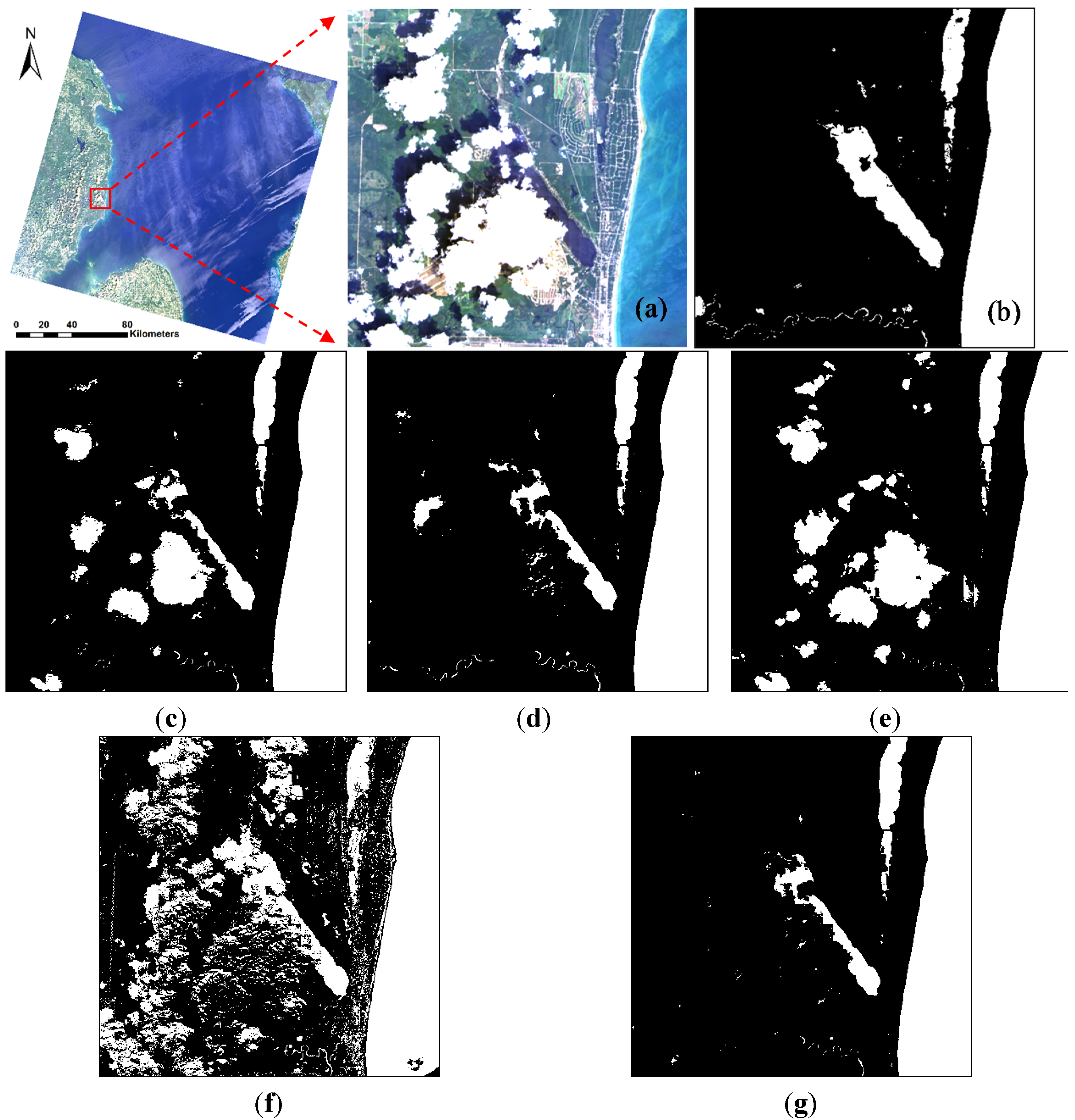
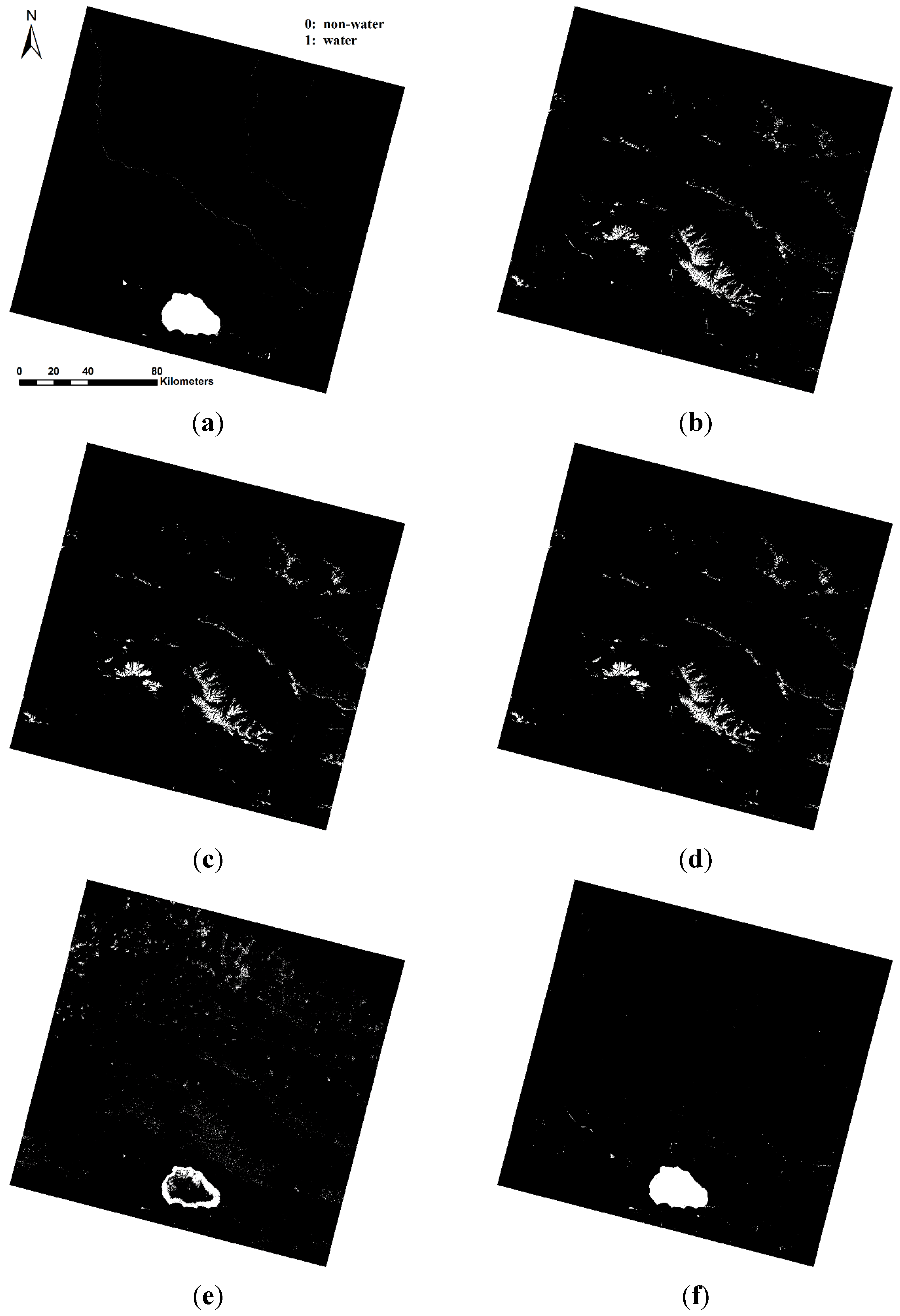
The final water extraction maps for all methods are shown in
Figure 6. A visual comparison indicates that OWCEM produces a better accuracy of water mapping than the water indices and CEM. Only the ice/snow areas are extracted by MNDWI, AWEI
nsh, and AWEI
sh, as shown in
Figure 6b–d. The central part of Hala Lake is missed by CEM, and some ice/snow and cloud areas are extracted by CEM. This is because when extracting blue water, the CEM output shows a higher value in those cloudy and ice/snow areas than those in blue water areas (
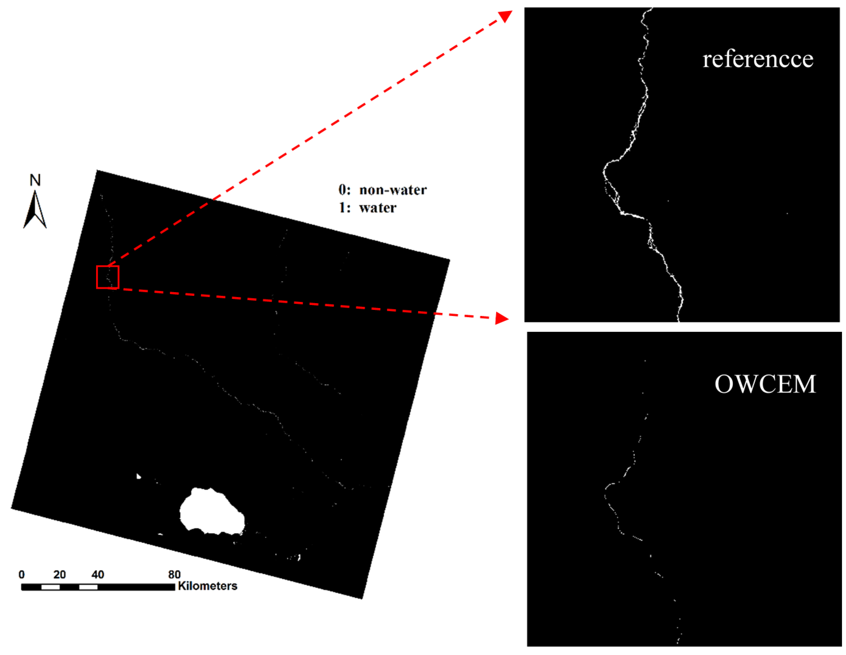
Figure 5e). OWCEM can extract the complete Hala Lake, and some small ponds and rivers around, but no ice/snow or cloudy areas. However, due to the acquisition time difference (refer to
Table 2), there does exist some omissions on small rivers and ponds. For example, the long river across the reference image from the upper-left to the lower-right has not been extracted completely by OWCEM. The corresponding zoom-in images are shown in
Figure 7. The reason for this is that the river water was partially frozen at the acquisition time for the Hala Lake image. Yet, those areas are small, so the Kappa coefficient (see
Table 3) is still very high for OWCEM (0.9647). The Kappa coefficients of MNDWI, AWEI
nsh and AWEI
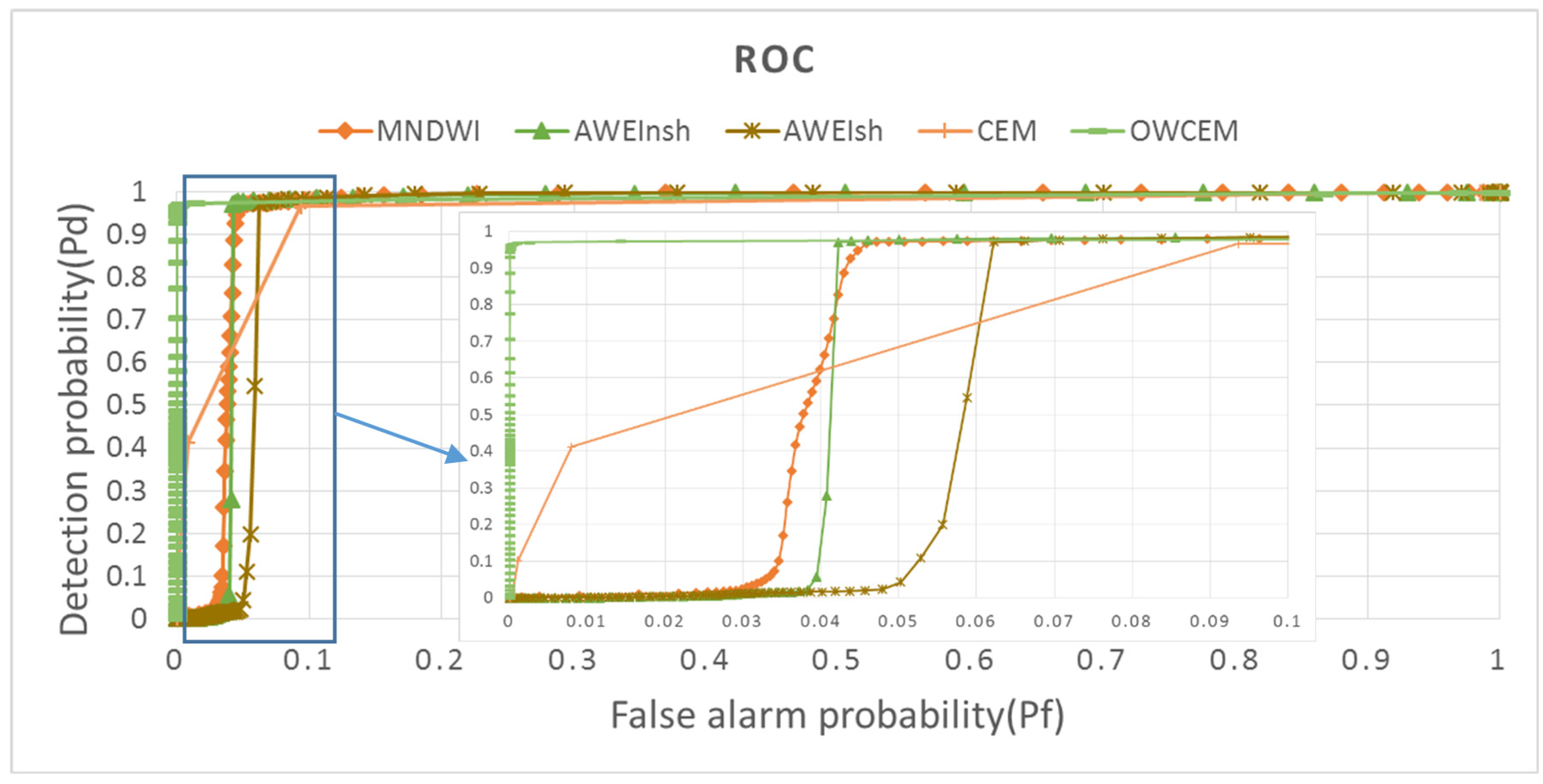
sh are negative, because no water, but only ice/snow and cloud were extracted. The ROC curves of the five methods are shown in
Figure 8. It can be seen that the overall performance of OWCEM is better than that for the other four methods. It yields closely to the (0, 1) of the ROC space, representing OWCEM as an almost perfect classifier.
Figure 6.
Comparison of water extraction results of the five algorithms for Hala Lake image: (a) Reference data; (b) MNDWI; (c) AWEInsh; (d) AWEIsh; (e) CEM; (f) OWCEM.
Figure 6.
Comparison of water extraction results of the five algorithms for Hala Lake image: (a) Reference data; (b) MNDWI; (c) AWEInsh; (d) AWEIsh; (e) CEM; (f) OWCEM.
Figure 7.
Comparison of a subarea of a river in the Hala Lake image between the reference and OWCEM result.
Figure 7.
Comparison of a subarea of a river in the Hala Lake image between the reference and OWCEM result.
Table 3.
The kappa coefficients of the five algorithms for Hala and Lake Huron images.
Table 3.
The kappa coefficients of the five algorithms for Hala and Lake Huron images.
| Classifier | MNDWI | AWEInsh | AWEIsh | CEM | OWCEM |
|---|
| Hala Lake | −0.0076 | −0.0152 | −0.0145 | 0.4744 | 0.9647 |
| Lake Huron | 0.9843 | 0.9843 | 0.9772 | 0.8473 | 0.9928 |
Figure 8.
The ROC curves of the five methods for the Hala Lake image.
Figure 8.
The ROC curves of the five methods for the Hala Lake image.
4.2. Lake Huron
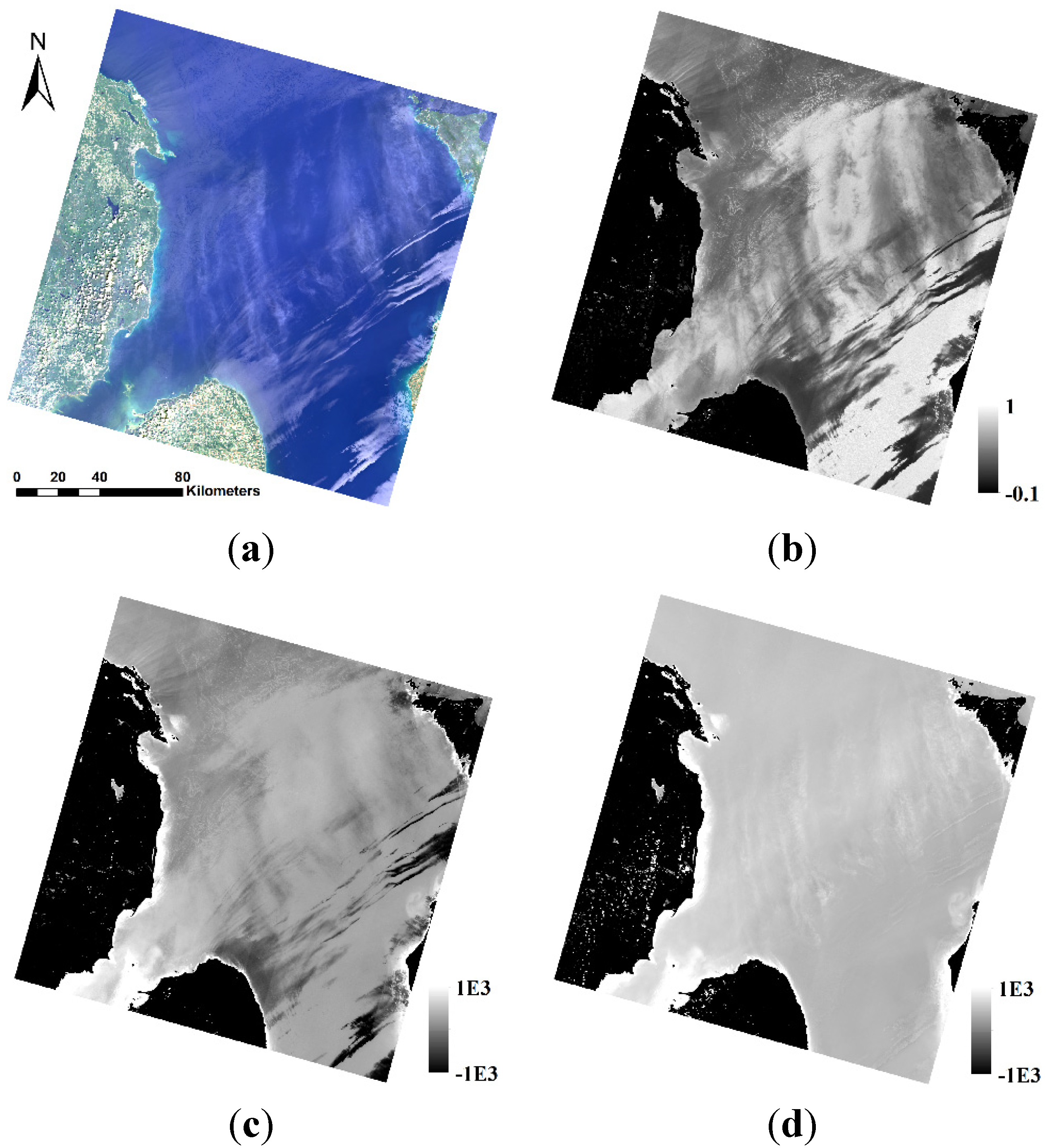
Unlike Hala Lake, Huron Lake occupies the majority of the Landsat 8 image (about 76.4%), as shown in
Figure 1b. In this image, no ice/snow pixels exist. However, thin clouds present on most lake areas, and some thick clouds appear on the land area (
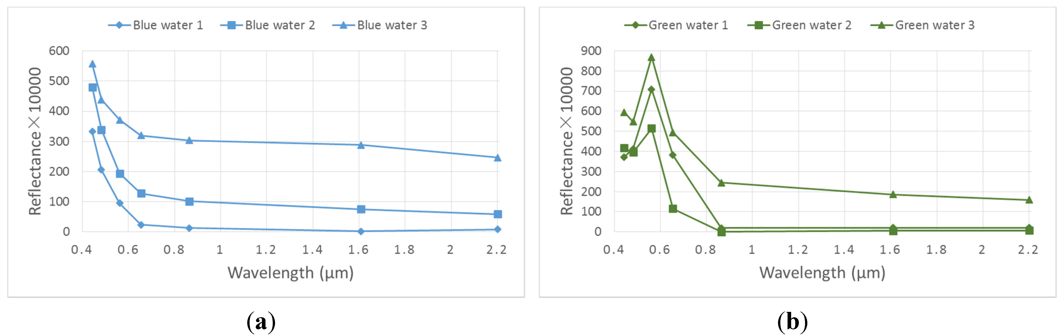
Figure 1b). Most parts of the lake are blue, even when covered by thin cloud. The water at the shore areas appears light green. The signatures of blue and green water selected for
d are shown in
Figure 9.
Figure 9.
The spectral curves of blue (a) and green (b) water for the Lake Huron image.
Figure 9.
The spectral curves of blue (a) and green (b) water for the Lake Huron image.
The results of the five algorithms are presented in
Figure 10. Comparatively speaking, the result of OWCEM shows the strongest contrast between the blue/green water and the background, especially for the blue water. For MNDWI, AWEI
nsh, and AWEI
sh, their combinations of bands have also enhanced the cloud area above land (see
Figure 10b–d)). The CEM result for blue water has the worst contrast effect, because blue water in this image is not a “small target” and only the 7 original bands were used.
Figure 10.
The results of MNDWI, AWEInsh, AWEIsh, CEM, and OWCEM for blue water and OWCEM for green water in the Lake Huron image: (a) True color image; (b) MNDWI; (c) AEWInsh; (d) AWEIsh; (e) CEM (blue); (f) CEM (green); (g) OWCEM (blue); and (h) OWCEM (green).
Figure 10.
The results of MNDWI, AWEInsh, AWEIsh, CEM, and OWCEM for blue water and OWCEM for green water in the Lake Huron image: (a) True color image; (b) MNDWI; (c) AEWInsh; (d) AWEIsh; (e) CEM (blue); (f) CEM (green); (g) OWCEM (blue); and (h) OWCEM (green).
The water extraction procedure is the same as that for Hala Lake, and the results are shown in
Figure 11. MNDWI, AWEI
nsh, and AWEI
sh have all missed some water areas covered by thicker cloud, but extracted some land areas with thick clouds (
Figure 12c–e). CEM has the worst performance. Both cloud and cloud shadow areas on the land part have been extracted by CEM (
Figure 12f). In addition, some water areas near the bank have been missed. The water area extracted by OWCEM is much more complete and even the water areas covered by light cloud have been extracted. However, water covered by very thick cloud cannot be extracted by OWCEM either (
Figure 12g). The kappa coefficients of the five algorithms are tabulated in
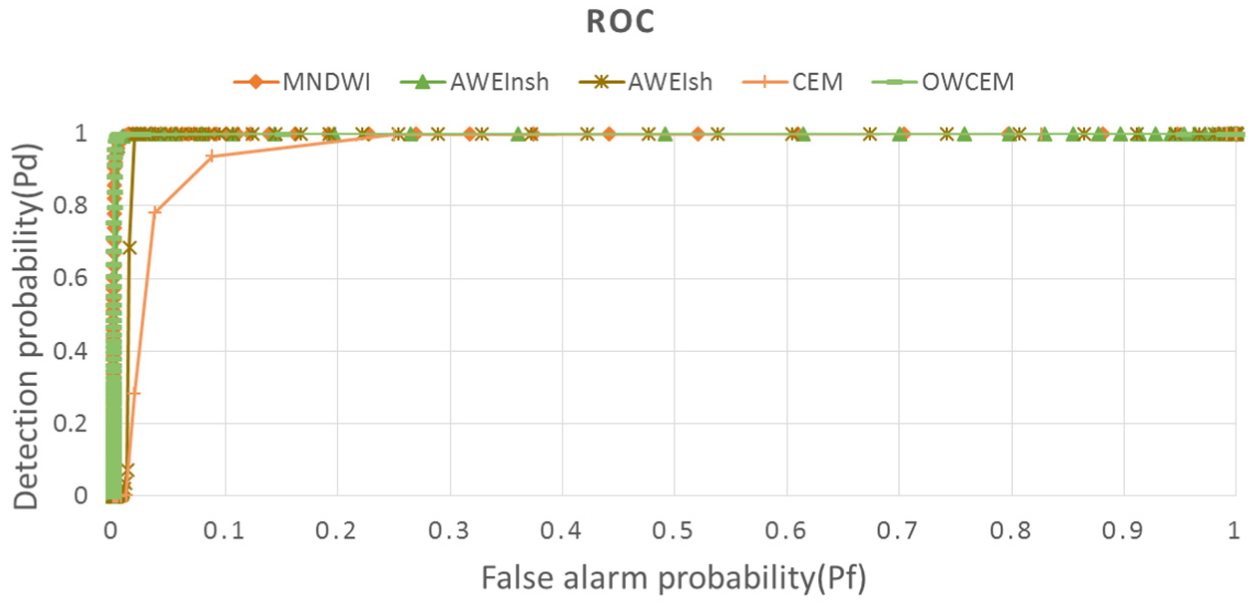
Table 3. OWCEM has the highest value (0.9928) while CEM has the lowest (0.8473). The ROC curves are shown in
Figure 13. The performance of MNDWI is very close to that of OWCEM. Overall, OWCEM still performs best, even though the percentage of water is very large in the image. To further investigate the influence of target size on CEM, we applied CEM to the 14-channel data. The corresponding kappa coefficient became even lower (0.3290), which again indicates that CEM has poor performance for a large size targets, and may perform worse when more data is added. The main reason for this is that the autocorrelation matrix
R of this image used in the CEM detector mostly represents the statistical information on water, not the background. By introducing a weight when constructing the autocorrelation matrix, OWCEM has no limit on target size.
Figure 11.
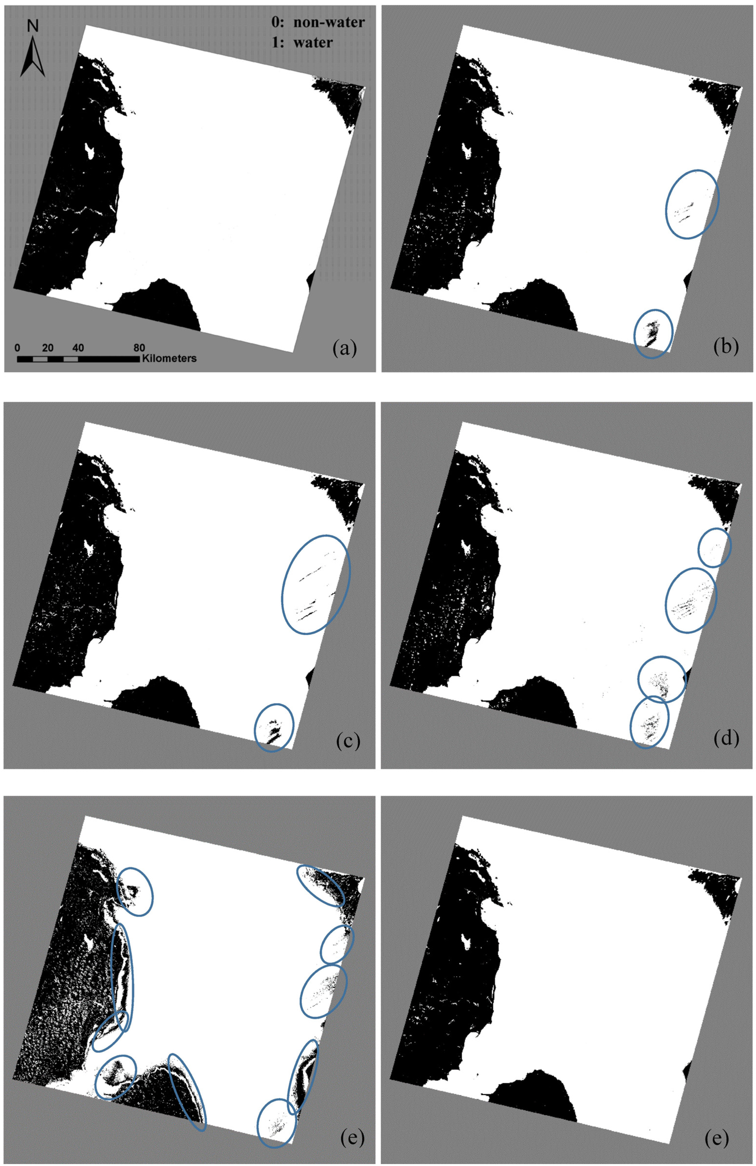
Comparison of water extraction results of the five algorithms for the Lake Huron image. Areas in circles indicate the missing water areas. (a) Reference data; (b) MNDWI; (c) AWEInsh; (d) AWEIsh; (e) CEM; and (f) OWCEM.
Figure 11.
Comparison of water extraction results of the five algorithms for the Lake Huron image. Areas in circles indicate the missing water areas. (a) Reference data; (b) MNDWI; (c) AWEInsh; (d) AWEIsh; (e) CEM; and (f) OWCEM.
Figure 12.
Details of water extraction results using the five algorithms for the Lake Huron image: (a) True colour image; (b) reference; (c) MNDWI; (d) AWEInsh; (e) AWEIsh; (f) CEM; and (g) OWCEM.
Figure 12.
Details of water extraction results using the five algorithms for the Lake Huron image: (a) True colour image; (b) reference; (c) MNDWI; (d) AWEInsh; (e) AWEIsh; (f) CEM; and (g) OWCEM.
Figure 13.
The ROC curves of the five algorithms for the Lake Huron image.
Figure 13.
The ROC curves of the five algorithms for the Lake Huron image.
4.3. Analysis on Correlation between Channels
The above results on the two lakes indicate that adding water index and spectral similarity metric channels in OWCEM can greatly improve the accuracy of water mapping.
Table 4 and
Table 5 tabulate the correlation coefficients between the 7 additional channels and all 14 channels used in the Hala Lake and Lake Huron images. We find that the correlation coefficients between the water indices, and the correlation coefficients between corr, SAD, and SID are high. Also, the d channel has a high correlation with the VNIR (visible and near-infrared) bands. To assess the influence of the channel correlation to the result of OWCEM, we conducted a comparison study by adding (1) a zero mean Gaussian distributed random noise with a standard deviation of one, denoted as
n1; (2) an existing channel disturbed by a small Gaussian distributed random noise with a mean of zero and a standard deviation of 0.0001, denoted as n
2; and (3) a water index/spectral similarity metric.
Table 4.
The correlation coefficient matrix for the data set used in the Hala Lake image.
Table 4.
The correlation coefficient matrix for the data set used in the Hala Lake image.
| Channel | MNDWI | MAWEInsh | MAWEIsh | corr | SAD | d | SID | n1 | MADWI + n2 | Corr + n2 |
|---|
| B1 | 0.8092 | 0.7894 | 0.6789 | 0.7224 | −0.7271 | 0.9281 | −0.5889 | −0.0003 | 0.8092 | 0.7224 |
| B2 | 0.8028 | 0.7821 | 0.6678 | 0.7107 | −0.7214 | 0.9365 | −0.5873 | −0.0003 | 0.8028 | 0.7107 |
| B3 | 0.7612 | 0.7349 | 0.6100 | 0.6526 | −0.6973 | 0.9624 | −0.5815 | −0.0003 | 0.7612 | 0.6526 |
| B4 | 0.7027 | 0.6726 | 0.5408 | 0.5797 | −0.6578 | 0.9755 | −0.5622 | −0.0003 | 0.7027 | 0.5797 |
| B5 | 0.5568 | 0.5293 | 0.3927 | 0.4341 | −0.5592 | 0.9773 | −0.4983 | −0.0002 | 0.5568 | 0.4341 |
| B6 | −0.4072 | −0.4587 | −0.4006 | −0.4457 | 0.0447 | 0.3687 | −0.1337 | −0.0001 | −0.4072 | −0.4457 |
| B7 | −0.3466 | −0.4085 | −0.3409 | −0.3981 | −0.0032 | 0.4068 | −0.1828 | −0.0001 | −0.3466 | −0.3981 |
| MNDWI | 1.0000 | 0.9934 | 0.9380 | 0.9135 | −0.8212 | 0.6131 | −0.6612 | −0.0002 | 1.0000 | 0.9135 |
| MAWEInsh | 0.9934 | 1.0000 | 0.9430 | 0.9179 | −0.7834 | 0.5758 | −0.6059 | −0.0002 | 0.9934 | 0.9179 |
| MAWEIsh | 0.9380 | 0.9430 | 1.0000 | 0.8907 | −0.7662 | 0.4877 | −0.6228 | −0.0003 | 0.9380 | 0.8907 |
| Corr | 0.9135 | 0.9179 | 0.8907 | 1.0000 | −0.7217 | 0.5031 | −0.5101 | −0.0002 | 0.9135 | 1.0000 |
| SAD | −0.8212 | −0.7834 | −0.7662 | −0.7217 | 1.0000 | −0.6286 | 0.9010 | 0.0002 | −0.8212 | −0.7217 |
| d | 0.6131 | 0.5758 | 0.4877 | 0.5031 | −0.6286 | 1.0000 | −0.5740 | −0.0003 | 0.6131 | 0.5031 |
| SID | −0.6612 | −0.6059 | −0.6228 | −0.5101 | 0.9010 | −0.5740 | 1.0000 | 0.0002 | −0.6612 | −0.5101 |
Table 5.
The correlation coefficient matrix for the data set used in the Lake Huron image.
Table 5.
The correlation coefficient matrix for the data set used in the Lake Huron image.
| Channel | MNDWI | MAWEInsh | MAWEIsh | Corr | SAD | d | SID | n1 | MNDWI + n2 | Corr + n2 |
|---|
| B1 | −0.1217 | −0.1842 | −0.1519 | −0.1056 | −0.0199 | 0.8368 | −0.0299 | −0.0001 | −0.1217 | −0.1056 |
| B2 | −0.1539 | −0.2128 | −0.1824 | −0.1368 | 0.0046 | 0.8543 | −0.0015 | −0.0001 | −0.1539 | −0.1368 |
| B3 | −0.3625 | −0.3824 | −0.3705 | −0.3655 | 0.2165 | 0.9321 | 0.2241 | 0.0001 | −0.3625 | −0.3655 |
| B4 | −0.3316 | −0.3677 | −0.3371 | −0.3445 | 0.1875 | 0.9282 | 0.1787 | 0.0000 | −0.3316 | −0.3445 |
| B5 | −0.8559 | −0.7331 | −0.7715 | −0.8981 | 0.8484 | 0.7830 | 0.8754 | 0.0004 | −0.8559 | −0.8981 |
| B6 | −0.7625 | −0.6909 | −0.6890 | −0.8210 | 0.7032 | 0.9015 | 0.7106 | 0.0004 | −0.7624 | −0.8210 |
| B7 | −0.6181 | −0.5957 | −0.5680 | −0.6761 | 0.5204 | 0.9464 | 0.5097 | 0.0002 | −0.6181 | −0.6761 |
| MNDWI | 1.0000 | 0.9547 | 0.9690 | 0.8948 | −0.8303 | −0.5075 | −0.8658 | −0.0005 | 1.0000 | 0.8948 |
| MAWEInsh | 0.9547 | 1.0000 | 0.9851 | 0.7579 | −0.6469 | −0.4524 | −0.6802 | −0.0004 | 0.9547 | 0.7579 |
| MAWEIsh | 0.9690 | 0.9851 | 1.0000 | 0.7743 | −0.6782 | −0.4427 | −0.7359 | −0.0005 | 0.9690 | 0.7743 |
| Corr | 0.8948 | 0.7579 | 0.7743 | 1.0000 | −0.9578 | −0.5923 | −0.9322 | −0.0005 | 0.8948 | 1.0000 |
| SAD | −0.8303 | −0.6469 | −0.6782 | −0.9578 | 1.0000 | 0.4879 | 0.9730 | 0.0005 | −0.8303 | −0.9578 |
| d | −0.5075 | −0.4524 | −0.4427 | −0.5923 | 0.4879 | 1.0000 | 0.4676 | 0.0002 | −0.5075 | −0.5923 |
| SID | −0.8658 | −0.6802 | −0.7359 | −0.9322 | 0.9730 | 0.4676 | 1.0000 | 0.0005 | −0.8658 | −0.9322 |
The resulting kappa coefficients are listed in
Table 6. Though n
1 has very low correlation with the other channels (see
Table 4 and
Table 5), the kappa coefficient is not increased when added. This is a consequence of the fact that n
1 contains little useful information. On the other hand, adding MNDWI +
n2 and corr +
n2, which are highly correlated with MNDWI and corr, respectively, will be of no benefit in improving performance either, because those channels have no extra information. However, when the other water index/spectral similarity metric channel is added, the kappa coefficient increased, as shown in
Table 6. For example, adding d can further increase the kappa coefficient, although it has a high correlation with the VNIR bands. Therefore, only adding data with extra useful information can improve the performance of OWCEM. This useful information is derived from people’s physical understanding of the target. For example, the water indices added in this paper contain people’s empirical knowledge about the spectral characteristics of the water.
Table 6.
The kappa coefficients for different combinations of channels used in OWCEM.
Table 6.
The kappa coefficients for different combinations of channels used in OWCEM.
| Data used for OWCEM | Hala Lake | Lake Huron |
|---|
| 7 Landsat bands, MNDWI | 0.8024 | 0.9428 |
| 7 Landsat bands, MNDWI, n1 | 0.8024 | 0.9428 |
| 7 Landsat bands, MNDWI, MNDWI + n2 | 0.8022 | 0.9427 |
| 7 Landsat bands, MNDWI, MAWEIsh | 0.9638 | 0.9761 |
| 7 Landsat bands, MNDWI, MAWEIsh, d | 0.9640 | 0.9916 |
| 7 Landsat bands, corr | 0.5505 | 0.9907 |
| 7 Landsat bands, corr, n1 | 0.5500 | 0.9907 |
| 7 Landsat bands, corr, corr + n2 | 0.5501 | 0.9907 |
| 7 Landsat bands, corr, SAD | 0.9263 | 0.9927 |
5. Discussion and Perspectives
From the results at Hala and Huron Lakes, we find that water indices are more sensitive to ice/snow while CEM is more sensitive to cloud. OWCEM has a better suppression effect on both snow/ice and clouds. From the spectral curves of water and ice/snow, it can be observed that the SWIR bands of both water and ice/snow have a lower reflectance compared to the VIS and NIR bands. Thus, to some extent, there does exist some similarity between water and ice/snow. However, ice/snow has a much higher reflectance value than water. Therefore, adding Euclidean distance data could help OWCEM to distinguish water from ice/snow. The spectral signature for thin cloud is much more complicated, which usually varies as the ground objects below change. Therefore, it is hard to say which specific additional channel plays a more important role for OWCEM to suppress cloud. We think all additional channels make some contribution. For example, from
Figure 5 and
Figure 10 we can see that both MNDWI and AWEI
nsh have a better suppression effect on cloud than CEM, although this is not particularly obvious.
Another advantage of our algorithm is that OWCEM is less sensitive to the selection for
d than CEM. Both OWCEM and CEM use the same pixels for calculating
ds, but CEM has missed some water areas in results of both lakes (see
Figure 6e and
Figure 11e). This implies that a target pixel with a slightly different signature in shape or value from the desired signature d may be considered as an undesirable or background pixel by CEM. However, the situation for OWCEM is much better. This is because the additional water indices can enhance the information for all water types, thus lowering the impact caused by the spectral differences in the original bands between waters. In practical applications, the most representative water samples should be selected for OWCEM for better performance.
Therefore, regardless of the distribution of the target, the main advantage for OWCEM outperforming CEM is the added channels. Suitable additional data could help OWCEM to avoid the drawbacks of CEM in many aspects. From the above analysis, we can conclude that data which both reflects the common characteristics of various water types and that highlights the difference between water to background should be included in OWCEM. In this study, we only show one combination of added channels, and the result is encouraging. Thus, other useful information could also be tried in the future, such as shape information, texture, etc.
OWCEM is a supervised classifier, which requires water training samples as input. In fact, the ground truth maps are generated using the support vector machine (SVM) classifier by selecting samples for 11 level-1 and 28 level-2 land cover types, including water, ice, snow and clouds,
etc. From the comparison results between OWCEM and the reference maps, we can see that the performance of our algorithm is comparable to that of SVM. However, OWCEM requires much less prior knowledge on samples, which could therefore save a lot of time in sample selection and adjustment. Moreover, OWCEM outputs are also suitable for the classification of water types by setting a different
d value for different kinds of water. Taking Hala Lake as an example, by classifying the water types by choosing a larger OWCEM value, we can get a water-type map of Hala Lake, as shown in
Figure 14.
Figure 14.
The classification result of Hala Lake by OWCEM.
Figure 14.
The classification result of Hala Lake by OWCEM.
In addition, it should be pointed out here that the water map in
Figure 6 and
Figure 11 are extracted by the new strategy to achieve a fair comparison. However, people tend to use threshold segmentation or other classifiers for further water extraction. Here, we computed two different indices, the separability index (SI) [
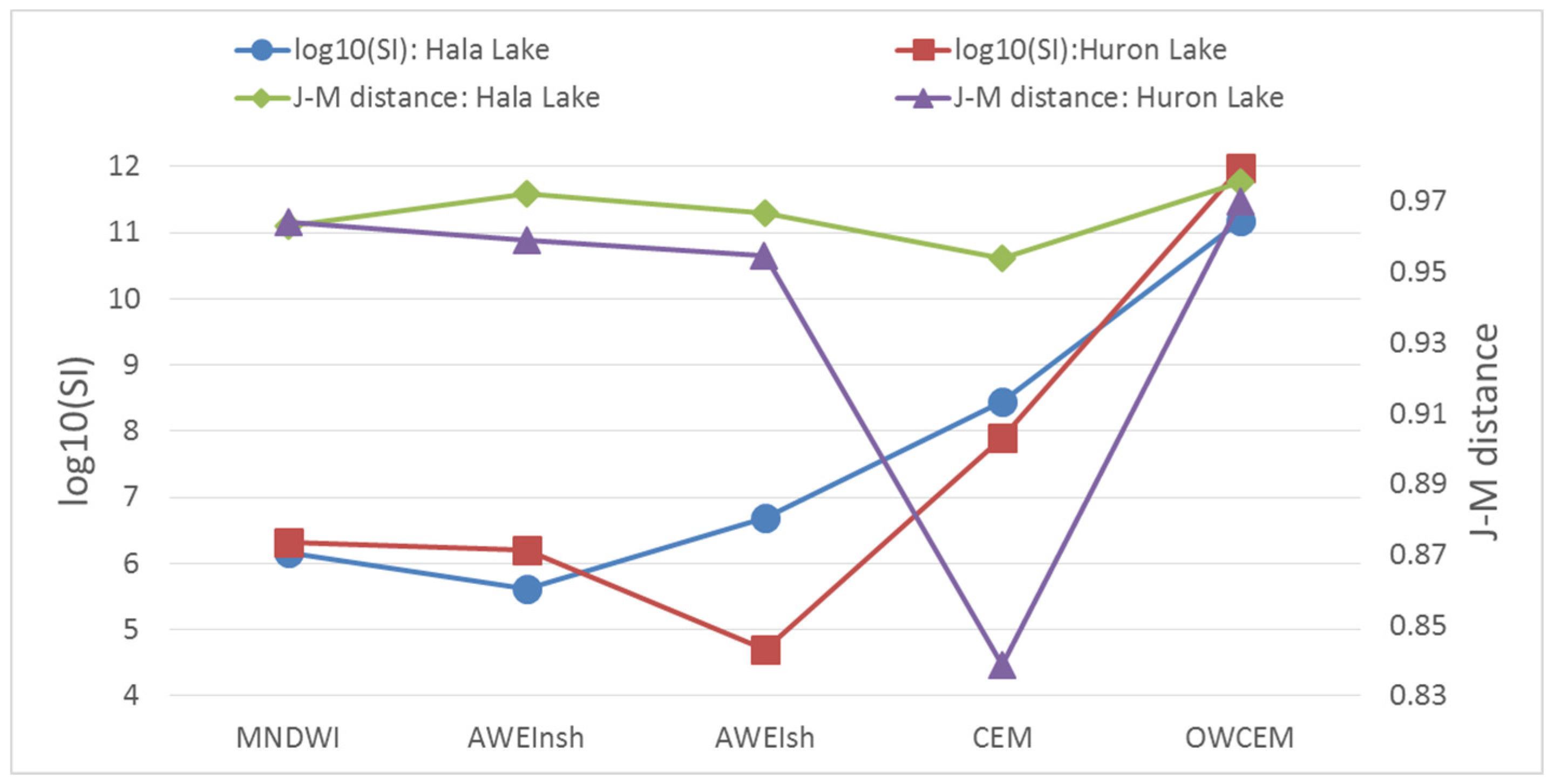
42] and the Jeffries–Matusita (J–M) distance, to measure the degree of separation between the target and the background. From
Figure 15, we can see that OWCEM has the highest value in both indices, which indicates that water and non-water area are more easily separable with the OWCEM result than with the other four. The values from OWCEM usually range between −1 and 1. The threshold value can be determined automatically or manually. Through multiple tries, we found that OWCEM could achieve a stable threshold range. For these two tests, the suitable threshold is around 0.3.
Figure 15.
The SI and J–M distance of the five algorithms.
Figure 15.
The SI and J–M distance of the five algorithms.


