
Target Detection Method for Water Mapping Using Landsat 8 OLI/TIRS Imagery

Abstract
:1. Introduction
2. Study Areas and Data Source
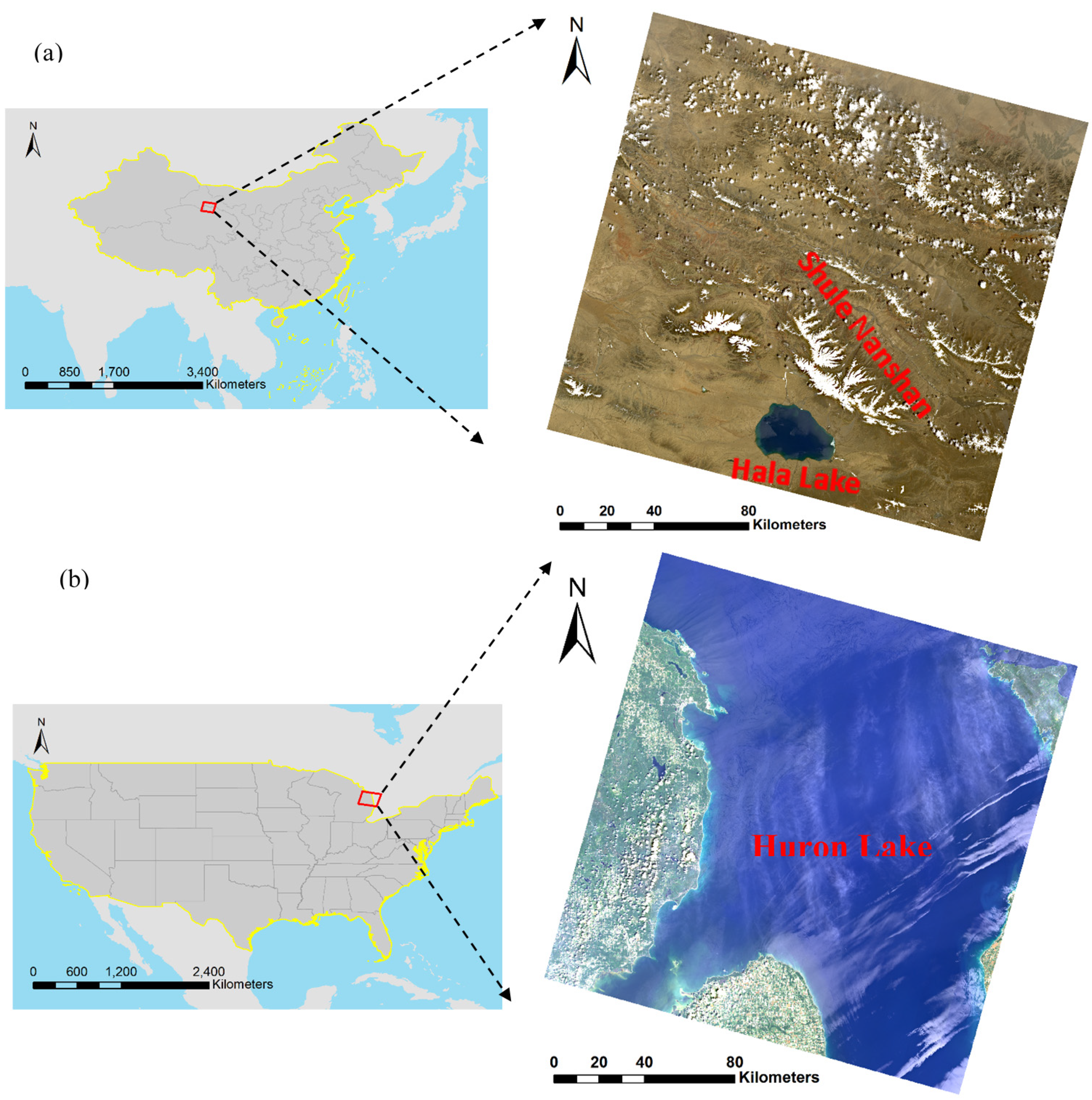
2.1. Test Sites
2.2. Landsat Images

| Sensor | Bands | ||||||||||
|---|---|---|---|---|---|---|---|---|---|---|---|
| Costal Aerosol | Blue | Green | Red | NIR | SWIR 1 | SWIR 2 | Panchromatic | Cirrus | TIRS 1 | TIRS 2 | |
| TM | - | 1 | 2 | 3 | 4 | 5 | 7 | - | - | 6 | |
| ETM+ | - | 1 | 2 | 3 | 4 | 5 | 7 | 8 | - | 6 | |
| OLI/TIRS | 1 | 2 | 3 | 4 | 5 | 6 | 7 | 8 | 9 | 10 | 11 |
| Test Site | Path/Row | Central Latitude/Longitude | Acquisition Date | Image Size | Cloud Cover | Water Cover | Reference Data |
|---|---|---|---|---|---|---|---|
| Hala Lake | 135/033 | 38°89' N/97°69' E | 01/06/2013 | 7691/7501 | 5.08% | 1.75% | FROM-GLC: base image acquired on 09/08/2009 |
| Huron Lake | 020/029 | 44°59' N/82°71' W | 13/07/2013 | 7901/8021 | 1.29% | 76.40% | FROM-GLC: base image acquired on 20/09/2009 |
2.3. Reference Data
3. Methods
3.1. CEM
3.2. Band Expansion
3.2.1. Water Index
3.2.2. Spectral Similarity Metrics
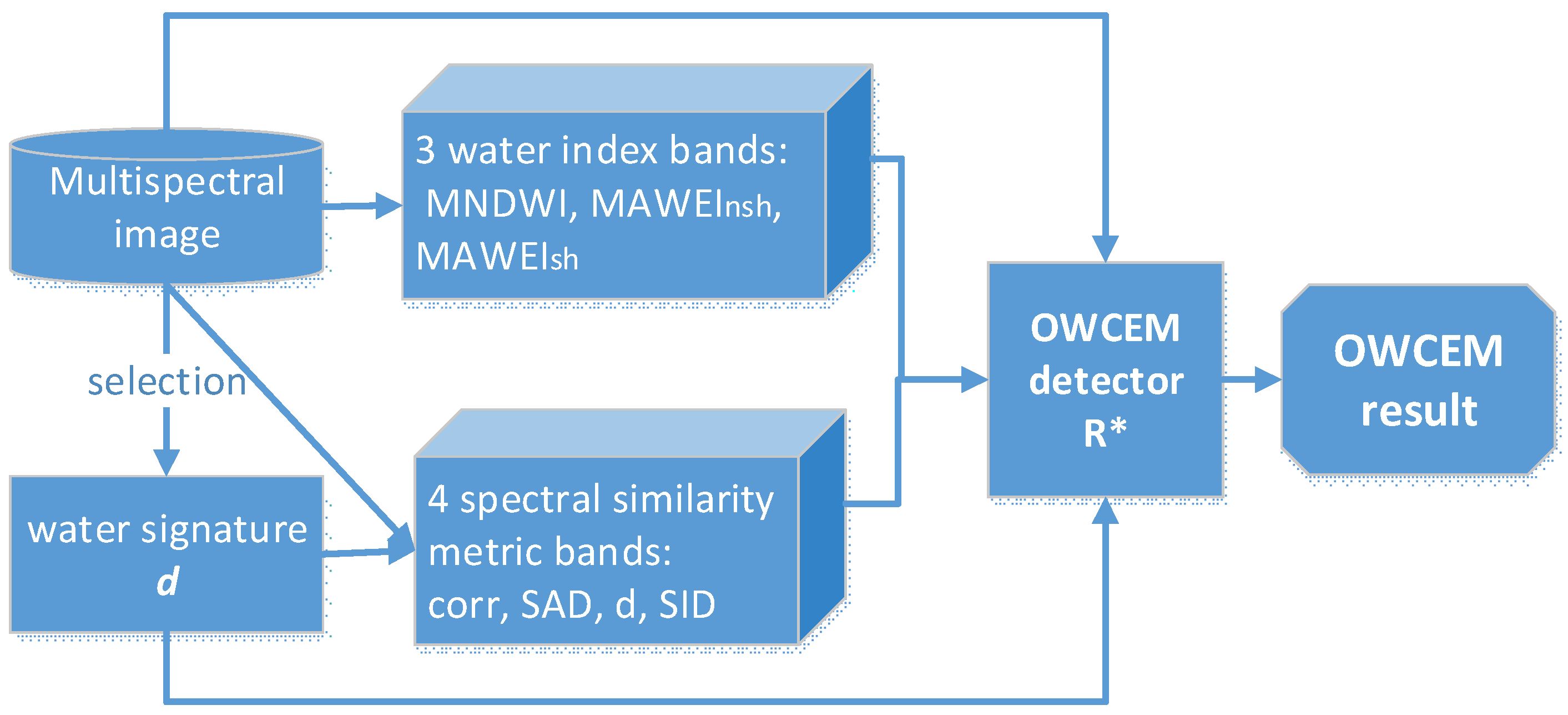
3.3. CEM Based on Orthogonal Subspace Projection-Weighted Autocorrelation Matrix

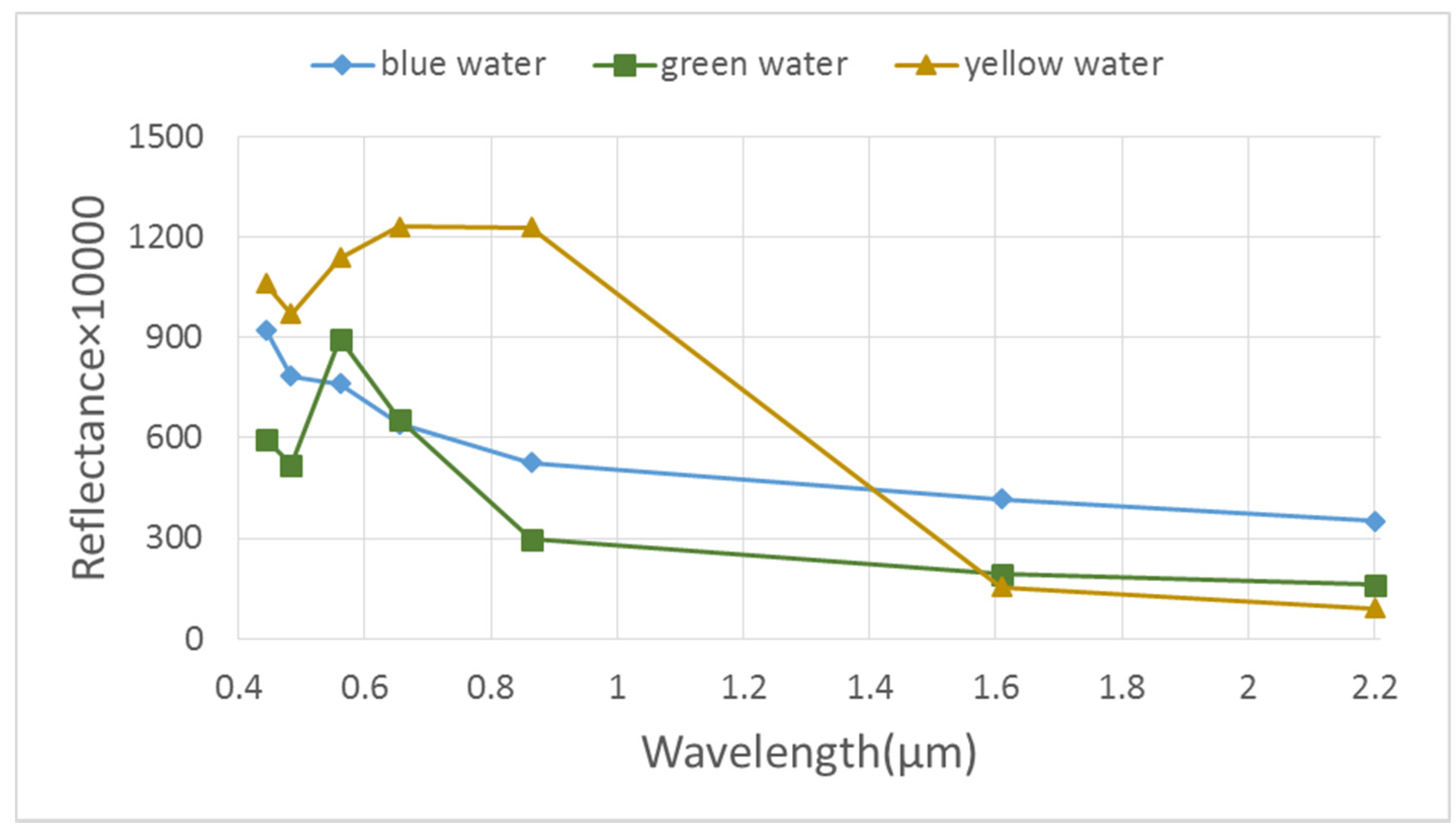
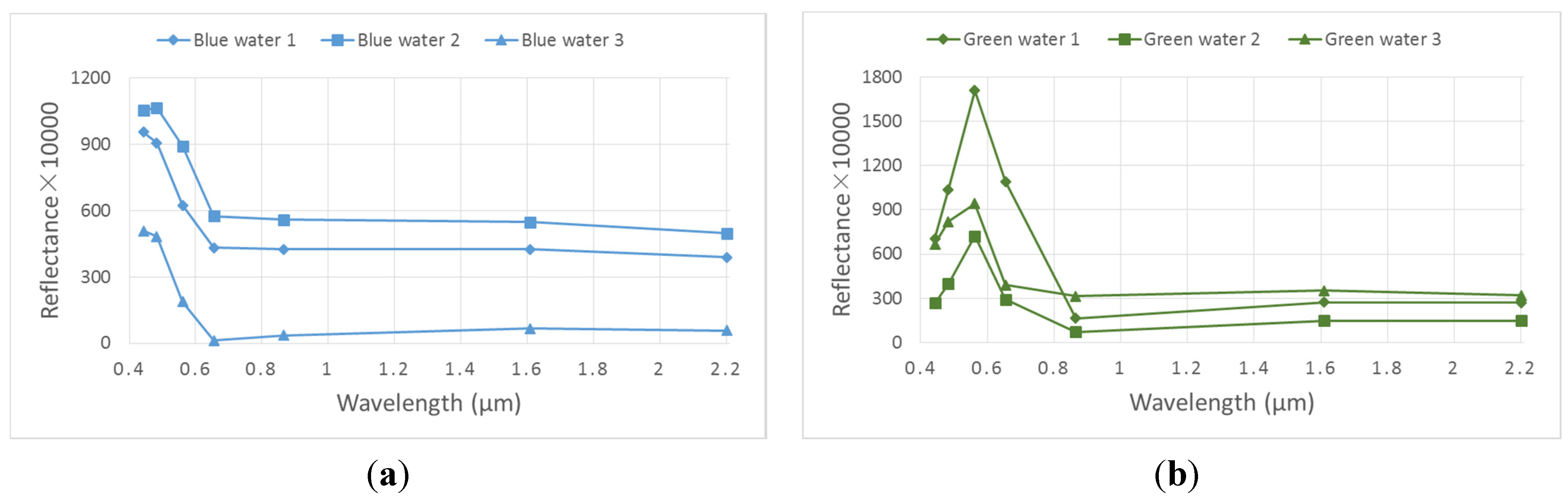
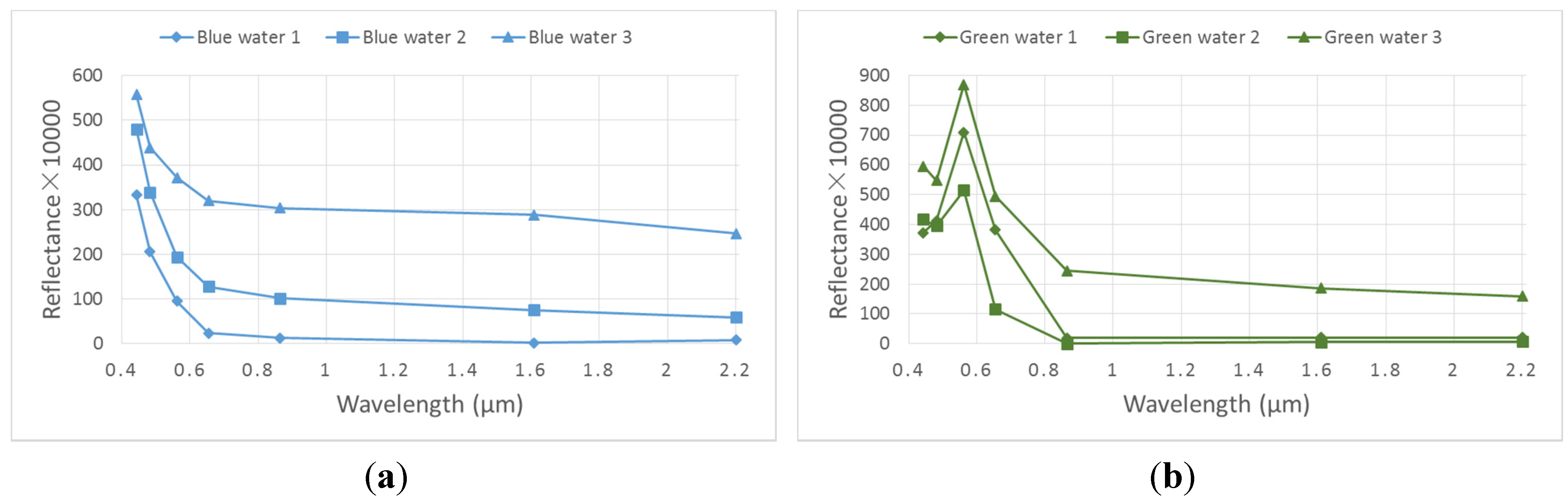
3.4. Pure Water Signature Extraction

4. Results
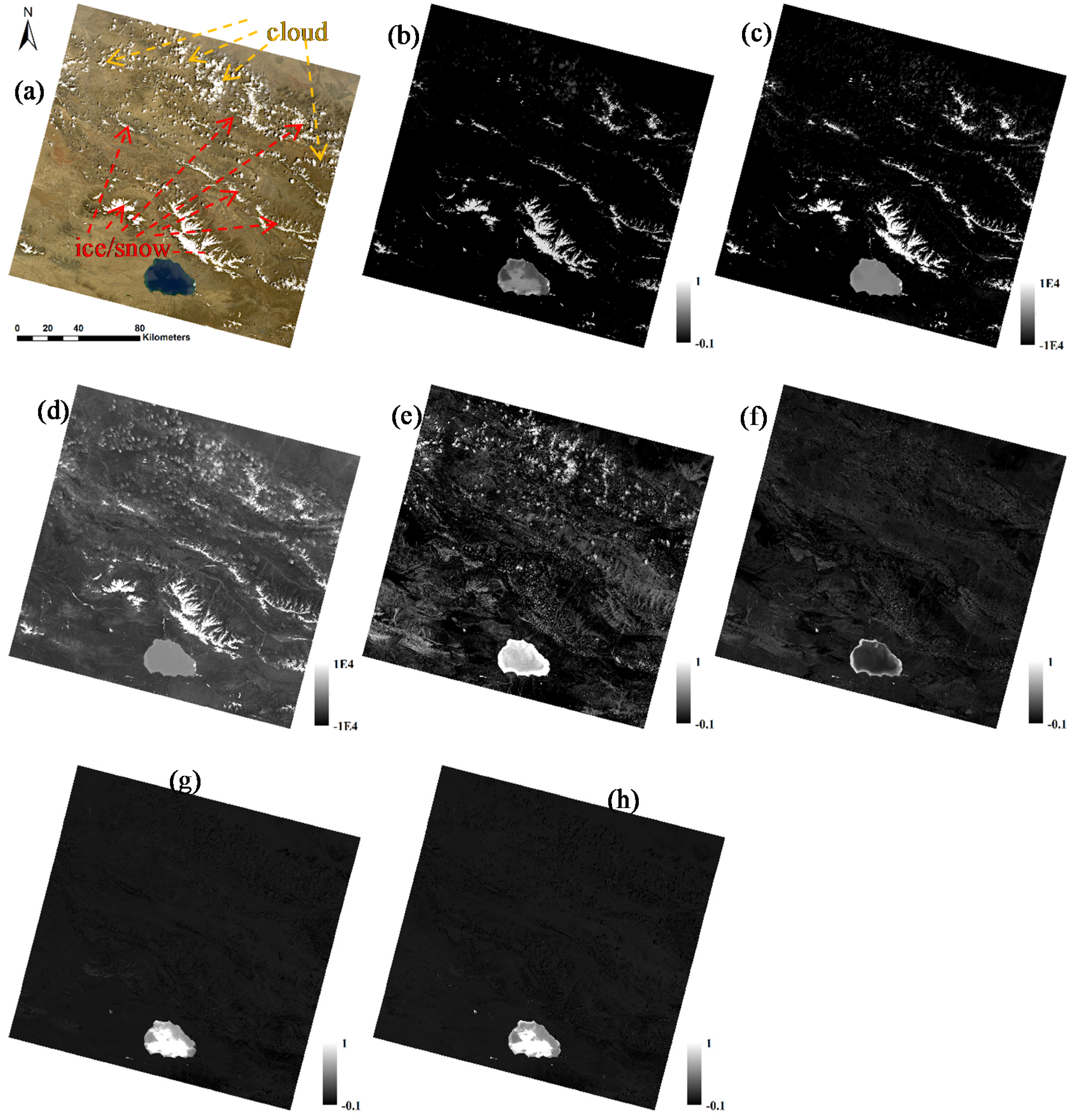
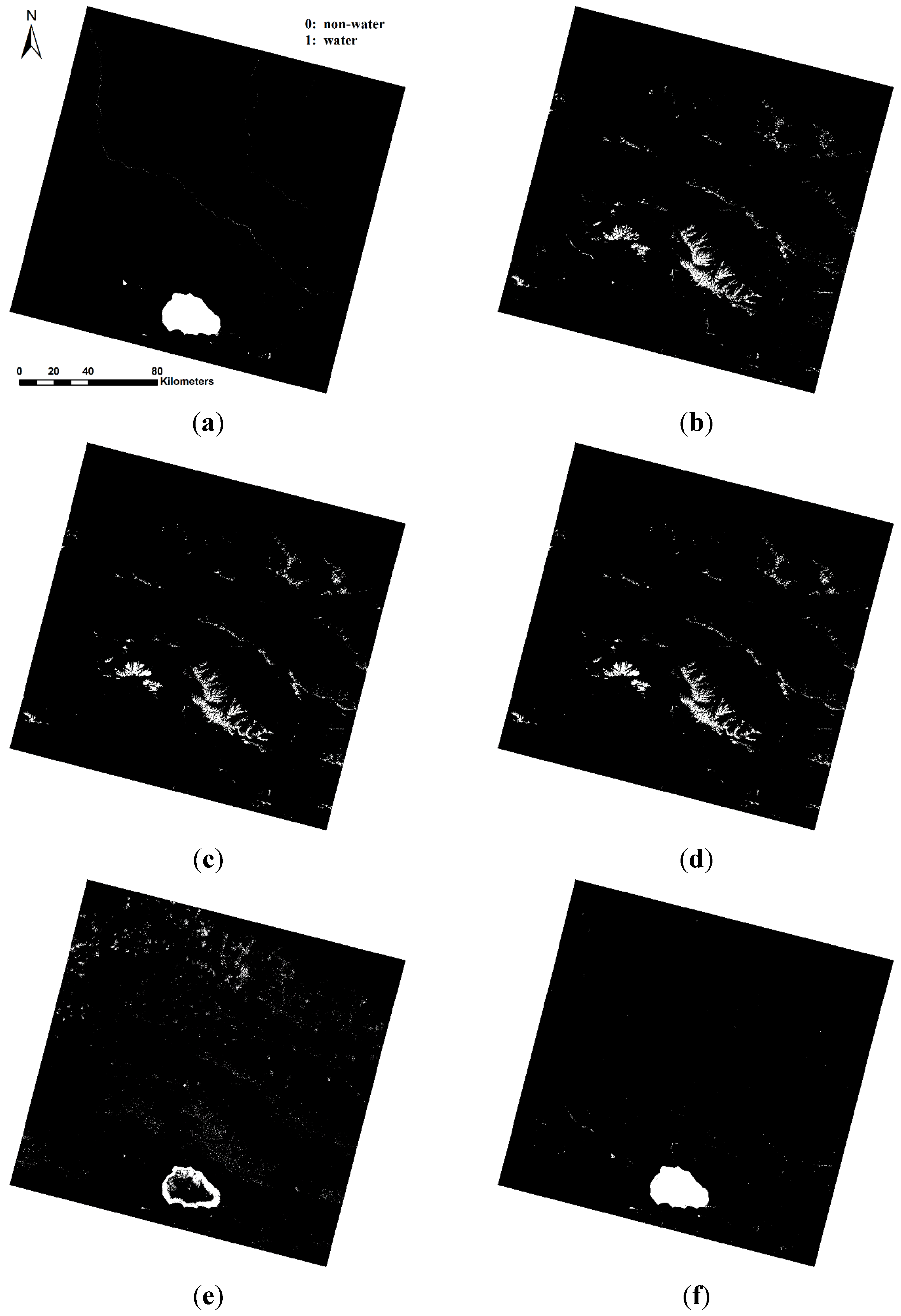
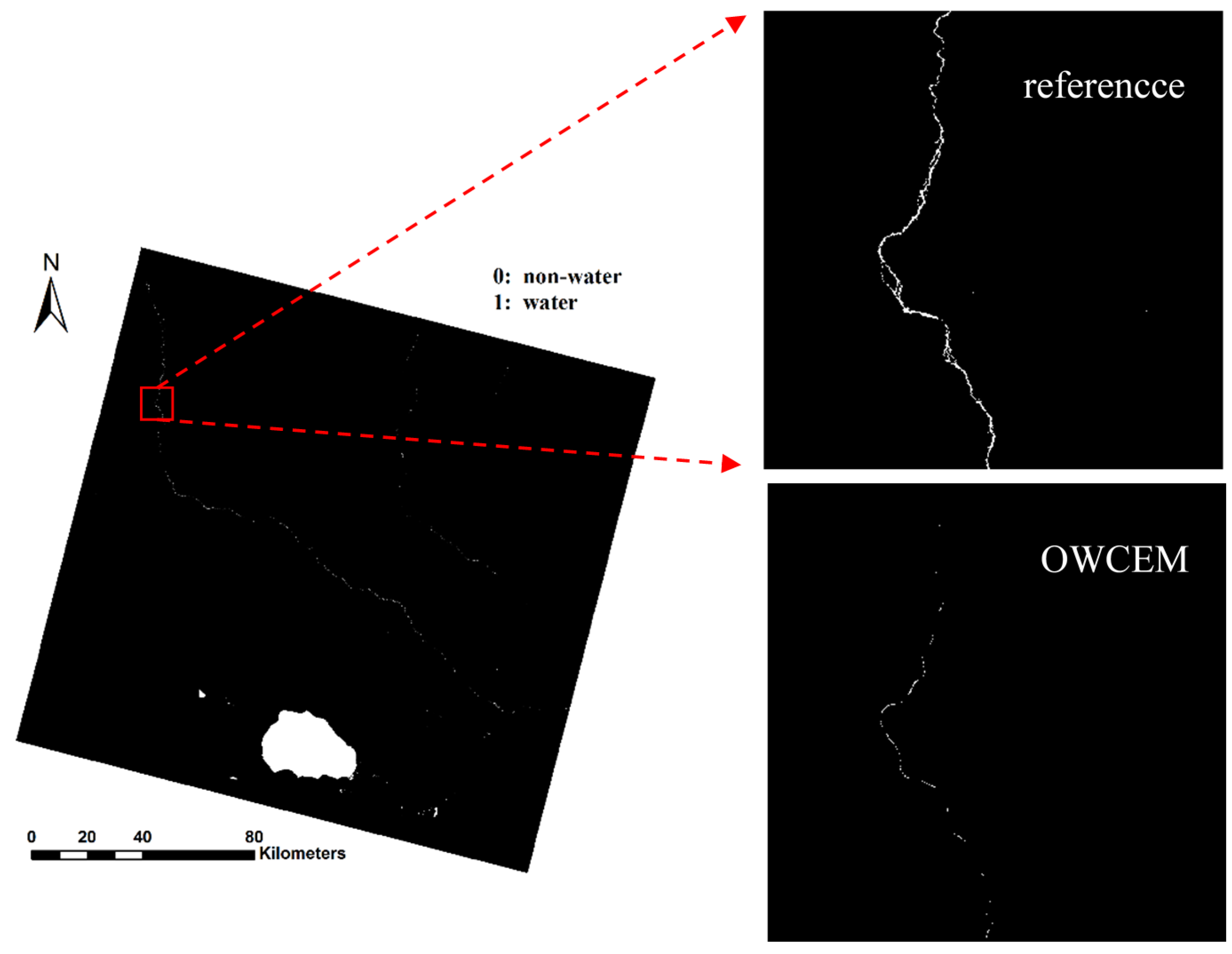
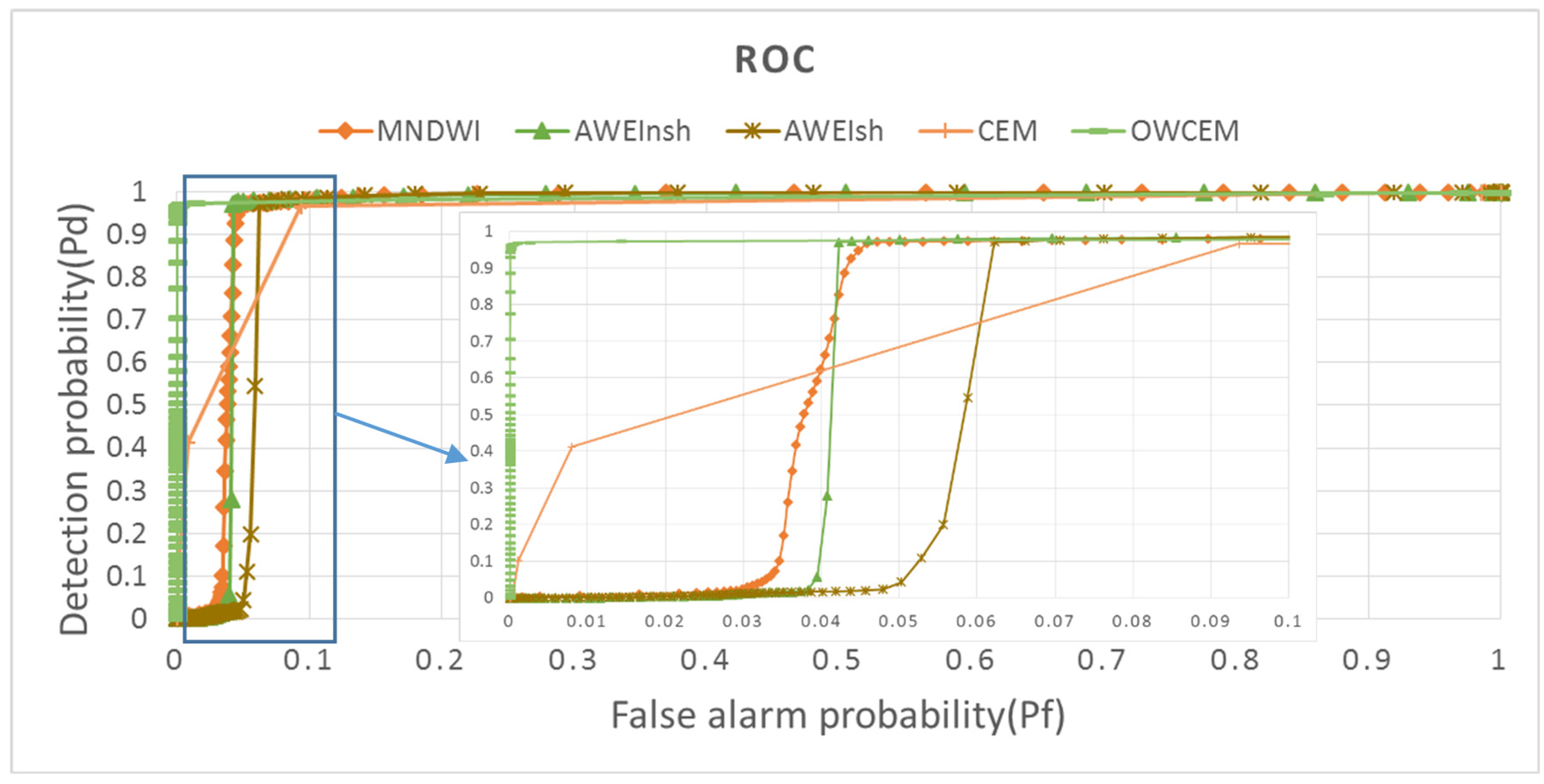
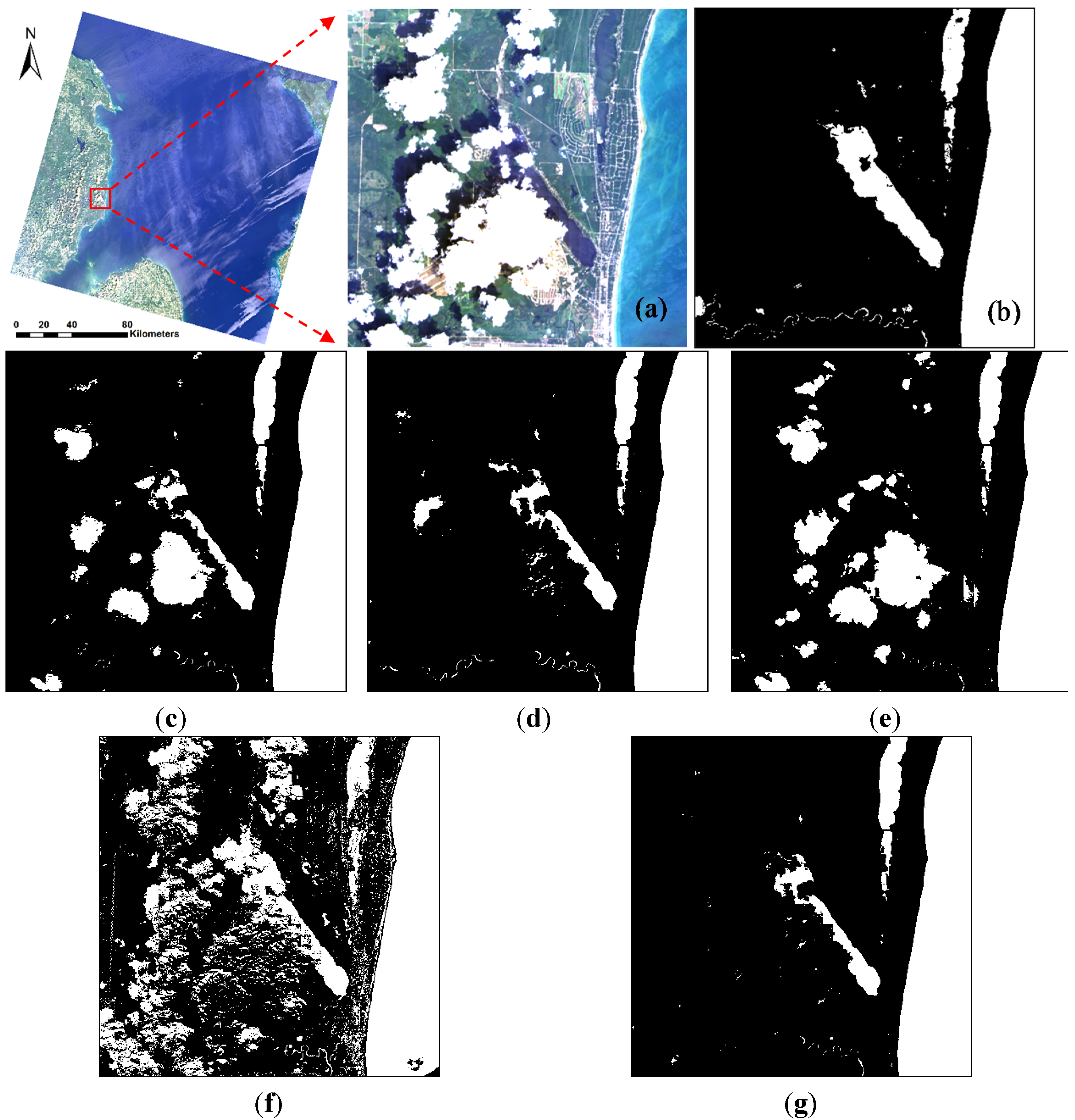
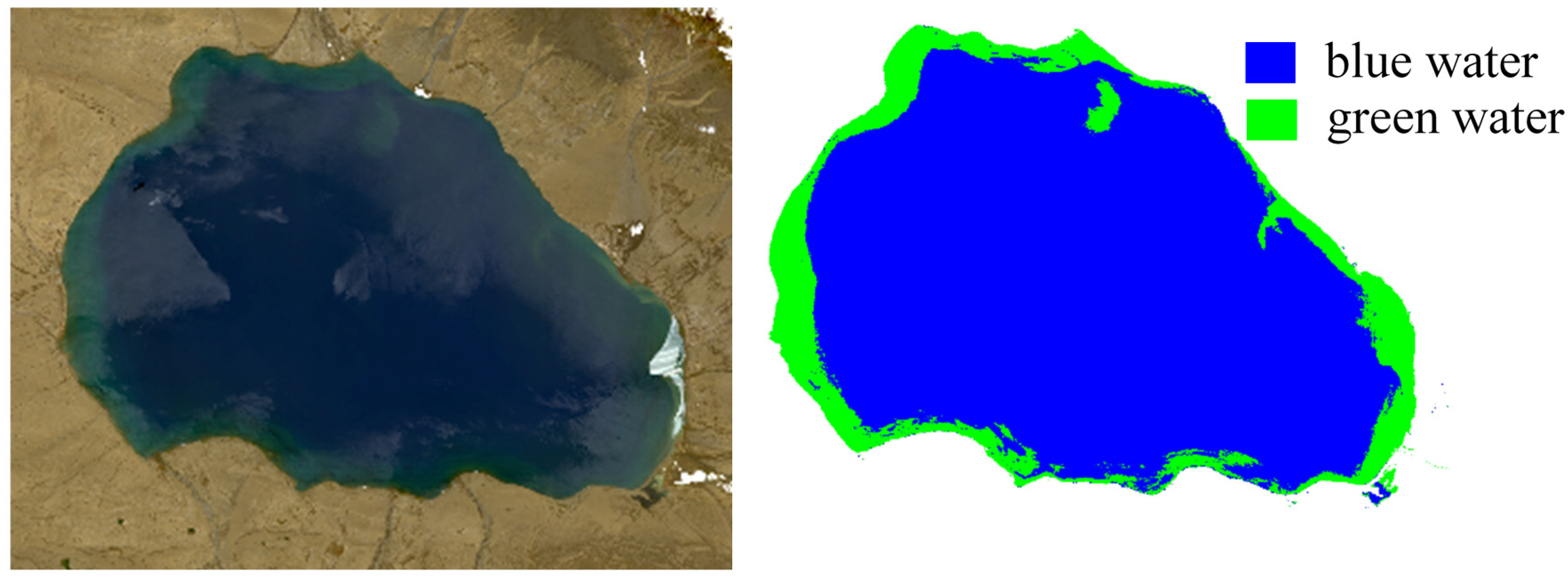
4.1. Hala Lake


| Classifier | MNDWI | AWEInsh | AWEIsh | CEM | OWCEM |
|---|---|---|---|---|---|
| Hala Lake | −0.0076 | −0.0152 | −0.0145 | 0.4744 | 0.9647 |
| Lake Huron | 0.9843 | 0.9843 | 0.9772 | 0.8473 | 0.9928 |

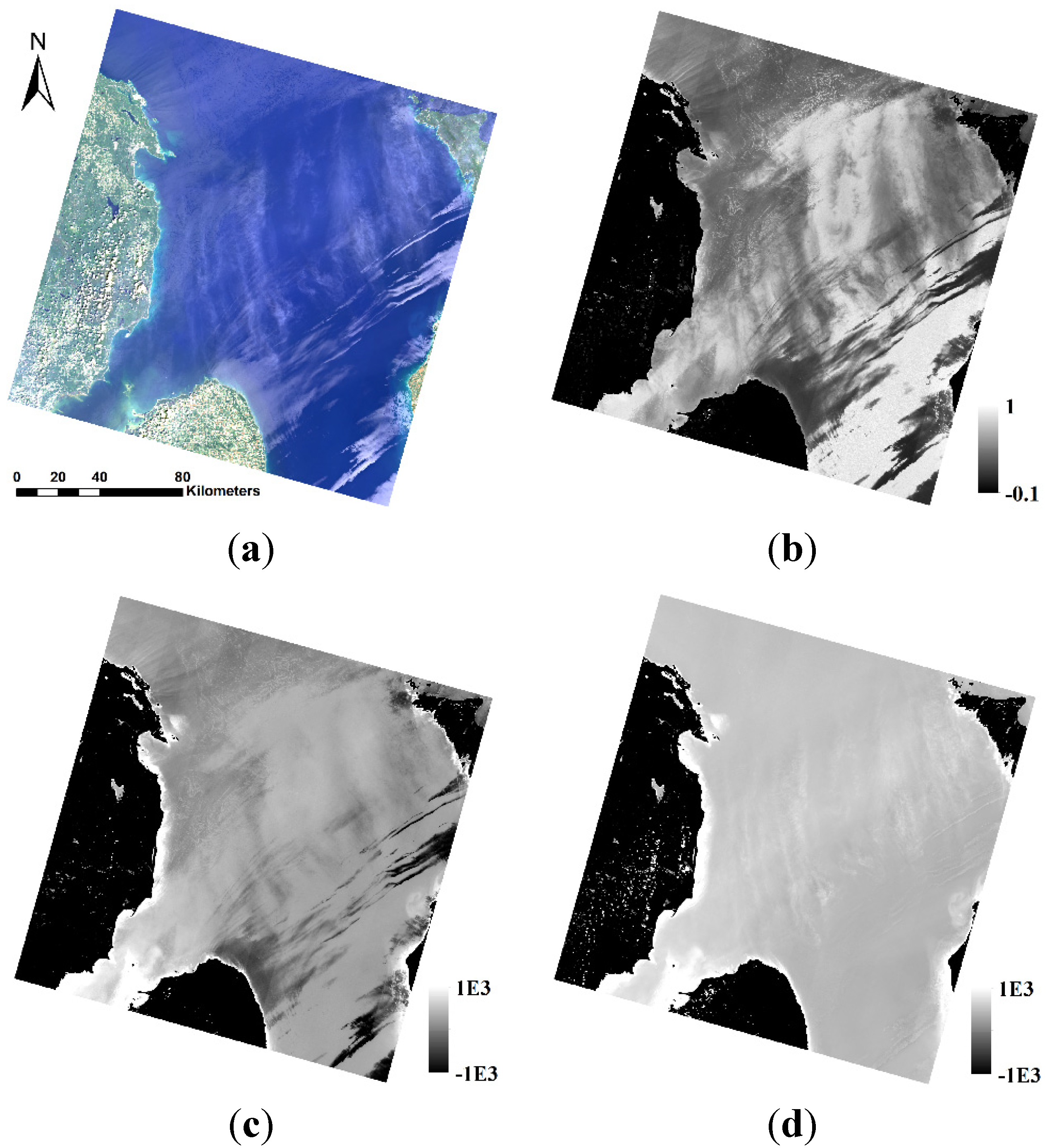
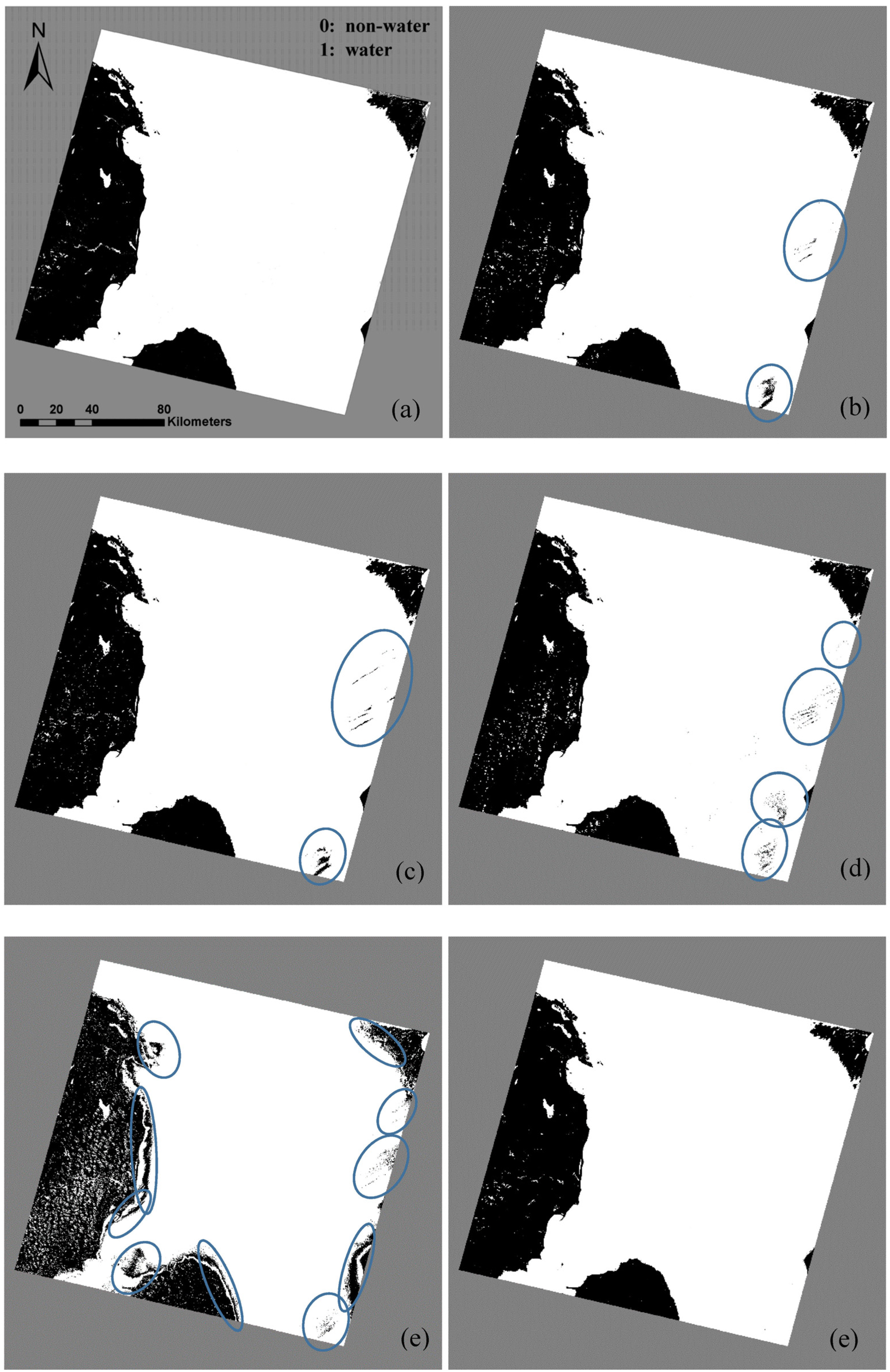
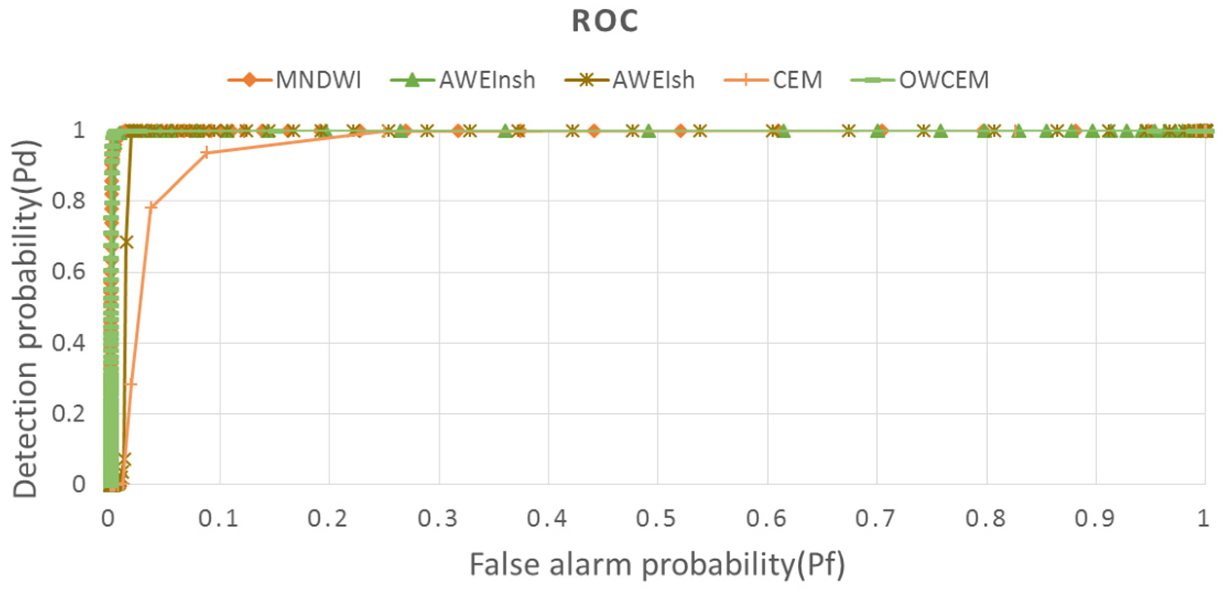
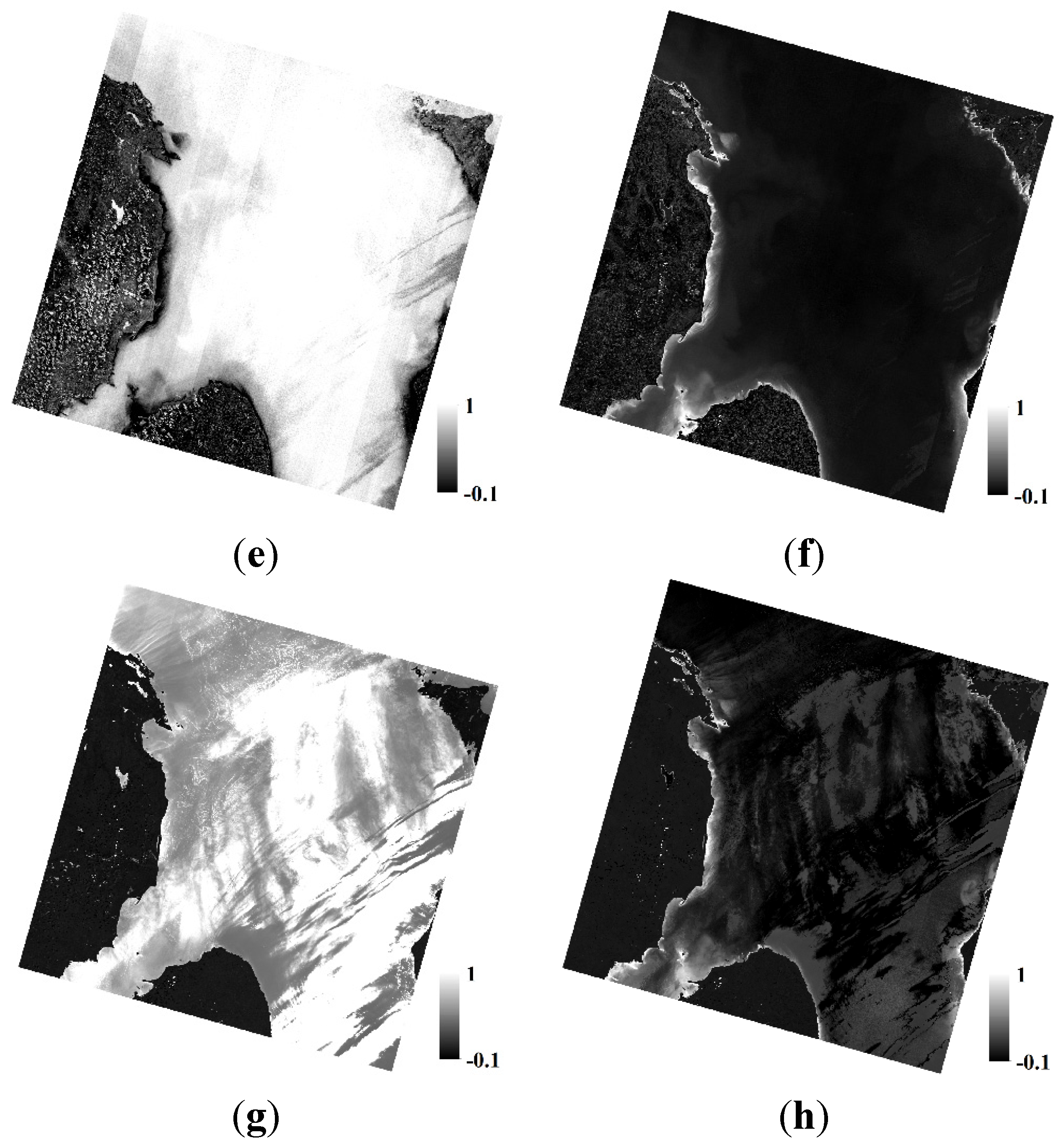
4.2. Lake Huron


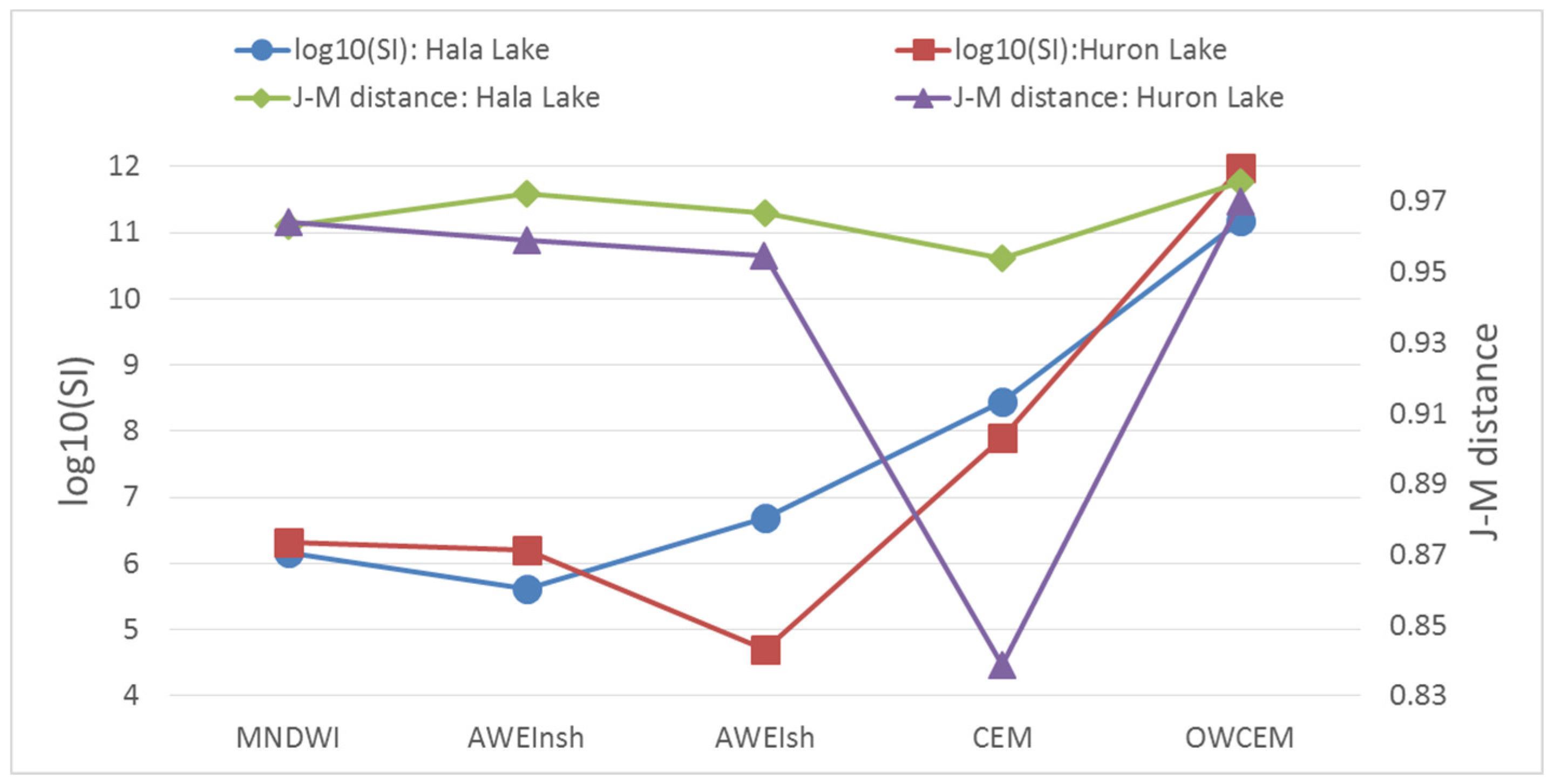
4.3. Analysis on Correlation between Channels
| Channel | MNDWI | MAWEInsh | MAWEIsh | corr | SAD | d | SID | n1 | MADWI + n2 | Corr + n2 |
|---|---|---|---|---|---|---|---|---|---|---|
| B1 | 0.8092 | 0.7894 | 0.6789 | 0.7224 | −0.7271 | 0.9281 | −0.5889 | −0.0003 | 0.8092 | 0.7224 |
| B2 | 0.8028 | 0.7821 | 0.6678 | 0.7107 | −0.7214 | 0.9365 | −0.5873 | −0.0003 | 0.8028 | 0.7107 |
| B3 | 0.7612 | 0.7349 | 0.6100 | 0.6526 | −0.6973 | 0.9624 | −0.5815 | −0.0003 | 0.7612 | 0.6526 |
| B4 | 0.7027 | 0.6726 | 0.5408 | 0.5797 | −0.6578 | 0.9755 | −0.5622 | −0.0003 | 0.7027 | 0.5797 |
| B5 | 0.5568 | 0.5293 | 0.3927 | 0.4341 | −0.5592 | 0.9773 | −0.4983 | −0.0002 | 0.5568 | 0.4341 |
| B6 | −0.4072 | −0.4587 | −0.4006 | −0.4457 | 0.0447 | 0.3687 | −0.1337 | −0.0001 | −0.4072 | −0.4457 |
| B7 | −0.3466 | −0.4085 | −0.3409 | −0.3981 | −0.0032 | 0.4068 | −0.1828 | −0.0001 | −0.3466 | −0.3981 |
| MNDWI | 1.0000 | 0.9934 | 0.9380 | 0.9135 | −0.8212 | 0.6131 | −0.6612 | −0.0002 | 1.0000 | 0.9135 |
| MAWEInsh | 0.9934 | 1.0000 | 0.9430 | 0.9179 | −0.7834 | 0.5758 | −0.6059 | −0.0002 | 0.9934 | 0.9179 |
| MAWEIsh | 0.9380 | 0.9430 | 1.0000 | 0.8907 | −0.7662 | 0.4877 | −0.6228 | −0.0003 | 0.9380 | 0.8907 |
| Corr | 0.9135 | 0.9179 | 0.8907 | 1.0000 | −0.7217 | 0.5031 | −0.5101 | −0.0002 | 0.9135 | 1.0000 |
| SAD | −0.8212 | −0.7834 | −0.7662 | −0.7217 | 1.0000 | −0.6286 | 0.9010 | 0.0002 | −0.8212 | −0.7217 |
| d | 0.6131 | 0.5758 | 0.4877 | 0.5031 | −0.6286 | 1.0000 | −0.5740 | −0.0003 | 0.6131 | 0.5031 |
| SID | −0.6612 | −0.6059 | −0.6228 | −0.5101 | 0.9010 | −0.5740 | 1.0000 | 0.0002 | −0.6612 | −0.5101 |
| Channel | MNDWI | MAWEInsh | MAWEIsh | Corr | SAD | d | SID | n1 | MNDWI + n2 | Corr + n2 |
|---|---|---|---|---|---|---|---|---|---|---|
| B1 | −0.1217 | −0.1842 | −0.1519 | −0.1056 | −0.0199 | 0.8368 | −0.0299 | −0.0001 | −0.1217 | −0.1056 |
| B2 | −0.1539 | −0.2128 | −0.1824 | −0.1368 | 0.0046 | 0.8543 | −0.0015 | −0.0001 | −0.1539 | −0.1368 |
| B3 | −0.3625 | −0.3824 | −0.3705 | −0.3655 | 0.2165 | 0.9321 | 0.2241 | 0.0001 | −0.3625 | −0.3655 |
| B4 | −0.3316 | −0.3677 | −0.3371 | −0.3445 | 0.1875 | 0.9282 | 0.1787 | 0.0000 | −0.3316 | −0.3445 |
| B5 | −0.8559 | −0.7331 | −0.7715 | −0.8981 | 0.8484 | 0.7830 | 0.8754 | 0.0004 | −0.8559 | −0.8981 |
| B6 | −0.7625 | −0.6909 | −0.6890 | −0.8210 | 0.7032 | 0.9015 | 0.7106 | 0.0004 | −0.7624 | −0.8210 |
| B7 | −0.6181 | −0.5957 | −0.5680 | −0.6761 | 0.5204 | 0.9464 | 0.5097 | 0.0002 | −0.6181 | −0.6761 |
| MNDWI | 1.0000 | 0.9547 | 0.9690 | 0.8948 | −0.8303 | −0.5075 | −0.8658 | −0.0005 | 1.0000 | 0.8948 |
| MAWEInsh | 0.9547 | 1.0000 | 0.9851 | 0.7579 | −0.6469 | −0.4524 | −0.6802 | −0.0004 | 0.9547 | 0.7579 |
| MAWEIsh | 0.9690 | 0.9851 | 1.0000 | 0.7743 | −0.6782 | −0.4427 | −0.7359 | −0.0005 | 0.9690 | 0.7743 |
| Corr | 0.8948 | 0.7579 | 0.7743 | 1.0000 | −0.9578 | −0.5923 | −0.9322 | −0.0005 | 0.8948 | 1.0000 |
| SAD | −0.8303 | −0.6469 | −0.6782 | −0.9578 | 1.0000 | 0.4879 | 0.9730 | 0.0005 | −0.8303 | −0.9578 |
| d | −0.5075 | −0.4524 | −0.4427 | −0.5923 | 0.4879 | 1.0000 | 0.4676 | 0.0002 | −0.5075 | −0.5923 |
| SID | −0.8658 | −0.6802 | −0.7359 | −0.9322 | 0.9730 | 0.4676 | 1.0000 | 0.0005 | −0.8658 | −0.9322 |
| Data used for OWCEM | Hala Lake | Lake Huron |
|---|---|---|
| 7 Landsat bands, MNDWI | 0.8024 | 0.9428 |
| 7 Landsat bands, MNDWI, n1 | 0.8024 | 0.9428 |
| 7 Landsat bands, MNDWI, MNDWI + n2 | 0.8022 | 0.9427 |
| 7 Landsat bands, MNDWI, MAWEIsh | 0.9638 | 0.9761 |
| 7 Landsat bands, MNDWI, MAWEIsh, d | 0.9640 | 0.9916 |
| 7 Landsat bands, corr | 0.5505 | 0.9907 |
| 7 Landsat bands, corr, n1 | 0.5500 | 0.9907 |
| 7 Landsat bands, corr, corr + n2 | 0.5501 | 0.9907 |
| 7 Landsat bands, corr, SAD | 0.9263 | 0.9927 |
5. Discussion and Perspectives
6. Conclusions
Acknowledgments
Author Contributions
Conflicts of Interest
References
- Roberts, N.; Taieb, M.; Barker, P.; Damnati, B.; Icole, M.; Williamson, D. Timing of the younger dryas event in east africa from lake-level changes. Nature 1993, 366, 146–148. [Google Scholar] [CrossRef]
- Gong, P. Remote sensing of environmental change over china: A review. Chin. Sci. Bull. 2012, 57, 2793–2801. [Google Scholar] [CrossRef]
- Feyisa, G.L.; Meilby, H.; Fensholt, R.; Proud, S.R. Automated water extraction index: A new technique for surface water mapping using landsat imagery. Remote Sens. Environ. 2014, 140, 23–35. [Google Scholar] [CrossRef]
- Sun, F.; Zhao, Y.; Gong, P.; Ma, R.; Dai, Y. Monitoring dynamic changes of global land cover types: Fluctuations of major lakes in china every 8 days during 2000–2010. Chin. Sci. Bull. 2014, 59, 171–189. [Google Scholar] [CrossRef]
- McIver, D.K.; Friedl, M.A. Using prior probabilities in decision-tree classification of remotely sensed data. Remote Sens. Environ. 2002, 81, 253–261. [Google Scholar] [CrossRef]
- Tulbure, M.G.; Broich, M. Spatiotemporal dynamic of surface water bodies using landsat time-series data from 1999 to 2011. ISPRS J. Photogramm. Remote Sens. 2013, 79, 44–52. [Google Scholar] [CrossRef]
- Sivanpillai, R.; Miller, S.N. Improvements in mapping water bodies using aster data. Ecol. Inform. 2010, 5, 73–78. [Google Scholar] [CrossRef]
- Sethre, P.R.; Rundquist, B.C.; Todhunter, P.E. Remote detection of prairie pothole ponds in the devils lake basin, north dakota. GISci. Remote Sens. 2005, 42, 277–296. [Google Scholar] [CrossRef]
- Work, E.A., Jr.; Gilmer, D.S. Utilization of satellite data for inventorying prairie ponds and lakes. Photogramm. Eng. Remote Sens. 1976, 42, 685–694. [Google Scholar]
- Rundquist, D.C.; Lawson, M.P.; Queen, L.P.; Cerveny, R.S. The relationship between summer-season rainfall events and lake-surface area. J. Am. Water Resour. Assoc. 1987, 23, 493–508. [Google Scholar] [CrossRef]
- McFeeters, S.K. The use of the normalized difference water index (NDWI) in the delineation of open water features. Int. J. Remote Sens. 1996, 17, 1425–1432. [Google Scholar] [CrossRef]
- Xu, H. Modification of normalised difference water index (NDWI) to enhance open water features in remotely sensed imagery. Int. J. Remote Sens. 2006, 27, 3025–3033. [Google Scholar] [CrossRef]
- Boland, D.H. Trophic Classification of Lakes Using Landsat-1 (erts-1) Multispectral Scanner Data; U.S. Environmental Protection Agency: Corvallis, OR, USA, 1976; p. 265.
- Ji, L.; Zhang, L.; Wylie, B. Analysis of dynamic thresholds for the normalized difference water index. Photogramm. Eng. Remote Sens. 2009, 75, 1307–1317. [Google Scholar] [CrossRef]
- Rogers, A.S.; Kearney, M.S. Reducing signature variability in unmixing coastal marsh thematic mapper scenes using spectral indices. Int. J. Remote Sens. 2004, 25, 2317–2335. [Google Scholar] [CrossRef]
- Duan, Z.; Bastiaanssen, W.G.M. Estimating water volume variations in lakes and reservoirs from four operational satellite altimetry databases and satellite imagery data. Remote Sens. Environ. 2013, 134, 403–416. [Google Scholar] [CrossRef]
- Poulin, B.; Davranche, A.; Lefebvre, G. Ecological assessment of phragmites australis wetlands using multi-season spot-5 scenes. Remote Sens. Environ. 2010, 114, 1602–1609. [Google Scholar] [CrossRef]
- Hui, F.; Xu, B.; Huang, H.; Yu, Q.; Gong, P. Modelling spatial-temporal change of poyang lake using multitemporal landsat imagery. Int. J. Remote Sens. 2008, 29, 5767–5784. [Google Scholar] [CrossRef]
- Chang, C.-I.; Althouse, M.L.G.; Sun, T.-L. Unsupervised interference rejection approach to target detection and classification for hyperspectral imagery. Opt. Eng. 1998, 37, 735–743. [Google Scholar] [CrossRef]
- Farrand, W.H.; Harsanyi, J.C. Mapping the distribution of mine tailings in the coeur d’alene river valley, idaho, through the use of a constrained energy minimization technique. Remote Sens. Environ. 1997, 59, 64–76. [Google Scholar] [CrossRef]
- Manolakis, D.; Shaw, G. Detection algorithms for hyperspectral imaging applications. IEEE Signal Proc. Mag. 2002, 19, 29–43. [Google Scholar] [CrossRef]
- Harsanyi, J.C. Detection and Classification of Subpixel Spectral Signatures in Hyperspectral Image Sequences; University of Maryland: College Park, MD, USA, 1993. [Google Scholar]
- Du, Q.; Ren, H.; Chang, C.-I. A comparative study for orthogonal subspace projection and constrained energy minimization. IEEE Trans. Geosci. Remote Sens. 2003, 41, 1525–1529. [Google Scholar] [CrossRef]
- Arora, M.K.; Bansal, S.; Khare, S.; Chauhan, K. Comparative assessment of some target detection algorithms for hyperspectral images. Def. Sci. J. 2013, 63, 53–62. [Google Scholar] [CrossRef]
- Manolakis, D.; Shaw, G.; Keshava, N. Comparative analysis of hyperspectral adaptive matched filter detector. Proc. SPIE 2000. [Google Scholar] [CrossRef]
- Chen, J.Y.; Reed, I.S. A detection algorithm for optical targets in clutter. IEEE Trans. Aerosp. Electron. Syst. 1987, AES-23, 46–59. [Google Scholar] [CrossRef]
- Manolakis, D.; Lockwood, R.; Cooleyb, T.; Jacobson, J. Is there a best hyperspectral detection algorithm? Proc. SPIE 2009. [Google Scholar] [CrossRef]
- Manolakis, D.; Lockwood, R.; Cooleyb, T.; Jacobson, J. Hyperspectral detection algorithms: Use covariances or subspaces? Proc. SPIE 2009. [Google Scholar] [CrossRef]
- DiPietro, R.S.; Manolakis, D.; Lockwood, R.; Cooleyb, T.; Jacobson, J. Performance evaluation of hyperspectral detection algorithms for sub-pixel objects. Proc. SPIE 2010. [Google Scholar] [CrossRef]
- Manolakis, D.; Marden, D.; Kerekes, J.; Shaw, G. On the statistics of hyperspectral imaging data. Proc. SPIE 2001. [Google Scholar] [CrossRef]
- Funk, C.C.; Theiler, J.; Roberts, D.A.; Borel, C.C. Clustering to improve matched filter detection of weak gas plumes in hyperspectral thermal imagery. IEEE Trans. Geosci. Remote Sens. 2001, 39, 1410–1420. [Google Scholar] [CrossRef]
- Minet, J.; Taboury, J.; Goudail, F.; Péalat, M.; Roux, N.; Lonnoy, J.; Ferrec, Y. Influence of band selection and target estimation error on the performance of the matched filter in hyperspectral imaging. Appl. Opt. 2011, 50, 4276–4284. [Google Scholar] [CrossRef] [PubMed]
- Ren, H.; Wang, C.-M.; Chang, C.-I.; Liu, J.-M.; Yang, C.-W.; Ma, D.-J.; Chieu, B.-C.; Lo, C.-S.; Chung, P.-C. Generalized constrained energy minimization approach to subpixel target detection for multispectral imagery. Opt. Eng. 2000, 39, 1275–1281. [Google Scholar] [CrossRef]
- Geng, X.; Ji, L.; Sun, K.; Zhao, Y. CEM: More bands, better performance. IEEE Geosci. Remote Sens. Lett. 2014, 11, 1–5. [Google Scholar] [CrossRef]
- Geng, X.; Zhao, Y. Principle of small target detection for hyperspectral imagery. Sci. China Earth Sci. 2007, 50, 1225–1231. [Google Scholar] [CrossRef]
- Wünnemann, B.; Wagner, J.; Zhang, Y.; Yan, D.; Wang, R.; Shen, Y.; Fang, X.; Zhang, J. Implications of diverse sedimentation patterns in hala lake, qinghai province, china for reconstructing late quaternary climate. J. Paleolimnol. 2012, 48, 725–749. [Google Scholar] [CrossRef]
- Gong, P.; Wang, J.; Yu, L.; Zhao, Y.; Zhao, Y.; Liang, L.; Niu, Z.; Huang, X.; Fu, H.; Liu, S.; et al. Finer resolution observation and monitoring of global land cover: First mapping results with landsat tm and etm+ data. Int. J. Remote Sens. 2012, 34, 2607–2654. [Google Scholar] [CrossRef]
- Chang, C.-I. An information-theoretic approach to spectral variability, similarity, and discrimination for hyperspectral image analysis. IEEE Trans. Inf. Theory 2000, 46, 1927–1932. [Google Scholar] [CrossRef]
- Sun, F.; Sun, W.; Chen, J.; Gong, P. Comparison and improvement of methods for identifying waterbodies in remotely sensed imagery. Int. J. Remote Sens. 2012, 33, 6854–6875. [Google Scholar] [CrossRef]
- Geng, X.; Xiao, Z.; Ji, L.; Zhao, Y.; Wang, F. A gaussian elimination based fast endmember extraction algorithm for hyperspectral imagery. ISPRS J. Photogramm. Remote Sens. 2013, 79, 211–218. [Google Scholar] [CrossRef]
- Ji, L.; Geng, X.; Yu, K.; Zhao, Y. A new non-negative matrix factorization method based on barycentric coordinates for endmember extraction in hyperspectral remote sensing. Int. J. Remote Sens. 2013, 34, 6577–6586. [Google Scholar] [CrossRef]
- Acito, N.; Resta, S.; Diani, M.; Corsini, G. Robust technique for anomalous change detection in airborne hyperspectral imagery based on automatic and adaptive band selection. Opt. Eng. 2013, 52. [Google Scholar] [CrossRef]
© 2015 by the authors; licensee MDPI, Basel, Switzerland. This article is an open access article distributed under the terms and conditions of the Creative Commons Attribution license (http://creativecommons.org/licenses/by/4.0/).
Share and Cite
Ji, L.; Geng, X.; Sun, K.; Zhao, Y.; Gong, P. Target Detection Method for Water Mapping Using Landsat 8 OLI/TIRS Imagery. Water 2015, 7, 794-817. https://doi.org/10.3390/w7020794
Ji L, Geng X, Sun K, Zhao Y, Gong P. Target Detection Method for Water Mapping Using Landsat 8 OLI/TIRS Imagery. Water. 2015; 7(2):794-817. https://doi.org/10.3390/w7020794
Chicago/Turabian StyleJi, Luyan, Xiurui Geng, Kang Sun, Yongchao Zhao, and Peng Gong. 2015. "Target Detection Method for Water Mapping Using Landsat 8 OLI/TIRS Imagery" Water 7, no. 2: 794-817. https://doi.org/10.3390/w7020794
APA StyleJi, L., Geng, X., Sun, K., Zhao, Y., & Gong, P. (2015). Target Detection Method for Water Mapping Using Landsat 8 OLI/TIRS Imagery. Water, 7(2), 794-817. https://doi.org/10.3390/w7020794