
Spatial and Temporal Streamflow Trends in Northern Taiwan


1
Department of Resources Engineering, National Cheng Kung University, Tainan 70101, Taiwan
2
Three Gorges Research Center for Geo-hazard, China University of Geosciences, Wuhan 430074, China
*
Author to whom correspondence should be addressed.
Water 2015, 7(2), 634-651; https://doi.org/10.3390/w7020634
Submission received: 24 November 2014
/
Revised: 9 January 2015
/
Accepted: 27 January 2015
/
Published: 10 February 2015
Abstract
:Streamflow is an important factor in the study of water resource management, floods, and droughts. Dramatic climate change has created extreme rainfall distributions, making the study of streamflow trends and variability even more crucial. In this study, the long-term streamflow data and trends recorded at gauging stations in Northern Taiwan are analyzed using the Mann-Kendall test. The data used for trend analysis are the average annual streamflow, the average seasonal streamflow, and the high and low flows. The slope trend is calculated using the Theil-Sen estimator. Finally, change point analysis is conducted using the Mann-Whitney-Pettit test and the cumulative deviation test to gain further information about the change points and to understand the changes in streamflow before and after the change points. The average annual streamflow of the 12 gauging stations in the study area is analyzed using the Mann-Kendall test. The results show that of the 12 gauging stations, only the Ximen Bridge Station in the Lanyang River basin show a significant downward streamflow trend. Results of the monthly and seasonal average streamflow analysis show that in the spring, 72.2% of the gauging stations showed upward streamflow trends, most of which were located in the Tamsui River and the Touqian River basins. The high and low flow data analysis shows that the Ximen Bridge Station was the only gauging station to feature a significant downward streamflow trend for both high and low flows. This distribution pattern provides valuable information for regional hydrological studies and water management.
1. Introduction
Due to global warming, the global climate has experienced drastic changes such as the rise in global temperature, the increase in melting ice in the Alps and the North and South Poles, and uneven rainfall distribution [1]. These changes have had a significant impact on hydrological factors, such as streamflows, base flows, and groundwater levels. Investigations on hydrological factor trends have thus become increasingly crucial [2,3,4]. Located at the boundary between the Philippine Sea Plate and the Eurasian Plate, Taiwan features violent plate activity and a rapid rise in terrain altitude. For example, the Western regions contain plains that average 100 m in elevation while the Central and Eastern mountain range have mountains that average 3000 m in elevation. Because of the rapid rise in terrain altitude, streams in Taiwan are short and turbulent. Streamflow is an important factor in studies of water resource management, floods, and droughts. In addition, dramatic climate change has created extreme rainfall distributions, making the study of streamflow trends and variability even more crucial.
The Mann-Kendall test has been widely used in streamflow trend analysis. Concerning research on mainland-based climate zones, Lins and Slack [5] analyzed data from 395 U.S. gauging stations in climate-sensitive regions using the Mann-Kendall test, with results showing general upward streamflow trends; only a few Northwestern and Southeastern regions exhibited downward streamflow trends. The results showed that the climate in the U.S. is humid but has not reached extreme humidity. Zhang et al. [6] investigated 30–50 years of streamflow data collected from 11 Canadian gauging stations, with results showing that during this period, the average monthly streamflow frequently decreased, and the average annual streamflow decreased for southern cities. Kahya and Kalayci [7] analyzed the monthly streamflow data for 26 Turkish basins over the past 31 years, with results showing downward streamflow trends, which could be attributed to a drop in rainfall and a rise in temperature. Chen et al. [8] selected the Kaidu River basin, located in the Northwestern Arid Region of China, as the study area and conducted an analysis using annual streamflow data from 1960 to 2009. They then conducted trend and change point analyses using the Mann-Kendall test and the Mann-Kendall-Sneyers test, respectively. The results of their analyses revealed that the Kaidu River basin showed a significant annual streamflow increase and that the change point occurred in 1993. They subsequently divided the time periods into 1960–1993 and 1994–2009, where the former was defined as a “natural period” and the latter as a “human-induced period.”
Regarding research conducted on island-based climate zones, Dixon et al. [9] analyzed the seasonal and annual data collected from 56 West England gauging stations. The data time period spanned 40 years (from 1962 to 2001). The study results showed significant upward streamflow trends for both high and low flows, whereas the average streamflow remained relatively stable. Dixon et al. [9] subsequently divided the streams into East and West, where the Western mountainous region showed significant upward streamflow trends, particularly in high flow during the fall and winter. Baggaley et al. [10] investigated the 1929–2004 streamflow records of the Dee River in Northeast Scotland and found that when investigating the streamflow and rainfall spatio-temporal correlation changes, one must also consider factors that contribute to snowfall changes in the alpine catchment area. This is because snowfall is highly correlated to downward rainfall trends. Their study also found that to highlight the peak streamflow in a correlation system, the use of hours as the unit of measurement is superior to the use of days. Hannaford et al. [11] analyzed the 1969–2008 data of 89 U.K. catchment areas, with the study results showing that seasonal data analyses are prone to the influence of irregular runoff increases, high flow in the winter and fall, and low flow in the spring. Observations made of the lowlands in Southeast England revealed the presence of spatial heterogeneity in trends. Therefore, when increasing the scale of the basin in a study area, one must carefully consider the issue of spatial heterogeneity. Bassiouni and Oki [12] analyzed the 1913–2008 streamflow data for Hawaii using the Mann-Kendall test, with results showing that both the high and maximum flow trends exhibited significant decreases.
The Mann-Kendall test is primarily used to determine whether a series of numbers demonstrate a significant trend. However, it cannot be used to calculate the extent of the upward or downward trend. Therefore, a trend slope calculation method is normally used in conjunction with the Mann-Kendall test. The Theil-Sen estimator is a commonly used trend slope calculation method, particularly in a hydrological factor trend analysis. In such an analysis, it is used together with other trend analysis methods to perform quantitative analyses on trend significance [11,12,13,14,15]. Thus, in this study, the Theil-Sen estimator is used to calculate the trend slopes to obtain the extent of trend changes.
When performing long-term trend analyses on hydrological factors, the trends obtained signify the overall characteristics of the hydrological factors. However, world climate change has created dissimilar hydrology trends at different time periods. The intersection where two dissimilar trends meet is called a change point. To determine whether change points exist in the long-term data in this study, the Mann-Whitney-Pettit test and the cumulative deviation test, two tests commonly used in hydrology analyses, are used [14,16,17,18].
As mentioned, the Mann-Kendall trend test is widely used in the spatio-temporal analyses of streamflow sequences for various climate regions. Thus, streamflow trends were analyzed in this study. As a densely populated area, the northern regions of Taiwan have a high demand for water. However, climate change over recent years has created climate anomalies, resulting in severe water shortages during the originally rainy winter and spring seasons [19]. To reduce the impact of climate change on water use in the northern regions of Taiwan, the hydrology information of the regions must be fully understood and effectively managed. To explore the streamflow changes in the northern regions of Taiwan, the long-term streamflow data of 12 gauging stations in the regions are selected. The average annual streamflow, average monthly streamflow, and high and low flows are analyzed using the Mann-Kendall test, and significant trends and distribution changes are discussed. The trend slope is calculated using the Theil-Sen estimator, which produces the amount of change in trends. Finally, the change points in the long-term streamflow data are identified using the Mann-Whitney-Pettit test and the cumulative deviation test, and the changes in streamflow before and after the change points are explored. These research methods are used to determine long-term streamflow trend changes in the northern regions of Taiwan and the trend change spatial variability.
2. Study Methods
2.1. Mann-Kendall Test
The Mann-Kendall test [20,21] is a nonparametric test method that can be used to verify whether trends are significant by measuring the magnitude of the relationship between successive data points. Its advantages include the ability to process missing data and extrema in a number series. The formula is described below.
Assuming a time series t1, t2, …, tn feature corresponding to the data series x1, x2, …, xn, the statistical value S of the Mann-Kendall test is:
When n ≥ 10, the statistical value S of the Mann-Kendall test is similar to a normal distribution, with a mean of 0. The variance is:
The Z value can be used to determine whether the time series data exhibits a significant trend. The Z value is defined as:
|Z| > Z(α/2) signifies that the time series data show a significant trend. A positive (negative) S value means a significant upward (downward) trend. α is the significance level. Because varying α correspond to varying Z(α/2), the method suggests that the definition of significant trends in statistics changes. In this study, the significance level is set at 0.05, making Z(α/2) = 1.96. Therefore, when the time series data produces |Z| > 1.96, there is a significant upward or downward trend.
2.2. Theil-Sen Estimator
In this study, the Theil-Sen estimator is used to calculate the trend slopes. The Theil-Sen estimator was introduced by Sen in 1968 [22] to calculate true trend slopes. In the study, Sen indicated that when a time series exhibits linear trend characteristics, the true slope can be calculated using simple equations. One of the advantages of the Theil-Sen estimator is that it is not prone to the influence of extreme values. In general, when a time series contains extreme values, linear regression methods are prone to their influence, resulting in overestimated and underestimated slopes. In contrast, because the Theil-Sen estimator takes the median of a slope between two points in a time series as the true slope, it is unaffected by extreme values. The time series true slope calculation formula is:
where β is the slope between two data points in the time series and xj and xk are the corresponding data values for time points j and k (j > k), respectively. After the trend slopes have been calculated, the original data series are used to derive the trend slope equation:
where Yt is the data value obtained from the trend slope equation, t is the time, and Xt is the intercept.
After the trend slope has been obtained, the changes in the average annual streamflow, average monthly streamflow, and high and low streamflow are calculated by employing the equation used by Petrow and Merz [23] to determine the amount of change in the data series:
where is the amount of change observed in the data series, is the last piece of the trend slope data, and is the first piece of the trend slope data.
2.3. Mann-Whitney-Pettit Test
The Mann-Whitney-Pettit test [24] is primarily used to assess significant change points that exist in a number series. By definition, when change point exists in a number series , . Therefore, when change points do not exist in a number series, will continue to rise and no turning points will be observed. However, when change points do exist in a number series, will decrease and create turning points. When a number series shows multiple turning points, the number of change points in the number series may potentially be more than one. The change point equation is:
To determine whether change points exist, the in Equation (8), which is the extreme value of , may be used. Equation (9) is used to calculate the probability (P) of the said change points. In this study, P = 0.9 was set as the test standard; that is, a point in a number series was considered as a change point when P > 0.9.
For some number series, multiple change points may be identified. When this occurs, the following equation may be used to calculate the annual value. The intervals for the annual values that exceed the test standard can then be derived.
2.4. Cumulative Deviation Test
The cumulative deviation test [25] is primarily used to determine whether a number series is uniform. The test involves calculating the difference () between each data value () and the mean of the number series (). If the number series is uniform, will oscillate at 0. The equation is:
where n is the number of data values. After has been calculated, the standard deviation () is used to correct to produce an number series. Next, the maximum value in the number series is identified, which is used to calculate the statistical test value .
If is greater than the critical value, the number series is not uniform. The critical value varies with the number of years of the data record, as shown in Table 1.

Table 1.
Percentage points of [25].
| n | |||
|---|---|---|---|
| 90% | 95% | 99% | |
| 10 | 1.05 | 1.14 | 1.29 |
| 20 | 1.10 | 1.22 | 1.42 |
| 30 | 1.12 | 1.24 | 1.46 |
| 40 | 1.13 | 1.26 | 1.50 |
| 50 | 1.14 | 1.27 | 1.52 |
| 100 | 1.17 | 1.29 | 1.55 |
| 1.22 | 1.36 | 1.63 | |
3. Study Area
In this study, the northern water resource regions listed by the Water Resources Agency of the Ministry of Economic Affairs were selected as the study area. These regions include the following administrative areas: Yilan County, Keelung City, New Taipei City, Taipei City, Taoyuan County, and Hsinchu County. The regions contain five terrain types, namely, plains, hills, highlands, basins, and mountains. Regions featuring plains primarily comprise the Taoyuan Alluvial Fan, the Hsinchu Plains, and the Eastern Yilan Delta; regions containing hills consist of the Keelung Hills and the Zhudong Hills; regions with highlands include the Linkou Plateau; regions with basins include the Taipei Basin; and regions featuring mountains primarily comprise the northernmost Tatun Mountains and the Central Backbone Range. These regions embody a variety of terrain characteristics; terrains ranging from those less than 100 m in elevation (plains), to less than 500 m in elevation (hills), and to more than 1000 m in elevation (mountains).
Rainfall in the northern regions of Taiwan during the summer and winter seasons primarily comes from typhoons and northeast monsoons, respectively. The Northern Taiwan regions receive rainfall all year long. For example, the Yilan region can have up to 350 days of rainfall. The average annual rainfall in the northern regions of Taiwan is 2937 mm, which is higher than that in Central, Southern, and Eastern Taiwan.
The main rivers in the Northern Taiwan regions are the Tamsui River, the Lanyang River, the Fengshan River, and the Touqian River, which have drainage basin areas of 2726, 978, 250.1, and 565.9 km2, respectively. The historical overall average annual streamflow is approximately 15.1 × 10⁹ m3, which is lower than those of the central, southern, and eastern regions. Historical data show a significant difference in the Northern Taiwan region streamflow between the dry and wet seasons, where the overall streamflows are approximately 5.62 × 10⁹ and 9.48 × 10⁹ m3 during the dry (November to April) and wet (May to October) seasons, respectively [19].
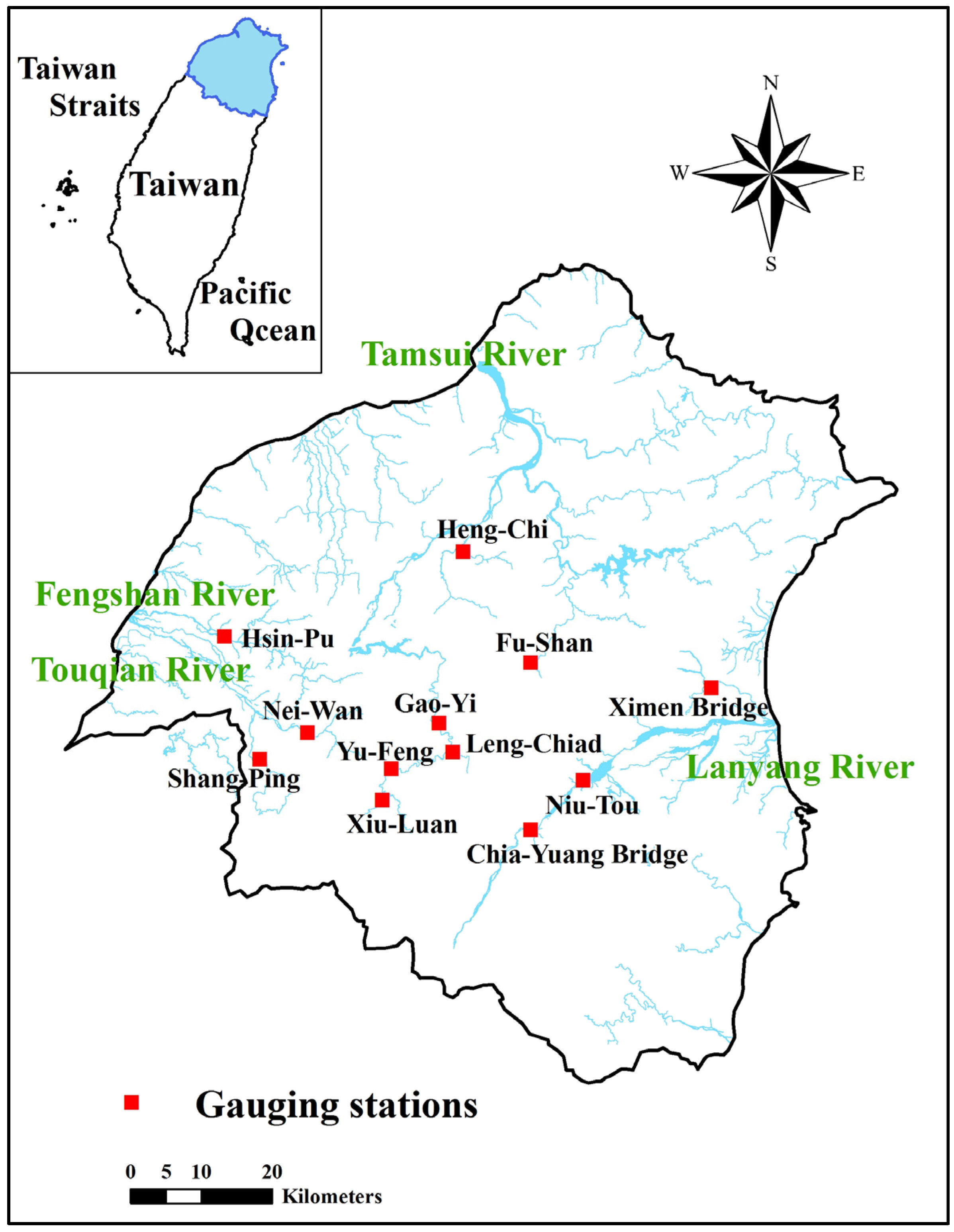
In this study, the long-term streamflow data for the Northern Taiwan regions collected by the Water Resources Agency of the Ministry of Economic Affairs are used for analysis. Data from 12 gauging stations in the Northern Taiwan regions not affected by artificial water conservancy facilities are selected. The geographical locations of the gauging stations are shown in Figure 1.
Figure 1.
Locations of study area and streamflow stations.
4. Results and Discussion
4.1. Results of Average Annual Streamflow Analysis
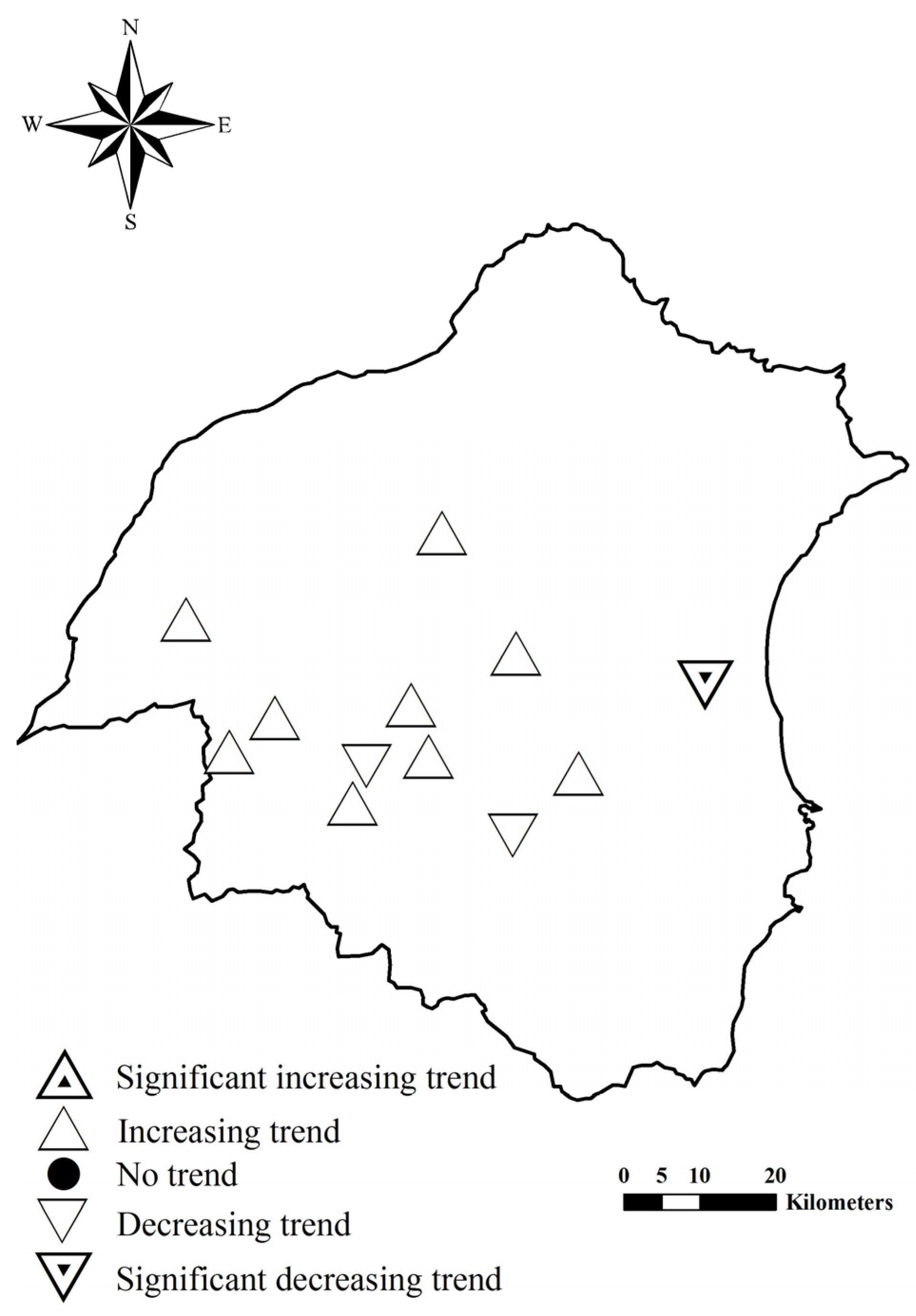
The streamflow trend analysis was conducted using the Mann-Kendall test in order to analyze the average annual streamflow trend significance. The test results are shown in Table 2. To test trend significance, a significance level of α = 0.05 was set as the standard, making . The analysis results show that the Ximen Bridge Station in the Lanyang River basin was the only gauging station exhibiting a significant downward streamflow trend, with a test value of −3.51. Overall, nine of the 12 gauging stations in the study showed an upward streamflow trend, while downward streamflow trends were primarily exhibited in the Lanyang River basin. The streamflow trends in the Tamsui River, the Fengshan River, and the Touqian River basins were mostly increasing. Figure 2 shows the spatial distribution of the trends for each gauging station.
| River | Gauging Station | Record Length | Mann-Kendall Test Result | Slope Estimator | Relative Change Within the Records |
|---|---|---|---|---|---|
| Lanyang River | Niu-Tou | 1979–2010 | 0.89 | 0.158 | 30.3% |
| Chia-Yuang Bridge | 1974–2012 | −0.73 | −0.049 | −9.8% | |
| Ximen Bridge | 1983–2012 | −3.51 * | −0.294 | −85.7% | |
| Tamsui River | Yu-Feng | 1957–2002 | −0.04 | −0.004 | −1.0% |
| Leng-Chiad | 1957–2002 | 0.83 | 0.002 | 1.3% | |
| Fu-Shan | 1953–2012 | 1.89 | 0.063 | 16.7% | |
| Xiu-Luan | 1957–2002 | 0.55 | 0.014 | 10.7% | |
| Gao-Yi | 1957–2002 | 0.15 | 0.010 | 1.5% | |
| Heng-Chi | 1958–2012 | 1.02 | 0.010 | 11.2% | |
| Fengshan River | Hsin-Pu | 1970–2012 | 0.57 | 0.026 | 11.4% |
| Touqian River | Nei-Wan | 1971–2012 | 0.93 | 0.047 | 19.9% |
| Shang-Ping | 1971–2012 | 1.28 | 0.009 | 28.6% |
Note: * indicates the significant trends. The positive values represent increasing trends, and the negative ones represent decreasing trends.
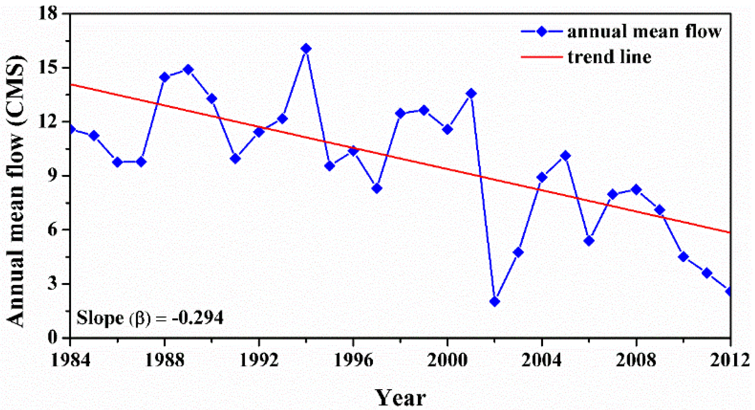
The trend slope calculation was performed using the Theil-Sen estimator, where a trend slope greater (less) than zero indicates an upward (downward) streamflow trend. The trend slope values were also used to create a trend line so as to calculate the annual streamflow. The amount of change in annual streamflow was calculated using Equation (6). The calculation results are shown in Table 2, which reveals that the amount of change in the Tamsui River and the Fengshan River basins (<17.0%) was less than that of the Lanyang River and the Touqian River basins. Of the three gauging stations in the Lanyang River basin, the Niu-Tou Station and the Ximen Bridge Station had significantly greater changes than that of the Chia-Yuang Bridge Station; the Niu-Tou Station showed an upward increase of 30.3%, and the Ximen Bridge Station showed a downward decrease of 85.7%. Concerning the gauging stations in the Touqian River basin, the Nei-Wan Station and the Shang-Ping Station both exhibited an upward increase of 19.9% and 28.6%, respectively. The Ximen Bridge Station trend slope analysis results are shown in Figure 3.
Figure 2.
Map showing spatial variation in trends in annual mean flows.

Figure 3.
Time series plots for the annual mean flow at the Ximen Bridge Station. The straight red line shows the trend line.
Figure 3.
Time series plots for the annual mean flow at the Ximen Bridge Station. The straight red line shows the trend line.

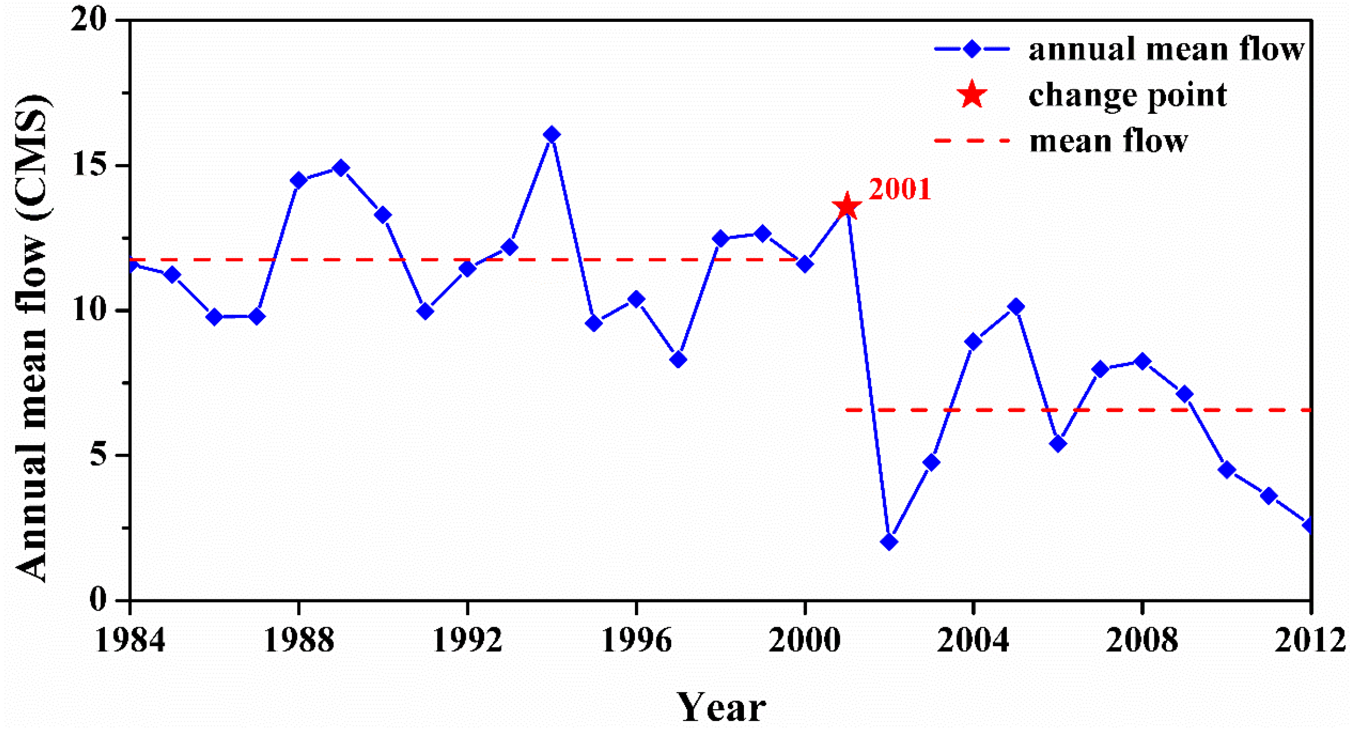
The cumulative deviations and Mann-Whiney-Pettitt statistic tests were calculated to analyze the change points in Table 3. The results of the change point analysis show that change points only Ximen Bridge Station existed in the 12 gauging stations in the study area. The change point of the Ximen Bridge Station occurred in 2001, and the average annual streamflows before and after the change point were 11.8 and 6.6 m3/s, respectively (Figure 4). The average annual streamflow decreased after 2001, and the magnitude of the decrease was 44.1%.
Table 3.
Change points determined by using the cumulative deviations and Mann-Whiney-Pettitt methods.
| River | Gauging Station | Change Points (Year) | Values of (Cumulative Deviations) | Values of p (Mann-Whiney-Pettitt) | The Annual Mean Flow (CMS) | Relative Change at the Change Point | |
|---|---|---|---|---|---|---|---|
| Before Change Point | After Change Point | ||||||
| Lanyang River | Niu-Tou | - | 1.0045 | 0.8640 | - | - | - |
| Chia-Yuang Bridge | - | 0.5633 | 0.5493 | - | - | - | |
| Ximen Bridge | 2001 | 2.0586 | 0.9997 | 11.8 | 6.6 | −44.1% | |
| Tamsui River | Yu-Feng | - | 0.4505 | 0.3269 | - | - | - |
| Leng-Chiad | - | 0.7575 | 0.7285 | - | - | - | |
| Fu-Shan | - | 0.8910 | 1.0634 | - | - | - | |
| Xiu-Luan | - | 0.5859 | 0.4132 | - | - | - | |
| Gao-Yi | - | 0.4496 | 0.3401 | - | - | - | |
| Heng-Chi | - | 0.8304 | 0.8108 | - | - | - | |
| Fengshan River | Hsin-Pu | - | 0.6779 | 0.5634 | - | - | - |
| Touqian River | Nei-Wan | - | 1.0632 | 0.6614 | - | - | - |
| Shang-Ping | - | 0.8907 | 0.7480 | - | - | - | |
Note: The number in bold indicates a statistically significant difference.
Figure 4.
The results for the change points at the Ximen Bridge Station.

4.2. Results of Average Seasonal Streamflow Analysis
The long-term monthly streamflow trend changes were investigated using the gauging station data. The average streamflow of each gauging station from January to December was determined. The Mann-Kendall test results are shown in Table 4. Prior to studying the analysis results, the year was divided into four seasons: spring (March to May), summer (June to August), fall (September to November), and winter (December to February). Approximately 72.2% of the gauging stations in the study area showed an upward streamflow trend in the spring. The majority of these gauging stations were located in the Tamsui River and the Touqian River basins. All of the gauging stations in the Tamsui River drainage basin displayed an upward streamflow trend, while 83.3% of the data samples from the Touqian River basin showed an upward streamflow trend. Conversely, gauging stations exhibiting downward streamflow trends were primarily found in the Lanyang River and the Fengshan River basins, where the percentages of downward streamflow trends were 77.8% and 66.7%, respectively. In the fall, 66.7% of the gauging stations displayed a downward streamflow trend, most of which were found in the Lanyang River, the Tamsui River, and the Fengshan River basins. The downward streamflow trends of the three basins were 66.7%, 77.8%, and 66.7%, respectively. In contrast, most of the gauging stations in the Touqian River basin exhibited an upward streamflow (66.7%). These trend distributions indicate that no significant trend distributions occurred in the summer and winter, while a significant trend distribution transpired in the spring and fall. Upward streamflow trends in the spring were primarily found in the Tamsui River and the Touqian River basins, and downward streamflow trends were mostly found in the Lanyang River and the Fengshan River basins. Upward streamflow trends in the fall were mainly found in the Touqian River basin, and downward streamflow trends were mostly found in the Lanyang River, the Tamsui River, and the Fengshan River basins.
Table 5 shows the relative changes in monthly mean streamflow (in percentages) using trend slope calculations. In spring, the change ratios of the Tamsui River basin were greater than those of other basins, which exhibited a general upward streamflow trend in which over 38.9% of the data samples demonstrated change ratios of monthly mean streamflow of more than 40%. Table 6 shows the results of the monthly change point test. Of the 13 change points identified, the majority of them occurred prior to 2000, with six change points appearing after 2000. The Ximen Bridge Station in the Lanyang River basin showed a decreasing streamflow trend after the change point, while the Yu-Feng Station, the Xiu-Luan Station, and the Heng-Chi Station in the Tamsui River basin displayed an upward streamflow trend. In terms of change point distribution, seven of the 13 change points occurred in the spring; they were also primarily found in the Tamsui River and the Lanyang River basins. Concerning the change points of the Tamsui River basin, the average streamflow exhibited an upward streamflow trend after the change point. In contrast, in the case of the Lanyang River basin, the average streamflow showed a downward streamflow trend after the change point.
4.3. Results of the High and Low Streamflow Analysis
First, the daily average streamflow data were ranked before being divided into 10 equal portions and nine threshold values. The nine threshold values were Q0.1, Q0.2, …, Q0.9. The streamflow data corresponding to Q0.1, Q0.2, …, Q0.9 were analyzed using the Mann-Kendall test. The high and low flows (Q0.9 and Q0.1) were then analyzed for the purpose of discussion.
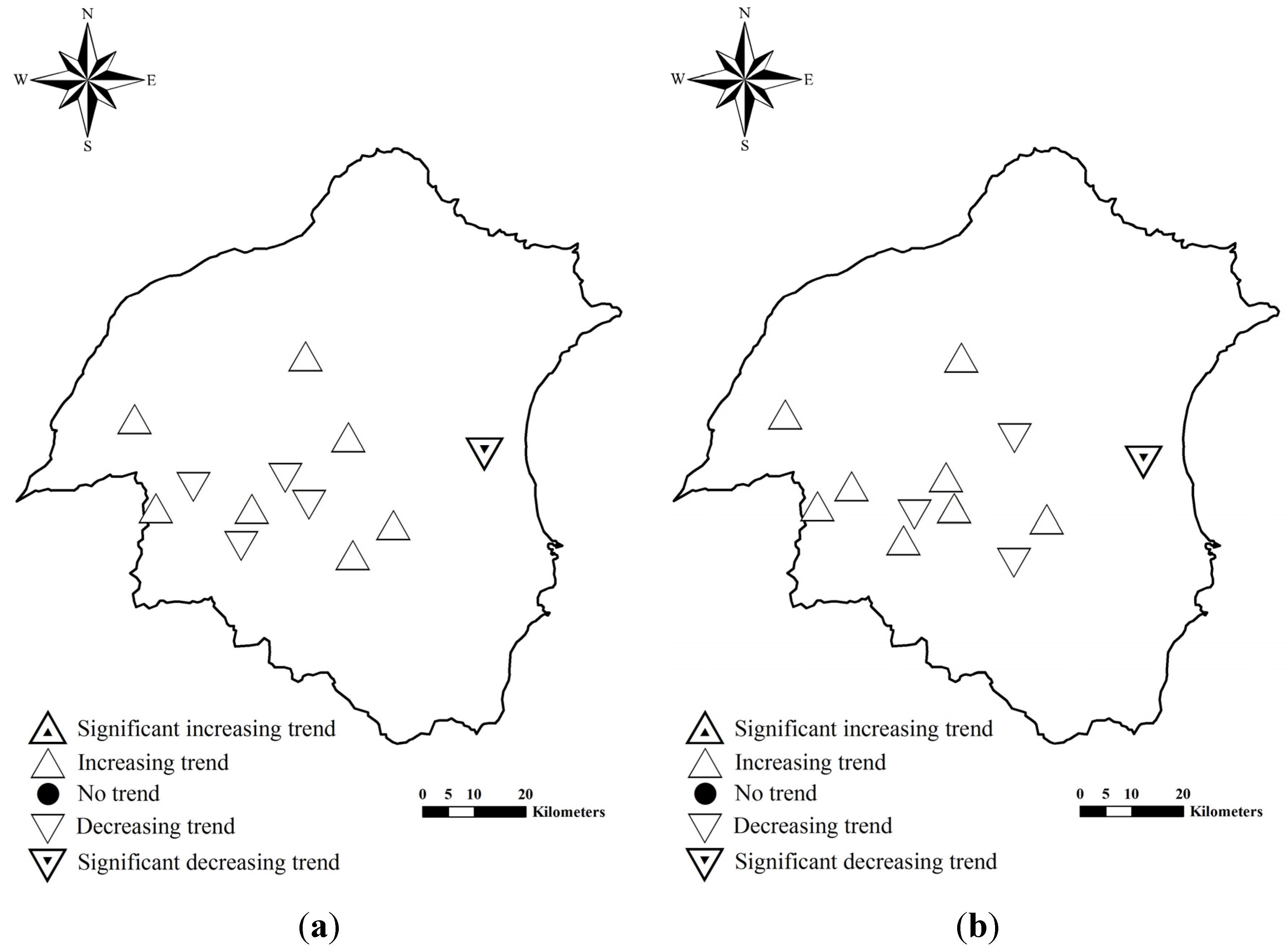
Table 7 presents the high and low flow data obtained using the Mann-Kendall test, which show that the Ximen Bridge Station was the only gauging station to feature a significant downward streamflow trend for both high and low flows. The high flow test results (Q0.9) show that of the 12 gauging stations, eight showed an upward streamflow trend, and only four displayed a downward streamflow trend (Figure 5). The Tamsui River, the Fengshan River, and the Touqian River basins mainly exhibited an upward streamflow trend; of the six gauging stations in the Tamsui River basin, four showed an upward streamflow trend, and all the gauging stations in the Fengshan River and Touqian River basins demonstrated an upward streamflow trend. In contrast, most (two of three) of the gauging stations in the Lanyang River basin showed a downward streamflow trend. Regarding low flow (Q0.1), the test results revealed that seven of the 12 gauging stations featured upward streamflow trends, while the remaining five gauging stations demonstrated downward streamflow trends (Figure 5). However, no significant spatial distribution was observed for any of the 12 gauging stations.
| Gauging Station | River | Spring | Summer | Fall | Winter | ||||||||
|---|---|---|---|---|---|---|---|---|---|---|---|---|---|
| March | April | May | June | July | August | September | October | November | December | January | February | ||
| Niu-Tou | Lanyang River | −0.341 | −0.146 | −0.632 | 0.308 | 1.638 | −0.016 | 0.600 | 1.573 | 0.405 | 0.892 | 0.243 | 0.114 |
| Chia-Yuang Bridge | 0.470 | 0.730 | −0.016 | −0.859 | 1.573 | −0.600 | −1.508 | −0.341 | −0.730 | 1.443 | 0.438 | 0.957 | |
| Ximen Bridge | −2.345 * | −3.395 * | −3.733 * | −3.320 * | −1.332 | −1.557 | −2.757 * | −1.332 | −2.195 * | −2.607 * | −3.170 * | −3.095 * | |
| Yu-Feng | Tamsui River | 0.701 | 1.800 | 2.103 * | −0.815 | −0.322 | 0.114 | −0.758 | −0.739 | 0.019 | −0.360 | −0.720 | 0.303 |
| Leng-Chiad | 0.578 | 1.374 | 1.108 | −0.123 | −0.256 | 0.047 | −0.066 | −0.218 | −0.142 | −0.521 | −1.165 | 0.379 | |
| Fu-Shan | 0.184 | 1.941 | 1.539 | 0.535 | 0.803 | 0.552 | 0.502 | −0.033 | −1.188 | −0.786 | −0.987 | 0.535 | |
| Xiu-Luan | 0.966 | 2.406 * | 2.198 * | 0.171 | −0.474 | 0.265 | −0.398 | −0.398 | −0.834 | −0.834 | −0.739 | 0.587 | |
| Gao-Yi | 0.739 | 1.895 | 1.914 | −0.493 | −0.493 | 0.095 | −0.815 | −0.758 | −0.493 | −1.269 | −1.421 | 0.512 | |
| Heng-Chi | 0.951 | 2.035 * | 0.738 | −1.111 | 0.204 | 1.040 | 0.133 | 0.187 | −0.169 | 1.307 | −0.915 | 1.075 | |
| Hsin-Pu | Fengshan River | −0.105 | 0.523 | −0.356 | −0.042 | 1.026 | −0.335 | −0.126 | 0.795 | −0.105 | 0.000 | −0.649 | 0.544 |
| Nei-Wan | Touqian River | −0.412 | 0.325 | 1.019 | −0.217 | 0.954 | 0.108 | 1.713 | −0.260 | 1.279 | 0.369 | −1.019 | 0.260 |
| Shang-Ping | 0.390 | 0.737 | 0.238 | −0.629 | 1.279 | 0.195 | 0.542 | −0.455 | 1.127 | 0.499 | −0.824 | −0.043 | |
Note: * indicates the significant trends. The positive values represent increasing trends, and the negative ones represent decreasing trends.
| Gauging Station | River | Spring | Summer | Fall | Winter | ||||||||
|---|---|---|---|---|---|---|---|---|---|---|---|---|---|
| March | April | May | June | July | August | September | October | November | December | January | February | ||
| Niu-Tou | Lanyang River | −6.9% | −3.7% | −16.6% | 5.4% | 51.8% | 0.02% | 20.8% | 79.2% | 8.9% | 18.6% | 5.7% | 0.7% |
| Chia-Yuang Bridge | 9.3% | 25.2% | 0.7% | −23.2% | 57.3% | −22.2% | −49.5% | −13.0% | −16.4% | 36.3% | 7.7% | 26.0% | |
| Ximen Bridge | −86.0% | −115.5% | −113.7% | −107.1% | −39.1% | −57.4% | −101.8% | −38.8% | −73.9% | −102.3% | −109.6% | −109.0% | |
| Yu-Feng | Tamsui River | 17.3% | 46.6% | 48.4% | −19.1% | −4.8% | 1.3% | −22.7% | −12.5% | 1.1% | −8.3% | −8.3% | 7.4% |
| Leng-Chiad | 11.3% | 35.2% | 25.6% | −0.9% | −6.3% | 1.6% | −0.8% | −2.6% | −4.1% | −11.1% | −23.7% | 6.0% | |
| Fu-Shan | 3.3% | 39.6% | 35.9% | 9.4% | 21.7% | 11.8% | 18.8% | −0.8% | −21.3% | −14.3% | −18.5% | 12.0% | |
| Xiu-Luan | 26.5% | 67.9% | 57.0% | 4.2% | −9.9% | 5.9% | −9.5% | −7.6% | −17.4% | −15.8% | −10.8% | 11.6% | |
| Gao-Yi | 14.9% | 47.6% | 46.9% | −8.2% | −12.6% | 4.8% | −31.7% | −16.5% | −9.9% | −21.0% | −22.1% | 9.7% | |
| Heng-Chi | 26.0% | 62.8% | 23.7% | −26.5% | 7.8% | 36.4% | 6.3% | 4.0% | −4.4% | 32.2% | −28.8% | 42.4% | |
| Hsin-Pu | Fengshan River | −6.5% | 16.4% | −9.9% | −0.3% | 31.6% | −9.8% | −1.9% | 20.2% | −2.0% | 0.5% | −21.2% | 11.7% |
| Nei-Wan | Touqian River | −14.2% | 9.8% | 25.6% | −7.8% | 25.9% | 3.4% | 49.2% | −7.1% | 26.5% | 4.6% | −33.3% | 5.2% |
| Shang-Ping | 7.3% | 21.4% | 5.5% | −17.7% | 43.6% | 4.7% | 14.6% | −6.3% | 26.4% | 6.2% | −25.8% | −1.9% | |
Note: The positive values represent increasing trends, and the negative ones represent decreasing trends.
| Gauging Station | River | Spring | Summer | Fall | Winter | ||||||||
|---|---|---|---|---|---|---|---|---|---|---|---|---|---|
| March | April | May | June | July | August | September | October | November | December | January | February | ||
| Niu-Tou | Lanyang River | ||||||||||||
| Chia-Yuang Bridge | |||||||||||||
| Ximen Bridge | 2001 | 1999 | 1997 | 2001 | 1994 | 2001 | 2004 | 2001 | 2001 | ||||
| Yu-Feng | Tamsui River | 1973 | |||||||||||
| Leng-Chiad | |||||||||||||
| Fu-Shan | |||||||||||||
| Xiu-Luan | 1977 | 1973 | |||||||||||
| Gao-Yi | |||||||||||||
| Heng-Chi | 1972 | ||||||||||||
| Hsin-Pu | Fengshan River | ||||||||||||
| Nei-Wan | Touqian River | ||||||||||||
| Shang-Ping | |||||||||||||
| River | Gauging Station | High Flow (Q0.9) | Low Flow (Q0.1) |
|---|---|---|---|
| Mann-Kendall Test Result | Mann-Kendall Test Result | ||
| Lanyang River | Niu-Tou | 0.778 | 0.876 |
| Chia-Yuang Bridge | −0.146 | 0.535 | |
| Ximen Bridge | −3.995 * | −2.739 * | |
| Tamsui River | Yu-Feng | −0.142 | 0.464 |
| Leng-Chiad | 1.203 | −0.275 | |
| Fu-Shan | −0.008 | 1.497 | |
| Xiu-Luan | 0.872 | −0.711 | |
| Gao-Yi | 0.057 | −0.180 | |
| Heng-Chi | 1.111 | 1.653 | |
| Fengshan River | Hsin-Pu | 0.910 | 0.073 |
| Touqian River | Nei-Wan | 0.683 | −0.954 |
| Shang-Ping | 1.420 | 0.217 |
Note: * indicates the significant trends. The positive values represent increasing trends, and the negative ones represent decreasing trends.
Figure 5.
Maps showing spatial variation in trends in high and low flows: (a) high flow; (b) low flow.
Figure 5.
Maps showing spatial variation in trends in high and low flows: (a) high flow; (b) low flow.

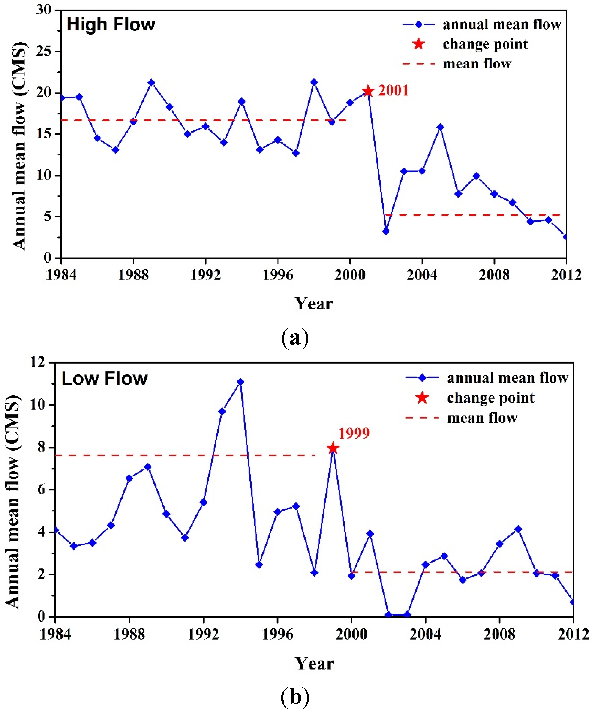
Results for the high and low flow trend slope analysis are shown in Table 8. Concerning high flow (Q0.9), gauging stations with a change ratio of greater than 20% included the Niu-Tou Station and the Ximen Bridge Station in the Lanyang River basin, the Hsin-Pu Station in the Fengshan River basin, and the Shang-Ping Station in the Touqian River basin. The Niu-Tou Station showed an upward streamflow trend (21.3%); the Ximen Bridge Station displayed a downward streamflow trend (−103.5%); the Hsin-Pu Station displayed an upward streamflow trend (22.9%); and the Shang-Ping Station demonstrated an upward streamflow trend (24.3%). Regarding low flow (Q0.1), gauging stations with a change ratio greater than 20% were the Ximen Bridge Station in the Lanyang River basin, the Nei-Wan Station in the Touqian River basin, and the Fu-Shan Station and the Heng-Chi Station in the Tamsui River basin. The Ximen Bridge Station and the Nei-Wan Station both showed a downward streamflow trend (−82.5% and −34.8%, respectively). Conversely, the Fu-Shan Station and the Heng-Chi Station both displayed an upward streamflow trend (20.7% and 26.7%, respectively). The high and low flow change point test analysis shows that the Ximen Bridge Station was the only gauging station of the 12 gauging stations to feature a change point, with high and low flow change points occurring in 2001 and 1999, respectively (Figure 6). A downward streamflow trend was observed after both change points, where the changes were significant. The high flows before and after the change point were 16.7 and 7.6 cms, respectively, showing a change ratio of −54.2%. The low streamflows before and after the change point were 5.2 and 2.1 cms, respectively, indicating a change ratio of −59.4%.
| Gauging Station | High Flow (Q0.9) | Low Flow (Q0.1) | ||||
|---|---|---|---|---|---|---|
| Slope Estimator | Mean High Flow (CMS/Year) | Relative Change within the Records (CMS/Year) | Slope Estimator | Mean Low Flow (CMS/year) | Relative Change within the Records (CMS/Year) | |
| Niu-Tou | 0.155 | 22.6 | 21.3% | 0.011 | 1.8 | 19.2% |
| Chia-Yuang Bridge | −0.026 | 22.2 | −3.7% | 0.017 | 5.0 | 10.8% |
| Ximen Bridge | −0.494 * | 13.4 * | −103.5% | −0.116 * | 3.9 * | −82.5% |
| Yu-Feng | −0.007 | 24.9 | −1.3% | 0.007 | 4.3 | 7.5% |
| Leng-Chiad | 0.000 | 10.1 | 19.0% | −0.001 | 2.2 | −2.7% |
| Fu-Shan | 0.000 | 25.9 | 0.0% | 0.026 | 5.9 | 20.7% |
| Xiu-Luan | 0.029 | 8.7 | 14.8% | −0.003 | 1.1 | −11.5% |
| Gao-Yi | 0.014 | 43.0 | 1.4% | −0.004 | 7.6 | −2.2% |
| Heng-Chi | 0.026 | 6.7 | 18.1% | 0.003 | 0.5 | 26.7% |
| Hsin-Pu | 0.084 | 15.3 | 22.9% | 0.001 | 0.8 | 3.0% |
| Nei-Wan | 0.026 | 15.4 | 6.9% | −0.014 | 1.6 | −34.8% |
| Shang-Ping | 0.140 | 23.6 | 24.3% | 0.002 | 2.8 | 3.4% |
Note: * indicates the significant trends. The positive values mean the increasing trends and the negative ones mean the decreasing trends.
Figure 6.
Results for the change points in the high and low flows: (a) high flow; (b) low flow.

5. Conclusions
In this study, the streamflow data from 12 gauging stations in Northern Taiwan regions were obtained, and their trend changes were analyzed using the Mann-Kendall test. The trend slopes were calculated, and the change points were analyzed. The following conclusions were reached:
- (1)
- Based on the results of the average annual streamflow analysis, only the Ximen Bridge Station in the Lanyang River basin exhibited significant downward streamflow trends, while the rest of the gauging stations featured no significant upward or downward streamflow trends. In terms of overall trends, upward streamflow trends were primarily found in the Tamsui River, the Fengshan River, and the Touqian River basins, whereas downward streamflow trends were mostly observed in the Lanyang River drainage basin. The results of the trend slope analysis revealed that the amount of change in the Tamsui River and the Fengshan River basins was less than that in the Lanyang River and the Touqian River basins. The Ximen Bridge Station was the only station which had a change point.
- (2)
- The results of the monthly and seasonal average streamflow analysis show that in the spring, 72.2% of the gauging stations showed upward streamflow trends, most of which were located in the Tamsui River and the Touqian River basins. All of the gauging stations in the Tamsui River basin displayed upward streamflow trends, while 83.3% of the data samples from the Touqian River basin showed an upward streamflow trend. Conversely, gauging stations exhibiting downward streamflow trends were primarily found in the Lanyang River and Fengshan River basins. The percentage of the downward streamflow trend in the Lanyang River basins was remarkably high (77.8%). The results of the change point test showed that seven of the 13 change points occurred in the spring and were mostly found in the Tamsui River and the Lanyang River basins, where the average streamflow increased and decreased for the former and the latter, respectively.
- (3)
- The high and low flow data analysis showed that the Ximen Bridge Station was the only gauging station to feature a significant downward streamflow trend in the case of both high and low flows. The results of the high flow tests (Q0.9) revealed that the Tamsui River, the Fengshan River, and the Touqian River basins primarily demonstrated upward streamflow trends, while the Lanyang River basin mainly displayed downward streamflow trends. The results of the low flow tests (Q0.1) indicated that 58.3% of the gauging stations showed an upward streamflow trend; however, no significant trend distribution was observed. The change point test analysis showed that the Ximen Bridge Station was the only gauging station of the 12 gauging stations to feature a change point, with the high and low flow change points occurring in 2001 and 1999, respectively. A downward streamflow trend was observed after both change points had occurred, and the changes were significant.
Acknowledgments
The authors are grateful for the support of the Research Project of the Ministry of Science and Technology (MOST 103-2221-E-006-205-MY2).
Author Contributions
Chen-Feng Yeh conceived the subject of the article, literature review and contributed to the writing of the paper; Jinge Wang participated in data processing, elaborated the statistical analysis, and figures. Hsin-Fu Yeh and Cheng-Haw Lee participated in the composition of the manuscript in the method, results and conclusion sections.
Conflicts of Interest
The authors declare no conflict of interest.
References
- Nicholls, R.J.; Cazenave, A. Sea-level rise and its impact on coastal zones. Science 2010, 328, 1517–1520. [Google Scholar] [CrossRef] [PubMed]
- Dams, J.; Salvadore, E.; van Daele, T.; Ntegeka, V.; Willems, P.; Batelaan, O. Spatio-temporal impact of climate change on the groundwater system. Hydrol. Earth Syst. Sci. 2012, 16, 1517–1531. [Google Scholar] [CrossRef] [Green Version]
- Huang, J.C.; Lee, T.Y.; Lee, J.Y. Observed magnified runoff response to rainfall intensification under global warming. Environ. Res. Lett. 2014, 9, 034008. [Google Scholar] [CrossRef]
- Liang, L.; Liu, Q. Streamflow sensitivity analysis to climate change for a large water-limited basin. Hydrol. Process. 2014, 28, 1767–1774. [Google Scholar] [CrossRef]
- Lins, H.F.; Slack, J.R. Streamflow trends in the United States. Geophys. Res. Lett. 1999, 26, 227–230. [Google Scholar] [CrossRef]
- Zhang, X.; Harvey, K.D.; Hogg, W.D.; Yuzyk, T.R. Trends in Canadian streamflow. Water Resour. Res. 2001, 37, 987–998. [Google Scholar] [CrossRef]
- Kahya, E.; Kalayci, S. Trend analysis of streamflow in Turkey. J. Hydrol. 2004, 289, 128–144. [Google Scholar] [CrossRef]
- Chen, Z.; Chen, Y.; Li, B. Quantifying the effects of climate variability and human activities on runoff for Kaidu River Basin in arid region of northwest China. Theor. Appl. Climatol. 2013, 111, 537–545. [Google Scholar] [CrossRef]
- Dixon, H.; Lawler, D.M.; Shamseldin, A.Y. Streamflow trends in western Britain. Geophys. Res. Lett. 2006, 33, L19406. [Google Scholar] [CrossRef]
- Baggaley, N.J.; Langan, S.J.; Futter, M.N.; Potts, J.M.; Dunn, S.M. Long-term trends in hydro-climatology of a major Scottish mountain river. Sci. Total Environ. 2009, 407, 4633–4641. [Google Scholar] [CrossRef] [PubMed]
- Hannaford, J.; Buys, G. Trends in seasonal river flow regimes in the UK. J. Hydrol. 2012, 475, 158–174. [Google Scholar] [CrossRef] [Green Version]
- Bassiouni, M.; Oki, D.S. Trends and shifts in streamflow in Hawai’i, 1913–2008. Hydrol. Process. 2013, 27, 1484–1500. [Google Scholar] [CrossRef]
- De Martino, G.; Fontana, N.; Marini, G.; Singh, V.P. Variability and trend in seasonal precipitation in the continental United States. J. Hydrol. Eng. 2013, 18, 630–640. [Google Scholar] [CrossRef]
- Duhan, D.; Pandey, A. Statistical analysis of long term spatial and temporal trends of precipitation during 1901–2002 at Madhya Pradesh, India. Atmos. Res. 2013, 122, 136–149. [Google Scholar] [CrossRef]
- Pasquini, A.I.; Depetris, P.J. Discharge trends and flow dynamics of South American rivers draining the southern Atlantic seaboard: An overview. J. Hydrol. 2007, 333, 385–399. [Google Scholar] [CrossRef]
- Ngongondo, C.S. An analysis of long-term rainfall variability, trends and groundwater availability in the Mulunguzi river catchment area, Zomba mountain, Southern Malawi. Quat. Int. 2006, 148, 45–50. [Google Scholar] [CrossRef]
- Rouge, C.; Ge, Y.; Cai, X. Detecting gradual and abrupt changes in hydrological records. Adv. Water Resour. 2013, 53, 33–44. [Google Scholar] [CrossRef]
- Yu, P.S.; Yand, T.C.; Kuo, C.C. Evaluating long-term trends in annual and seasonal precipitation in Taiwan. Water Resour. Manag. 2006, 20, 1007–2023. [Google Scholar] [CrossRef]
- Water Resources Agency (WRA). Hydrological Year Book of Taiwan; Ministry of Economic Affairs: Taipei, Taiwan, 2013.
- Kendall, M.G. Rank Correlation Methods; Charles Griffin: London, UK, 1975. [Google Scholar]
- Mann, H.B. Non-parametric test against trend. Econometrica 1945, 13, 245–259. [Google Scholar] [CrossRef]
- Sen, P.K. Estimates of the regression coefficient based on Kendall’s tau. J. Am. Stat. Assoc. 1968, 63, 1379–1389. [Google Scholar] [CrossRef]
- Petrow, T.; Merz, B. Trends in flood magnitude, frequency and seasonality in Germany in the period 1951–2002. J. Hydrol. 2009, 371, 129–141. [Google Scholar] [CrossRef]
- Pettit, A.N. A non-parametric approach to the change point problem. J. R. Stat. Soc. Ser. C 1979, 28, 126–135. [Google Scholar]
- Buishand, T.A. Some methods for testing the homogeneity of rainfall records. Hydrol. Process. 1982, 314, 312–329. [Google Scholar]
© 2015 by the authors; licensee MDPI, Basel, Switzerland. This article is an open access article distributed under the terms and conditions of the Creative Commons Attribution license (http://creativecommons.org/licenses/by/4.0/).
Share and Cite
MDPI and ACS Style
Yeh, C.-F.; Wang, J.; Yeh, H.-F.; Lee, C.-H. Spatial and Temporal Streamflow Trends in Northern Taiwan. Water 2015, 7, 634-651. https://doi.org/10.3390/w7020634
AMA Style
Yeh C-F, Wang J, Yeh H-F, Lee C-H. Spatial and Temporal Streamflow Trends in Northern Taiwan. Water. 2015; 7(2):634-651. https://doi.org/10.3390/w7020634
Chicago/Turabian StyleYeh, Chen-Feng, Jinge Wang, Hsin-Fu Yeh, and Cheng-Haw Lee. 2015. "Spatial and Temporal Streamflow Trends in Northern Taiwan" Water 7, no. 2: 634-651. https://doi.org/10.3390/w7020634