Modelling the Hydraulic Behaviour of Growing Media with the Explicit Finite Volume Solution

Abstract

The increasing imperviousness of urban areas reduces the infiltration and evapotranspiration capacity of urban catchments and results in increased runoff. In the last few decades, several solutions and techniques have been proposed to prevent such impacts by restoring the hydrological cycle. A limiting factor in spreading the use of such systems is the lack of proper modelling tools for design, especially for the infiltration processes in a growing medium. In this research, a physically-based model, employing the explicit Finite Volume Method (FVM), is proposed for modelling infiltration into growing media. The model solves a modified version of the Richards equation using a formulation which takes into account the main characteristics of green infrastructure substrates. The proposed model was verified against the HYDRUS-1D software and the comparison of results confirmed the suitability of the proposed model for correctly describing the hydraulic behaviour of soil substrates.

1. Introduction

Progressing urbanization of undeveloped land leads to an increasing amount of impervious surfaces at the expense of natural areas. Leopold [1], while describing the effects of urbanization on the hydrological cycle, identified such major effects as reduced infiltration and evapotranspiration, resulting in increased runoff and reduced groundwater recharge. Traditional stormwater management design focused on collecting stormwater in piped networks and transporting it off-site as quickly as possible. Increases in the incidence of flooding and combined sewer overflows (CSOs) in urban areas demonstrate that the traditional approach is inadequate for managing stormwater. Conversely, the Low Impact Development (LID) approach aims to preserve and restore natural features, minimize the imperviousness of urban catchments, and increase their infiltration and evapotranspiration capacities. LID techniques include bio-retention cells, grass swales, porous pavements, green roofs, and many other measures.

Considering that rooftops may represent 40%–50% of impervious surfaces in urban areas, green roofs are among the key options for hydrologic restoration and stormwater management.

Green roofs (GR) consist of a number of layers, including a vegetation layer, a lightweight soil medium, a drainage layer and an impermeable membrane. The soil medium and drainage layer are the most crucial elements in a green roof. The primary functions of a drainage layer are to remove excess rain water but still retain some amount of water, while being light and thin. Recent studies have focused on the optimization of the drainage layer for the removal of nutrients released from the growing medium of a green roof during rainfall events [2]. On the other hand, the hydraulic behaviour of a green roof is strongly influenced by the characteristics of the growing medium, which must be highly permeable, in order to avoid ponding of water on the GR surface. Ponding adds excess weight load, can float and scour substrate, and can potentially drown plants. Organic matter in the substrate increases the retention capacity of the green roof but decreases its permeability.

Studies of the hydraulic/hydrologic performance of green roofs reported excellent results: green roofs were able to significantly reduce storm-water runoff and retain rainfall volume with retention efficiencies ranging from 40% to 80% [3], and green roofs reduced storm-water runoff peak rates by 60%–80% [4].

In spite of the large and well-known benefits of green roofs and other LID techniques, the transition to sustainable urban drainage systems is very slow [5]. One of the key limiting factors in the widespread adoption of such systems is the lack of adequate analytical and modelling tools [6].

The infiltration process in the GR soil substrate is one of the most critical aspects in GR modelling. Various models describing the infiltration process have been developed and presented in the literature, with empirical relationships, the rational method, cascades of linear reservoirs, and the US Soil Conservation Service Curve Number method being used most frequently. Physically-based models are not widely used, even though they are well-suited for GR planning and design [7] and may be more accurate than the conceptual and empirical models. The physically-based models are typically based on numerical solutions of the Richards equation [8] for the description of the unsaturated flow in the porous matrix of the GR. The Richards equation is an elliptic-parabolic partial differential equation, for which no general analytical solution exists, so numerical approximations must be used (e.g., the Finite Element Method, Finite Volume Method, etc.). This represents one of the barriers to a broader adoption of physically-based models for the analysis of GRs. These considerations and discussion on the topic suggest that there is a research need to develop accurate physically-based models that are easy to implement; this will contribute to more widespread GR applications in urban drainage systems.

The main objective of the paper that follows is to develop a physically-based model of the coarse porous matrix of green roofs, describing the unsaturated flow in the porous medium and its hydraulic behaviour. The model must conserve mass, and it must be computationally efficient and easy to implement.

Even though they are of great interest, processes like evapotranspiration, root water uptake and nutrient leaching have not been considered in this paper because they are beyond the scope of this research, which is mainly focused on the development of a physical model for the study of unsaturated flow in green roof substrates.

2. Materials and Methods

2.1. Mathematical Model and Governing Equation

Flow in a variably saturated porous medium can be described by the Richards equation [8], which can be written as:

$$\frac{\partial \text{θ}(\text{ψ})}{\partial t}-\nabla \cdot K(\text{θ}(\text{ψ}))\nabla (\text{ψ}-z)=0$$

(1)

where θ is the water content (L³/L³), ψ is the suction head (L), K is the unsaturated hydraulic conductivity (L/T), t is the time (T) and z is the depth (L) (positive downward). The Richards equation can be derived by combining two physical laws:

-

The continuity equation, written in its differential form:

$$\frac{\partial \text{θ}(\text{ψ})}{\partial t}+\nabla q=0$$

(2)

where q is the liquid flow, and

-

the Darcy law:

$$q=-K(\text{θ}(\text{ψ}))\nabla (\text{ψ}-z)$$

(3)

The Richards equation may be written in three different forms:

$$\frac{\partial \text{θ}}{\partial t}-\nabla \cdot K(\text{ψ})\nabla (\text{ψ}-z)=0\text{ mixed-form}$$

(4)

$$C(\text{ψ})\frac{\partial \text{ψ}}{\partial t}-\nabla \cdot K(\text{ψ})\nabla (\text{ψ}-z)=0\text{ pressure-form}$$

(5)

$$\frac{\partial \text{θ}}{\partial t}-\nabla \cdot D(\text{θ})\nabla \text{θ}+\nabla K(\text{θ})=0\text{ moisture-form}$$

(6)

where C(ψ) is the hydraulic capacity function (1/L) and D(θ) is the soil water diffusivity (L²/T). The main advantage of the moisture-based form is that it is expressed in terms of the conserved variable. The pressure-based form can handle discontinuities in the porous media, but may lead to significant mass balance errors. The mixed form can conserve mass, and allows for saturated flows and heterogeneity in the porous medium.

Mathematically, the Richards equation has the characteristics of an advection-diffusion equation. It contains a diffusive term associated with soil water diffusivity and an advective term associated with the depth z. These characteristics emerge if we apply a Kirchhoff transformation to the pressure-form of the Richards equation. The Kirchhoff transformation introduces a new variable u:

$$u=u(\text{ψ})={\displaystyle {\int }_{{\text{ψ}}_{\text{max}}}^{\text{ψ}}K(\text{ψ})\text{ dψ}}$$

(7)

This is equivalent to:

$$\frac{\partial u}{\partial z}=K(\text{ψ})\frac{d\text{ψ}}{dz}$$

(8)

By substituting Equation (8) into Equation (6) the following equation is obtained:

$$\frac{\partial u}{\partial t}+v(u)\frac{\partial u}{\partial z}-D(u)\frac{{\partial }^{2}u}{\partial z^2}=0$$

(9)

where D(u) is the soil moisture diffusivity and v(u) is the soil moisture velocity, defined as:

$$D(u)=\frac{K[\text{ψ}(u)]}{C[\text{ψ}(u)]}$$

(10)

$$v(u)=\frac{1}{C[\text{ψ}(u)]}\frac{dK[\text{ψ}(u)]}{d\text{ψ}}=\frac{dK[\text{ψ}(u)]}{d\text{θ}}$$

(11)

The transformed Richards Equation (9) is an advection-diffusion equation where an advective term, associated with the soil moisture velocity v, and a diffusive term, associated with the soil moisture diffusivity D, are clearly highlighted.

Unsaturated Soil Constitutive Models

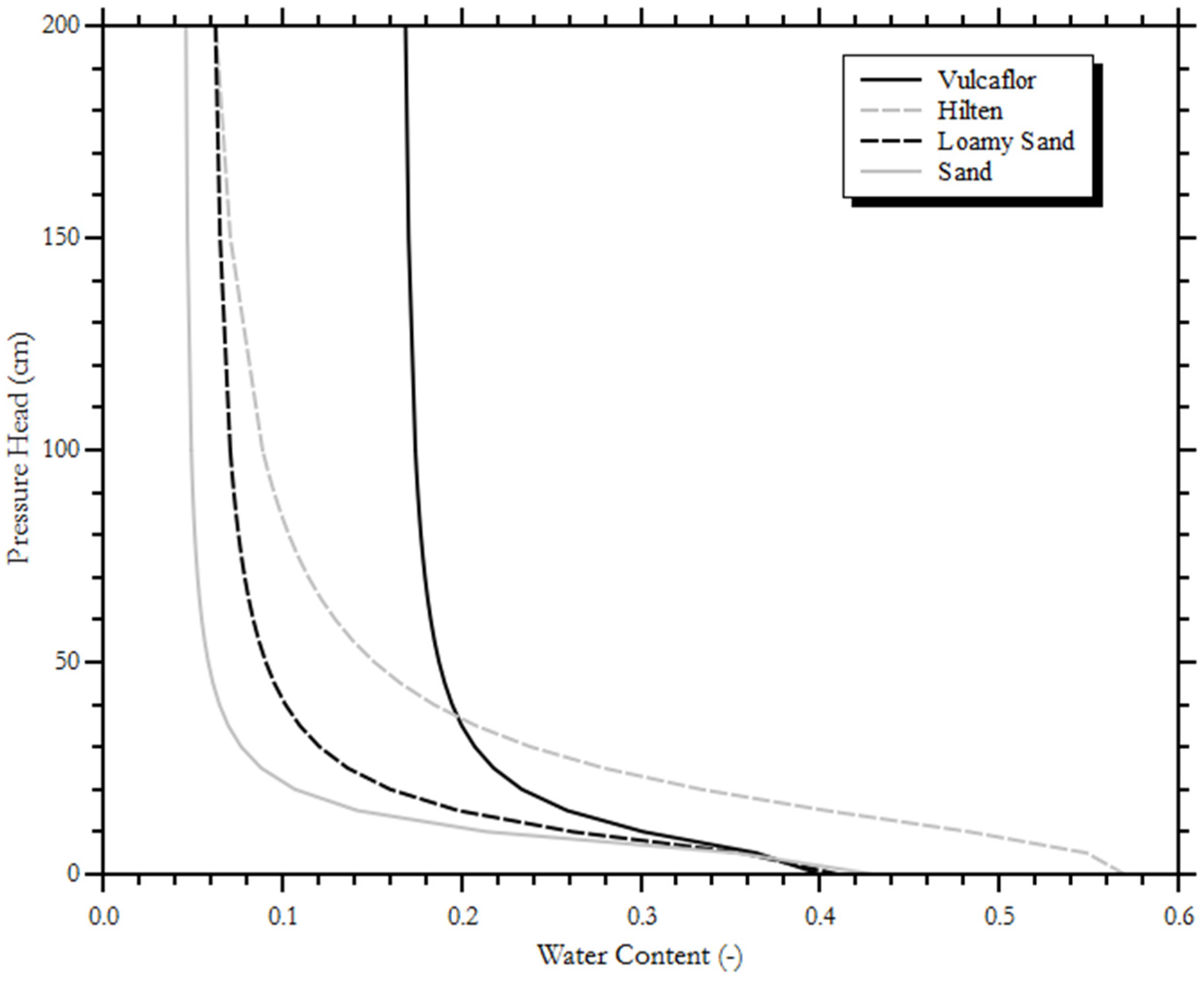
This work builds on the Mualem-van Genuchten (MG) model [9], which is used to define water content θ(ψ) and unsaturated hydraulic conductivity K(θ) (Figure 1). The MG model is used herein, because of its widespread use in the literature and general reliability. The MG model can be expressed as:

$$\text{θ}=\{\begin{array}{c}\frac{{\text{θ}}_s-{\theta }_r}{{(1+{(\text{α}\left|\text{ψ}\right|)}^n)}^m}+{\text{θ}}_r \text{if} \text{ψ}\le 0\\ {\text{θ}}_s \text{if ψ}>0\end{array}$$

(12)

$$S_e=\frac{\text{θ}-{\text{θ}}_r}{{\text{θ}}_s-{\text{θ}}_r}$$

(13)

$$K=\{\begin{array}{c}{K}_s{S}_e^L{\left[{(1-(1-S_e^{\frac{1}{m}})}^m\right]}^2 \text{if ψ}\le 0\\ K_s \text{if ψ}>0\end{array}$$

(14)

$$C=\{\begin{array}{c}\frac{\partial \text{θ}}{\partial \text{ψ}}=-mn{\text{α}}^n\frac{{\text{θ}}_{\mathrm{s}}-{\text{θ}}_r}{{(1+{\text{α}}^n{\left|\text{ψ}\right|}^n)}^{m+1}}{\left|\text{ψ}\right|}^n{\text{ψ}}^{-1} \text{if ψ}\le 0\\ 0 \text{if ψ}>0\end{array}$$

(15)

$$m=1-\frac{1}{n}$$

(16)

where θ_r (L³/L³) is the residual water content, θ_s (L³/L³) is the saturated water content, K_s (L/T) is the saturated hydraulic conductivity, n is a parameter which measures pore-size distribution and α (L⁻¹) is a parameter related to the inverse of the air-entry pressure. L indicates the tortuosity and is usually assumed to be L = 0.5 [10]. S_e is the effective saturation (L³/L³).

Figure 1. Mualem-van Genuchten soil model.

Figure 1. Mualem-van Genuchten soil model.

2.2. Numerical Model

As stated in the introduction, the main purpose of this research is to develop a numerical model that conserves mass and is robust, computationally efficient and easy to implement. Most of the existing models are based on numerical approximations of the Richards equation, which has no general analytical solution. The techniques employed include the Finite Difference method (FDM) [11]; the Finite Element Method (FEM) [12,13]; and the Finite Volume Method (FVM) [14,15,16,17,18]. The use of the FDM and FEM is reported in the literature most frequently, because they offer computational advantages for solving parabolic-elliptic equations, such as the Richards equation. However, the FDM and FEM often suffer, to some degree, from mass balance errors as well as numerical oscillations, and additional numerical problems may appear when the gravitational term becomes important [19]. This case is frequently encountered in highly permeable soils, where the advective term of Equation (9) becomes important. In that case, the Richards equation tends to have a hyperbolic nature.

On the other hand, the FVM is well suited for numerical simulations of mass conservation laws and has been used extensively in different engineering fields, such as petroleum engineering, fluid mechanics and hydrology. The FVM has many important features: it conserves mass both locally and globally, may be applied to arbitrary geometries and leads to robust computational schemes. The reason the FVM conserves mass locally follows from the fact that it applies the continuity equation to each control volume of the domain. For these reasons, the FVM was selected here for the definition of the numerical scheme.

2.2.1. Finite Volume Framework

Equation (1) can be integrated over a control volume Ω:

$${\displaystyle {\int }_{\text{Ω}}\frac{\partial \text{θ}}{\partial t}}d\text{Ω}={\displaystyle {\int }_{\text{Ω}}\nabla \cdot [K\nabla (\text{ψ}-z)]d\text{Ω}}$$

(17)

Applying the divergence theorem to the right term yields:

$$\frac{\partial \text{θ}}{\partial t}\text{Ω}={\displaystyle {\oint }_{S_{\text{Ω}}}[\text{σ}\cdot K\nabla (\text{ψ}-z)]d{S}_{\text{Ω}}}$$

(18)

where σ is the vector normal to the surface S_Ω of the control volume. After the control volume is discretized into a finite volume V_j and the surface S_Ω is discretized into N_ω faces of area A_ω, the finite volume scheme is obtained:

$$\frac{\partial \text{θ}}{\partial t}{V}_j={\displaystyle \sum _{\text{ω}=1}^{N_{\text{ω}}}\left[{\text{σ}}_{\mathrm{\omega }}\cdot K_{\text{ω}}\left(\frac{\text{δ}{(\text{ψ}-z)}_{\text{ω}}}{d_{\text{ω}}}\right)A_{\text{ω}}\right]}$$

(19)

where d_ω represents the distance between two adjacent cells. The vertical 1D simplification can be written as:

$$\frac{\partial \text{θ}}{\partial t}=K_{j+1/2}\left(\frac{\text{δ}{(\text{ψ}-z)}_{j+1/2}}{\text{δ}{z}^2}\right)-K_{j-1/2}\left(\frac{{(\text{ψ}-z)}_{j-1/2}}{\text{δ}{z}^2}\right)$$

(20)

where δz = z_j+1 − z_j represents the distance between the two adjacent cell centers and K_j±1/2 represents the interface conductivity, which must be interpolated or approximated from cell center values.

Several techniques had been proposed in the literature for the computation of interface conductivity [20], but no clear conclusions have been drawn. The arithmetic mean is used in many studies and models, including the widely accepted HYDRUS model, but it can lead to spurious oscillations in the solution. Various studies [21] indicate that only the upstream mean preserves monotonicity in the solution.

The upwind discretization is rarely used by hydrogeologists in practical applications, but Forsyth and Kropinsky [22] and Furhmann and Langmach [23] showed that the upwind technique helps to avoid numerical oscillations in the solution. In order to avoid numerical problems, the discretization scheme must be monotonic, and monotonicity can be assured only if the scheme is first-order accurate [24]. The upwind discretization is first-order accurate and unconditionally monotonic, provided that the stability condition is satisfied.

The main disadvantage of the upwind scheme is that it introduces false numerical diffusion into the solution. The numerical diffusion (ND) can be determined by analyzing the second-order approximation error and can be described as:

$$ND=v\frac{\text{Δ}z}{2}$$

(21)

where v is the generic velocity. It can be seen that the numerical diffusion is directly related to the velocity and the mesh size, and, therefore, to attenuate the numerical diffusion, it is necessary to use a very fine mesh, depending on the velocity values.

Since mass conservation and robustness are among the desired features of the proposed model, the upwind discretization in space is used. This guarantees monotonicity of the solution and avoids numerical oscillations, within the limits imposed by the stability condition.

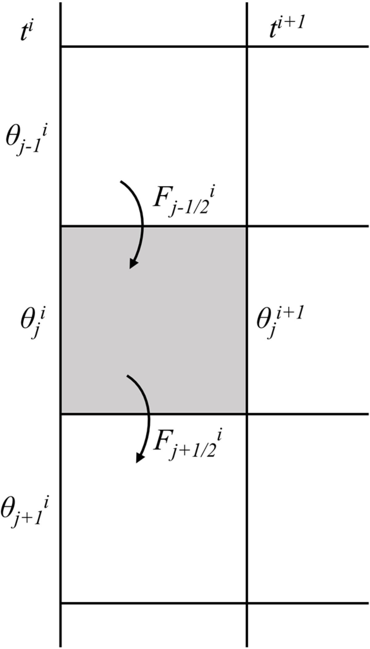
2.2.2. Explicit Formulation

As said previously, together with robustness and mass conservation, other required characteristics for the proposed model are computational efficiency and ease of implementation. The Richards equation can be solved by using explicit or implicit formulation in time. The implicit formulation leads to an unconditionally stable scheme, but it is computationally demanding and hard to implement, because of the need to solve, at each time step, a nonlinear equation through iterative procedures like the Picard, Newton-Raphson, or Secant methods.

On the other hand, the explicit formulation is easy to implement, computationally efficient and leads to a conservative scheme, while being conditionally stable. For these reasons, the explicit formulation in time was chosen and used.

In one space dimension, the Finite Volume Method is based on subdividing the domain into finite grid cells and on approximation of the flux on the boundary of these cells (Figure 2).

Figure 2. Illustration of the Finite Volume Scheme for updating the cell values by the boundary fluxes.

Figure 2. Illustration of the Finite Volume Scheme for updating the cell values by the boundary fluxes.

The general scheme for the Finite Volume Method is explained by the following equation:

$${\text{θ}}_j^{i+1}={\text{θ}}_j^i-\frac{\text{Δ}t}{\text{Δ}z}\left(F_{j+1/2}^i-F_{j-1/2}^i\right)$$

(22)

where Fⁱ_j+1/2 is a numerical approximation of the flux along z = z_j+1/2. A fully discrete method is obtained by approximating the average flux based on the θⁱ values of the cells that are adjacent to the boundary in question. In the case of the upwind method, the flux through the top edge of the cell is entirely determined by the value θⁱ_j−1 in the cell above. The numerical flux for the upwind method is written as:

$$F_{j-1/2}^i=Q({\text{θ}}_{j-1}^i)$$

(23)

A 1D explicit formulation is obtained by using a forward Euler scheme in time and the upwind discretization in space, with a uniform grid spacing:

$${\text{θ}}_j^{i+1}={\text{θ}}_j^i-\frac{\text{Δ}t}{\text{Δ}z}\left[Q_j^i-Q_{j-1}^i\right]$$

(24)

where Q represents the numerical flux:

$$Q=\{\begin{array}{c}{Q}_j^i=-K({\text{θ}}_j^i)\left(\frac{\partial \text{ψ}({\text{θ}}_j^i)}{\partial z}-1\right)\\ Q_{j-1}^i=-K({\text{θ}}_{j-1}^i)\left(\frac{\partial \text{ψ}({\text{θ}}_{j-1}^i)}{\partial z}-1\right)\end{array}$$

(25)

The 1D explicit finite-volume formulation becomes:

$${\text{θ}}_j^{i+1}={\text{θ}}_j^i-\frac{\text{Δ}t}{\text{Δ}z}\left\{K({\text{θ}}_{j-1}^i)\left[\frac{{\text{ψ}}_j^i-{\text{ψ}}_{j-1}^i}{\text{Δ}z}-1\right]-K({\text{θ}}_j^i)\left[\frac{{\text{ψ}}_{j+1}^i-{\text{ψ}}_j^i}{\text{Δ}z}-1\right]\right\}$$

(26)

As stated earlier, the explicit formulation is conditionally stable, and for that reason, it imposes some restrictions on time step selection. A necessary, but not sufficient, condition for the stability of a finite volume or finite difference scheme for the resolution of a partial differential equation (PDE) is that the numerical domain of dependence contains the mathematical domain of dependence. This requirement is known as the Courant-Friedrichs-Levy or CFL condition. The Courant number for the Richards equation can be written as [25]:

$$CFL=\frac{\left|v\right|\text{Δ}t}{\text{Δ}z}=\frac{\partial K}{\partial \text{θ}}\frac{\text{Δ}t}{\text{Δ}z}$$

(27)

where v is the soil water velocity (LT⁻¹). The Courant number reflects the importance of the convective flux in the unsaturated flow.

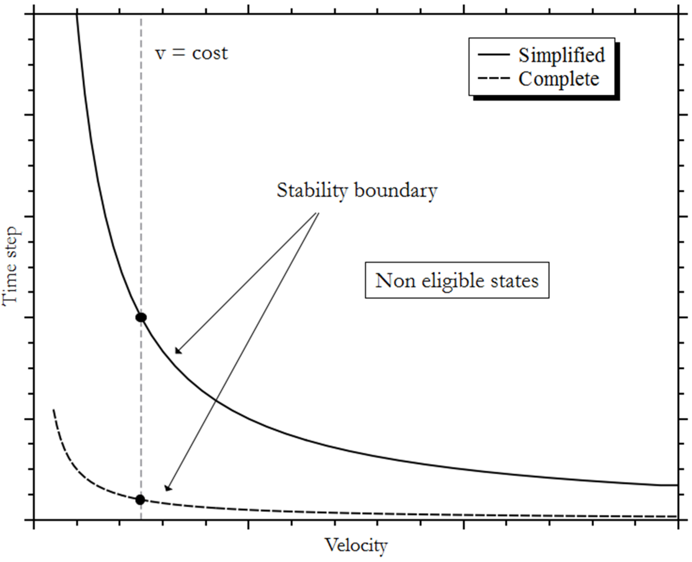
The stability condition for the explicit upwind scheme can be written as:

$$\frac{2D\text{Δ}t}{\text{Δ}{z}^2}+\frac{\left|v\right|\text{Δ}t}{\text{Δ}z}\le 1$$

(28)

where v is the velocity, D is the diffusivity, Δt is the time step and Δz is the mesh size. This formulation includes the diffusion number condition.

2.3. Green Roof Substrate

As stated in the introduction, the substrate is one of the most important elements of a green roof; the characteristics of this element strongly influence the hydraulic behaviour of the green roof.

Typical green roof growing media are composed of 80%–90% light-weight aggregate (LWA) and 10%–20% fine material [26]. LWA provides pore space for air and water and ensures rapid drainage. However, the low organic content and the coarse texture imply that key functions for plant growth must be supplemented, e.g., by cation exchange capacity (CEC) for nutrient retention and chemical buffering and moisture storage and supply. The LWA mainly consists of expanded clay, expanded shale, expanded slate, or similar material. Aggregates are usually mixed with sand and organic matter, in order to provide an adequate portion of fine particulate matter supporting the plants. Recycled clay bricks and crushed concrete may be used as aggregate components. They are not lightweight, but their coarse particles possess high permeability. Extensive green roof substrates are typically 5%–20% organic material. The Forschungsgesellschaft Landschaftsentwiklung Landschaftsbau (FLL) guidelines [26] recommend a maximum organic content of 65 g/L. A high proportion of organic matter increases water retention capacity and may benefit plant growth, but decreases the GR permeability. Maintaining high permeability in the porous matrix is fundamental for avoiding ponding and surface runoff.

The FLL guidelines further indicates that the combined silt and clay content (d < 0.063 mm) of an extensive green roof should not exceed 15% by mass. Excessive fine particles will reduce substrate permeability and increase weight.

In intensive green roof substrates, the content of silt and clay should not exceed 20%, with an organic content <12%.

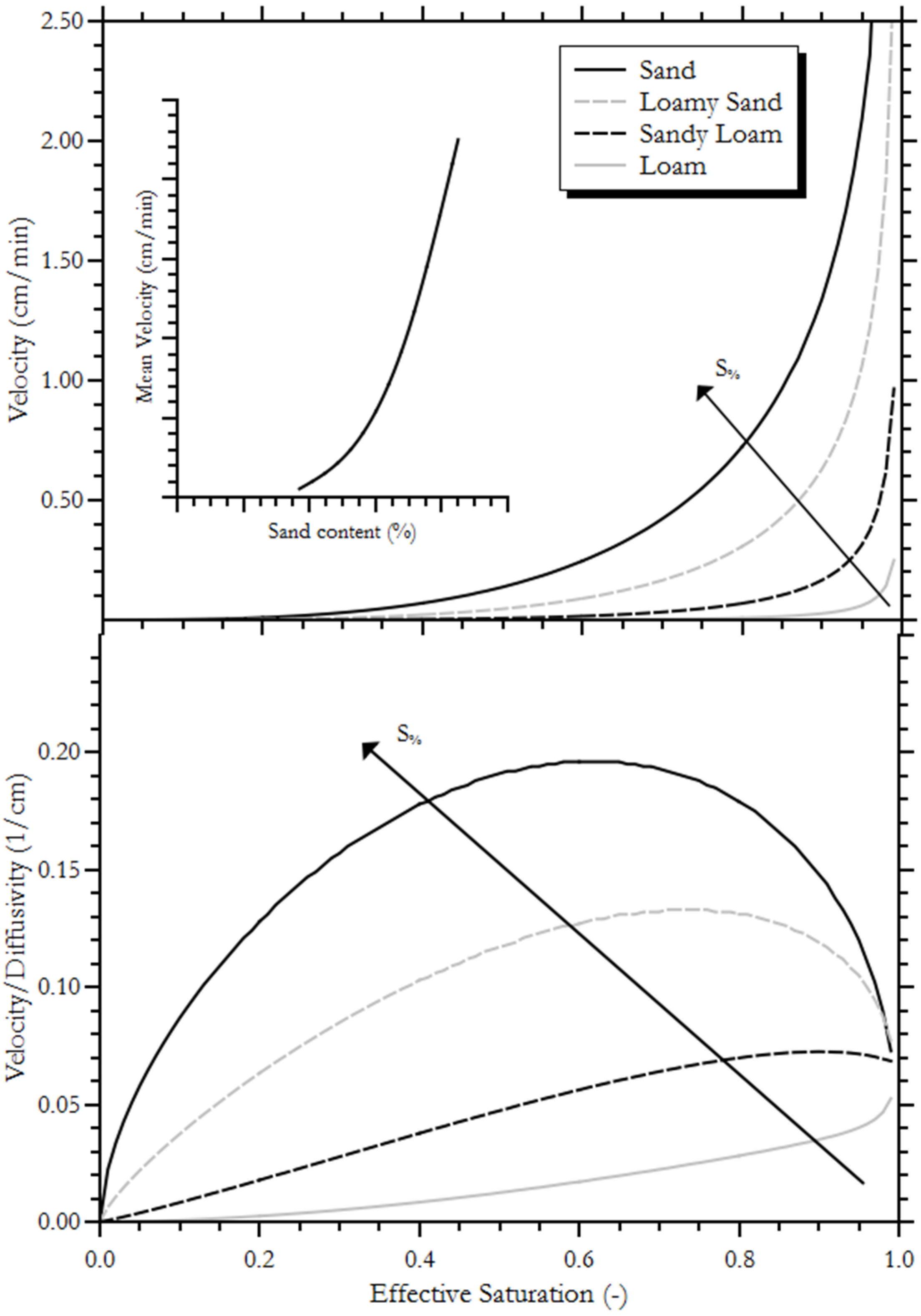
In summary, a coarse porous matrix, with a low organic content and high permeability, is characteristic for GR substrates. These features influence the hydraulic behaviour of GRs, especially in terms of the wetting front velocity and characteristics of the unsaturated flow. As pointed out in the literature [25], velocities and Peclet numbers are higher for coarse soils, and can vary by several orders of magnitude over the saturation field.

It is evident from Figure 3 that water velocity is directly related to sand content, and in particular, it increases exponentially as the soil becomes coarser. On the other hand, the velocity/diffusivity ratio describes the nature of the unsaturated flow. The definition of such an index is suggested by the similarity between the Richards equation and the advection-dispersion equation. High values of this ratio indicate that the flow is mainly advective, while low values are associated mostly with a diffusive flow characterized by low velocities.

In view of the characteristics of GR substrates, and according to the preceding discussion, the flow in the porous matrix of green roofs must be strongly unsaturated and mainly advective, with high velocities.

Figure 3. Water velocity and ratio velocity/diffusivity for four selected typical soils.

Figure 3. Water velocity and ratio velocity/diffusivity for four selected typical soils.

2.4. Simplified Formulation

From a computational point of view, within the limits of the stability condition, the upwind discretization guarantees the robustness and monotonicity of the numerical scheme, but introduces false numerical diffusion into the solution. To attenuate this diffusion, it is necessary to use a very fine mesh. However, this condition for an explicit scheme imposes the requirement of selecting very small time steps, in order to satisfy the stability condition [27], and results in high computational requirements. On the other hand, green roof substrates are characterized by strongly unsaturated flows with high velocities, and under such conditions, the diffusive term becomes less important. From these considerations arises the idea of proposing a simplified formulation of the Richards equation, in which the diffusive term is neglected. The Darcy equations becomes:

$$q=K(\text{θ})$$

(29)

By substituting this relation into the continuity Equation (2), the following equation is obtained:

$$\frac{\partial \text{θ}}{\partial t}+\nabla K(\text{θ})=0$$

(30)

The governing equation then becomes a hyperbolic PDE, in which the time variation of the volumetric water content depends only on the divergence of the unsaturated hydraulic conductivity.

The 1D explicit finite formulation, using the upwind discretization in space, can be written as:

$${\text{θ}}_j^{i+1}={\text{θ}}_j^i-\frac{\text{Δ}t}{\text{Δ}z}\left[Q_j^i-Q_{j-1}^i\right]$$

(31)

where Q represents the numerical flux, defined as:

$$Q=\{\begin{array}{c}{Q}_j^i=K({\text{θ}}_j^i)\\ Q_{j-1}^i=K({\text{θ}}_{j-1}^i)\end{array}$$

(32)

The 1D explicit finite-volume formulation becomes:

$${\text{θ}}_j^{i+1}={\text{θ}}_j^i-\frac{\text{Δ}t}{\text{Δ}z}\left[K({\text{θ}}_j^i)-K({\text{θ}}_{j-1}^i)\right]$$

(33)

Obviously, the neglect of the diffusive term in the mathematical formulation introduces an error into the solution, even for highly permeable soils where the flow is predominantly controlled by gravity, as is the case in the green roof substrates. However, this effect can be offset by the numerical diffusion introduced by the upwind scheme by appropriately selecting the mesh size in the discretization of the domain.

The numerical diffusion (ND) introduced by the upwind scheme arises from a first-order approximation of the spatial derivative ∂θ/∂z, this is evident if we examine the Taylor series expansion:

$$\text{θ}(z_{j+1})=\text{θ}(z_j)+{\frac{\partial \text{θ}}{\partial z}|}_{z_j}(\text{Δ}z)+\frac{1}{2}{\frac{{\partial }^2\text{θ}}{\partial z^2}|}_{z_j}{(\text{Δ}z)}^2+\text{ (Higher order terms)}$$

(34)

The first derivative can be written as:

$$\frac{\partial \text{θ}}{\partial z}=\frac{\text{θ}(z_j)-\text{θ}(z_{j-1})}{\text{Δ}z}-\frac{1}{2}\frac{{\partial }^2\text{θ}}{\partial z^2}(\text{Δ}z)-\frac{1}{\text{Δ}z}\text{ (Higher order terms)}$$

(35)

The Equation (30) can be written as:

$$\frac{\partial \text{θ}}{\partial t}+\frac{\partial K(\text{θ})}{\partial \text{θ}}\frac{\partial \text{θ}}{\partial z}=0$$

(36)

where the derivative ∂K(θ)/∂z is the soil water velocity v. By substituting Equation (35) into Equation (36) we obtain:

$$\frac{\partial \text{θ}}{\partial t}+v\left(\frac{\text{θ}(z_j)-\text{θ}(z_{j-1})}{\text{Δ}z}\right)=v\left(\frac{1}{2}\frac{{\partial }^2\text{θ}}{\partial z^2}(\text{Δ}z)+\frac{1}{\text{Δ}z}\text{ (Higher order terms)}\right)$$

(37)

The higher order terms are much smaller than the second derivative, so they can be ignored. The Equation (37) becomes:

$$\frac{\partial \text{θ}}{\partial t}+v\left(\frac{\text{θ}(z_j)-\text{θ}(z_{j-1})}{\text{Δ}z}\right)=ND\frac{{\partial }^2\text{θ}}{\partial z^2}$$

(38)

where ND is the numerical diffusion defined as in Equation (21).

In order to produce accurate results, the numerical diffusion (ND) introduced by the upwind scheme must compensate for the diffusive term neglected in Equation (30). Equation (6) can be written as:

$$\frac{\partial \text{θ}}{\partial t}-\frac{\partial }{\partial z}(D(\text{θ})\frac{\partial \text{θ}}{\partial z})+\frac{\partial K(\text{θ})}{\partial z}=0$$

(39)

$$\frac{\partial \text{θ}}{\partial t}-\frac{\partial D(\text{θ})}{\partial z}\frac{\partial \text{θ}}{\partial z}-D(\text{θ})\frac{{\partial }^2\text{θ}}{\partial z^2}+\frac{\partial K(\text{θ})}{\partial \text{θ}}\frac{\partial \text{θ}}{\partial z}=0$$

(40)

$$\frac{\partial \text{θ}}{\partial t}+\frac{\partial K(\text{θ})}{\partial \text{θ}}\frac{\partial \text{θ}}{\partial z}=\frac{\partial D(\text{θ})}{\partial z}\frac{\partial \text{θ}}{\partial z}+D(\text{θ})\frac{{\partial }^2\text{θ}}{\partial z^2}$$

(41)

Equation (41) is similar to Equation (38). Combining these two equations leads to:

$$ND\frac{{\partial }^2\text{θ}}{\partial z^2}=\frac{\partial D(\text{θ})}{\partial z}\frac{\partial \text{θ}}{\partial z}+D(\text{θ})\frac{{\partial }^2\text{θ}}{\partial z^2}$$

(42)

$$ND=D(\text{θ})+\frac{\frac{\partial D(\text{θ})}{\partial z}\cdot \frac{\partial \text{θ}}{\partial z}}{\frac{{\partial }^2\text{θ}}{\partial z^2}}$$

(43)

This relationship regulates the amount of numerical diffusion that must be introduced in order to compensate for the nonlinear diffusive term ignored in Equation (6). This value cannot be determined a priori due to the variation of θ along z during the simulation. For these reasons, in order to have a first approximation of the value of ND, some assumptions must be made.

A first approximation of ND can be obtained by equating the numerical diffusion to the soil water diffusivity. However, this type of approximation leads to poor accuracy due to the neglect of the effect of second term on the right side of Equation (43). This term is directly related to the first and second derivatives of the soil moisture profile and cannot be determined a priori, without some simplifying assumptions.

In this research, the mesh size was determined by assuming:

$$ND=\frac{D}{2}$$

(44)

Combining Equations (44) and (21) leads to:

$$\text{Δ}z=\frac{D}{v}$$

(45)

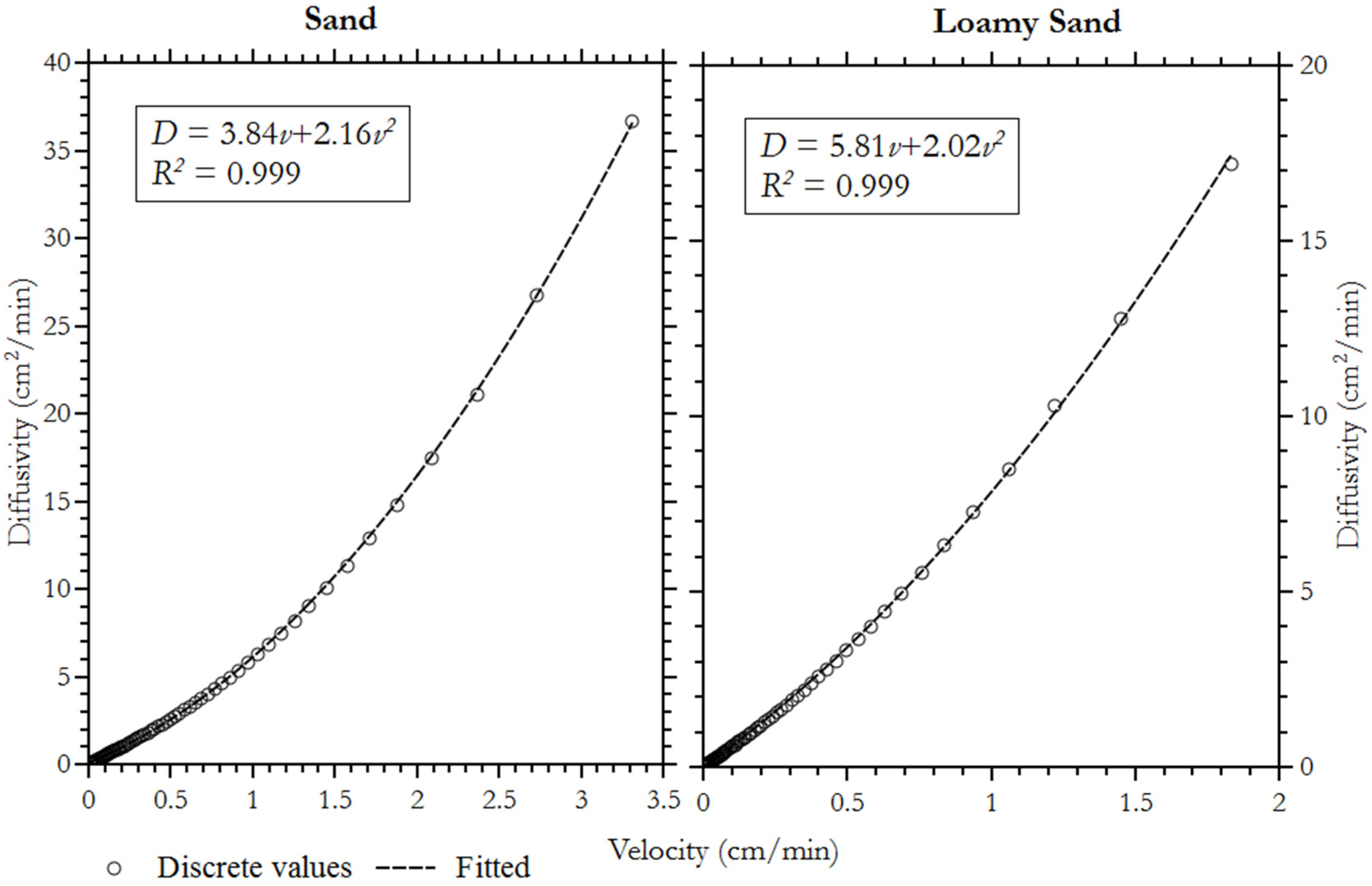
The mesh size Δz, defined in Equation (45), is the function of two variables: soil water diffusivity D and soil water velocity v. In order to simplify the above equation, we tried to find a relationship between D and v. In Figure 4, a scatter plot of the discrete values of the two variables v and D is presented.

Figure 4. Parabolic relation between velocity and diffusivity.

Figure 4. Parabolic relation between velocity and diffusivity.

We performed a polynomial regression on the discrete values using the algorithm from Levenberg-Marquadt. As shown in Figure 4, the soil water diffusivity is related to the water velocity by a parabolic relationship, which can be written as:

$$D=\text{λ}\cdot v+\text{ω}\cdot v^2$$

(46)

where λ and ω are two parameters that depend on the soil type. The Pearson coefficient R² for the two-polynomial regression is very high.

Combining Equation (46) with Equation (45) leads to:

$$\text{Δ}z=\text{λ}+\text{ω}\cdot v$$

(47)

For a given velocity value, it is possible to determine the mesh size that ensures a consistent numerical diffusion.

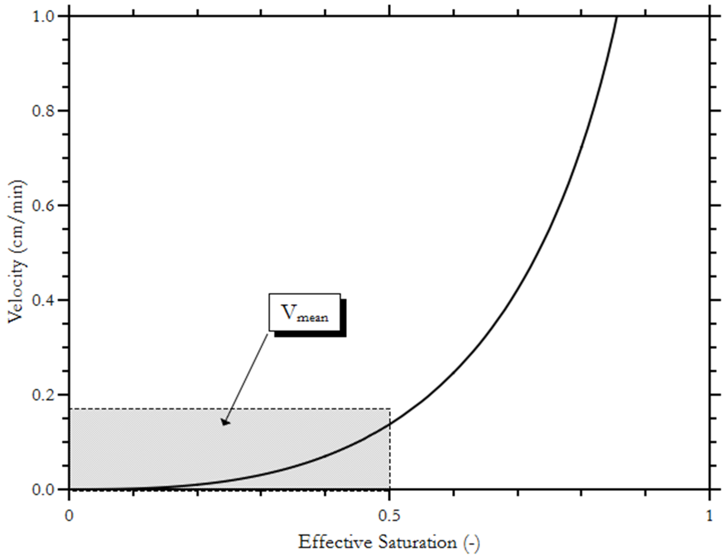
During the rainfall event, the velocity of the wetting front in the substrate is highly variable, depending on the soil characteristics. Green roof substrates are characterized by high permeability that implies fast drainage and low moisture content of the substrate during rainfall events [28]. As already stated in the literature, the saturation degree for green roof substrates does not exceed 50% [29,30,31]. For these reasons, the mesh size Δz is computed by assuming that the velocity in the green roof substrate varies between 0% and 50%, and calculating a mean value in this range (Figure 5). By substituting this value into Equation (47), it is possible to obtain the value of the mesh size Δz.

Figure 5. Computation of the velocity value for the determination of the mesh size as indicated in Equation (47).

Figure 5. Computation of the velocity value for the determination of the mesh size as indicated in Equation (47).

2.5. Model Performance Evaluation

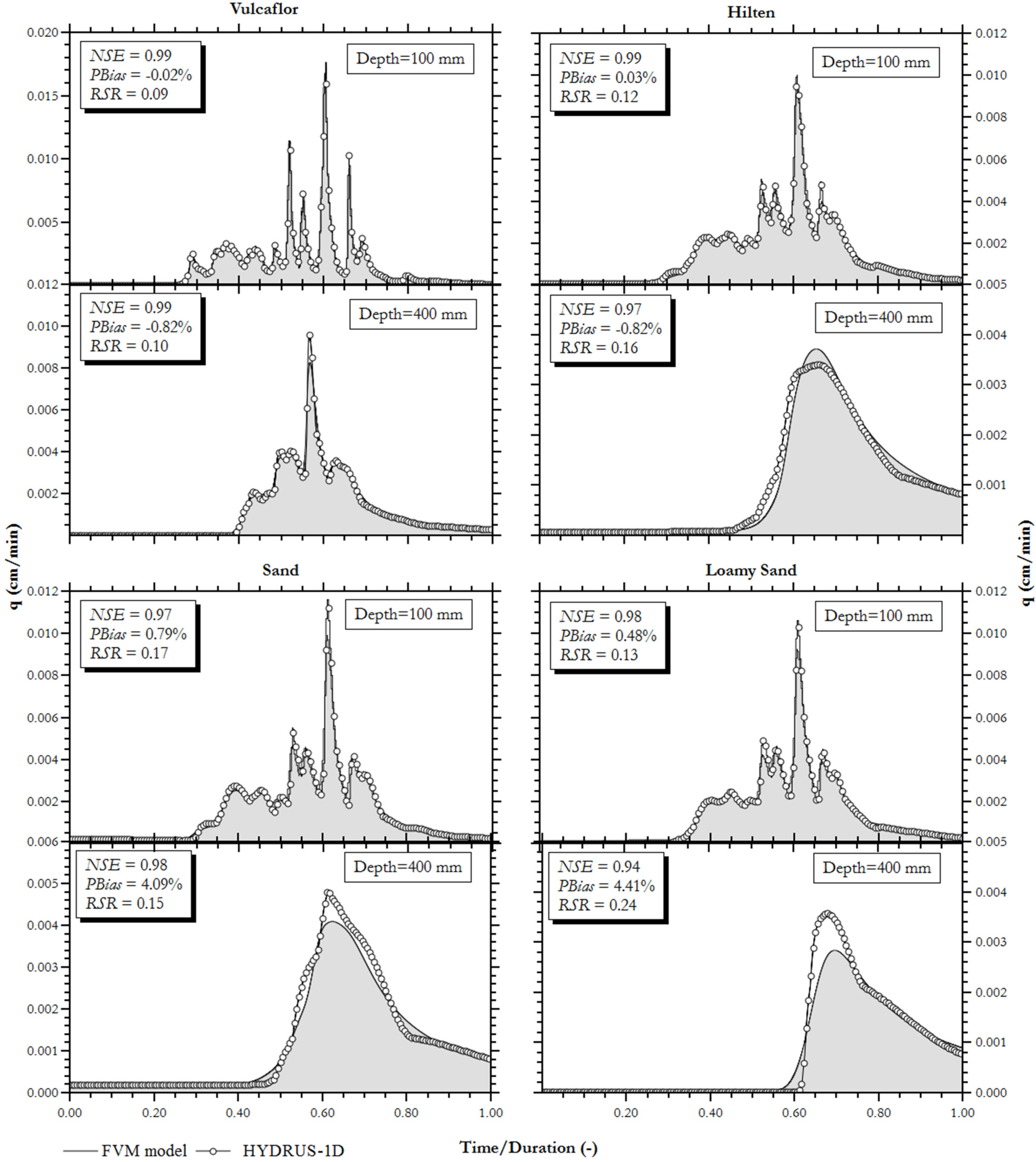
The proposed Finite Volume solution was compared to numerical simulations performed using HYDRUS-1D [32]. HYDRUS-1D is a finite-element software that numerically solves the Richards equation for saturated-unsaturated water flows and it is one of the best documented and most widely used codes. In view of its reliability, HYDRUS-1D has been used in the literature as a benchmark for the validation of different alternative models [11,33], and therefore, it was used in this study as well for comparing the outflow rates from the green roof substrate. The outflow is one of the most important hydraulic characteristics in the analysis of a green roof exposed to rainfall; it provides information on the retention and peak attenuation capacity of the green roof, and for these reasons, accurate modelling of the GR outflow is particularly needed.

In order to perform the comparison between the two models, boundary conditions must be defined. Boundary conditions of interest for 1D vertical flow are only the top and bottom boundaries. In this study, two Neumann boundary conditions have been applied.

Neumann boundary conditions specify the value of the flux in the direction normal to the boundary considered. For the top boundary, the infiltration process has been simulated by imposing a Neumann condition, specifying the value of the flux.

Precisely, when dealing with infiltration fluxes at the soil surface, the most widely used boundary condition is the soil-atmosphere interface condition, which permits switching between the Neumann and Dirichlet boundary conditions depending on the state of the soil surface. During infiltration a Neumann condition is applied. If the applied flux is larger than the saturated hydraulic conductivity, then positive pressures appear at the surface, which corresponds to the formation of ponding on the soil surface. At this point the boundary condition switches to the Dirichlet boundary condition. However, as stated previously, green roof substrates are designed to avoid the formation of ponding on the surface, which is why the Neumann boundary condition has been implemented.

For the bottom boundary condition, a free drainage condition has been used. The free drainage condition represents vertical flow of water through the bottom of the soil towards a distant groundwater table. This condition is of the Neumann type.

The same boundary conditions have been selected in HYDRUS. In particular, an atmospheric boundary condition with surface runoff for the top boundary, and a free drainage condition for the bottom.

For a quantitative assessment of the model performance, several statistical indices were found in the literature. One of the most important features of a numerical scheme to be evaluated is its ability to conserve mass over the entire domain. Such conservation is an essential condition for a numerical scheme. To measure the ability of the model to conserve mass, the mass balance ratio proposed by Celia [10] can be used:

$$MBR=\frac{\text{total additional mass in the domain}}{\text{total net flux in the domain}}=\frac{{\displaystyle \sum _{j=1}^N({\text{θ}}_n-{\text{θ}}_0)\cdot \text{Δ}z}}{{\displaystyle \sum _{i=1}^T(q_{in}-q_{ef})\cdot \text{Δ}t}}$$

(48)

where θ₀ is the initial mass in the domain (L³L⁻³), θ_n is the final mass (L³L⁻³), q_in is the influent flow in the domain (LT⁻¹), q_ef is the effluent (LT⁻¹), Δz is the mesh size (L), Δt is the time step (T), N is the number of finite volume elements of the domain, and i is the time index.

The mass balance ratio is a necessary, but not sufficient, condition for acceptability of a numerical model. In order to compare the proposed model with HYDRUS-1D, three statistical indices were selected.

The Nash-Sutcliffe Efficiency (NSE) is one of the most widely used indices for characterizing the overall fit of hydrographs [34]. The NSE is computed as follows:

$$NSE=1-\left[\frac{{\displaystyle \sum _{i=1}^T{(Q_i^{obs}-Q_i^{\text{mod}})}^2}}{{\displaystyle \sum _{i=1}^T{(Q_i^{obs}-Q_{mean}^{obs})}^2}}\right]$$

(49)

where $Q_i^{obs}$ is the ith reference value, $Q_i^{mod}$ is the ith simulated value, and Q_mean^obs is the mean value of observed data. NSE coefficient ranges between −∞ and 1.0, in the case of a perfect agreement; generally, values 0 and 1.0 are considered acceptable.

Percent bias (PBias) measures the average tendency of the model to overestimate or underestimate the counterpart [35]. Small values indicate good performance from the model, negative values indicate overestimation, and positive values indicate underestimation. PBias is calculated as follows:

$$PBias(\%)=\frac{{\displaystyle \sum _{i=1}^T(Q_i^{obs}-Q_i^{sim})}}{{\displaystyle \sum _{i=1}^T{Q}_i^{obs}}}\cdot 100$$

(50)

PBias was selected for its ability to clearly indicate poor model performance.

Various error indices are commonly used for model evaluations. The Mean Absolute Error (MAE), Mean Square Error (MSE) and Root Mean Square Error (RMSE) are most widely used. The smaller the error value, the better the model performance, but only Singh and Bengtsson [34] have published guidelines, based on the observations of standard deviations, on what magnitude of small RMSEs is acceptable. Following this guideline, the RMSE-observations/standard deviation ratio (RSR) was used. The RSR is calculated as the ratio of the RMSE and the standard deviation of reference data, as shown in Equation (34):

$$RSR=\frac{RMSE}{STDE{V}_{obs}}=\frac{\left[\sqrt{{\displaystyle \sum _{i=1}^T{(Q_i^{obs}-Q_i^{sim})}^2}}\right]}{\left[\sqrt{{\displaystyle \sum _{i=1}^T{(Q_i^{obs}-Q_{mean}^{obs})}^2}}\right]}$$

(51)

The RSR varies from the optimal value of 0 to large positive values.

The proposed model has been implemented in the Python programming language.

3. Results and Discussion

In this research, four types of soils covering a wide range of plausible green roof substrates were considered: sand, loamy sand, Vulcaflor and Hilten soil [36]. Loamy sand is a soil material that contains between 70% and 90% sand, and the remaining parts are silts and clay [37]. Sand is a soil material that contains 85% or more sand; the percentage of silt plus 1.5 times the percentage of clay does not exceed 15%. In addition to these two types of soils, two other typical soils for the GR substrates were identified in the literature. Vulcaflor soil was reported in [38]; it is a mixture of volcanic material and organic matter (16%). The PSD curve for Vulcaflor indicates that it can be classified as a fine gravel soil according to the Unified Soil Classification System. In [36] an engineered green roof substrate was analyzed using a pressurized temple cell in order to identify its hydraulic properties and the soil water retention curve. Hilten soil is composed of 80% expanded slate and 20% organic matter. Water content at 33 kPa and 1500 kPa determines the field capacity and the wilting point, respectively, and were found to be 0.11 m³m⁻³ and 0.08 m³m⁻³.

The Mualem-van Genuchten parameters for Hilten soil were determined by using the Rosetta software [39], which estimates the unsaturated hydraulic properties from the soil texture data, bulk density, field capacity and the wilting point. The Rosetta model is based on a pedotransfer function (PTF) and translates basic soil data into soil hydraulic properties.

The Mualem-van Genuchten parameters for the selected soils are listed in Table 1:

Table 1. Mualem-van Genuchten parameters for the selected soils.

Substrate Soils	θr (-)	θs (-)	α (1/cm)	n	K0 (cm/min)
Vulcaflor	0.165	0.400	0.124	2.280	4.800
Hilten	0.045	0.570	0.065	2.320	1.720
Sand	0.045	0.430	0.145	2.680	0.495
Loamy sand	0.065	0.41	0.075	1.89	0.074

Notes: θ_r is the soil residual water content; θ_s is the saturated soil water content; α and n are two characteristic parameters of the MG model; and K₀ is the matching point at saturation.

Table 1. Mualem-van Genuchten parameters for the selected soils.

Substrate Soils	θr (-)	θs (-)	α (1/cm)	n	K0 (cm/min)
Vulcaflor	0.165	0.400	0.124	2.280	4.800
Hilten	0.045	0.570	0.065	2.320	1.720
Sand	0.045	0.430	0.145	2.680	0.495
Loamy sand	0.065	0.41	0.075	1.89	0.074

Notes: θ_r is the soil residual water content; θ_s is the saturated soil water content; α and n are two characteristic parameters of the MG model; and K₀ is the matching point at saturation.

The soil water retention curves computed using the MG model are displayed in Figure 6:

Figure 6. Retention curves for selected soils.

Figure 6. Retention curves for selected soils.

The initial moisture condition was assumed to be constant over the whole soil profile, and specifically, it was set equal to the field capacity value. The field capacity for each soil was determined using the relationship from Twarakavi [40] given a negligible drainage flux of 0.01 cm/day:

$${\text{Θ}}_{fc}=n^{-0.60(2+{\text{log}}_{10}(K_s))}$$

(52)

The values of the field capacity for all soils are listed in Table 2:

Table 2. Field capacity value of selected soils.

Substrate Soils	Θfc (-)	θfc (-)
Vulcaflor	0.056	0.178
Hilten	0.066	0.079
Sand	0.057	0.067
Loamy Sand	0.106	0.094

Notes: Θ_fc is the field capacity value in terms of effective saturation; θ_fc is the field capacity in terms of volumetric water content.

Table 2. Field capacity value of selected soils.

Substrate Soils	Θfc (-)	θfc (-)
Vulcaflor	0.056	0.178
Hilten	0.066	0.079
Sand	0.057	0.067
Loamy Sand	0.106	0.094

Notes: Θ_fc is the field capacity value in terms of effective saturation; θ_fc is the field capacity in terms of volumetric water content.

Ten measured rainfall events were selected for the validation of the proposed model. The rainfall data were collected by a tipping-bucket rain gauge installed at the University of Calabria in Rende. The rain gauge has a resolution of 0.2 mm and was calibrated in the laboratory according to the World Meteorological Organization’s specifications [41].

The characteristics of the selected rainfall events are listed in Table 3:

Table 3. Hydrologic characteristics of the selected rainfall events.

Rainfall Event	h (mm)	imax (mm/h)	D (min)
11 November 2013 00:27	64.2	96.0	1599
22 November 2013 23:31	69.0	60.0	3116
29 November 2013 22:19	48.0	24.0	3301
26 December 2013 09:58	26.2	12.0	1648
20 January 2014 17:39	48.2	48.0	2710
31 January 2014 18:54	33.8	24.0	2448
02 February 2014 19:43	27.8	24.0	1944
11 February 2014 22:58	29.6	24.0	2039
23 March 2014 21:55	40.4	36.0	2357
27 March 2014 02:27	31.8	36.0	2507

Notes: h: rainfall depth of the rainfall event (mm); i_max: max intensity during the rainfall event (mm/h); D: duration of the event (min).

Table 3. Hydrologic characteristics of the selected rainfall events.

Rainfall Event	h (mm)	imax (mm/h)	D (min)
11 November 2013 00:27	64.2	96.0	1599
22 November 2013 23:31	69.0	60.0	3116
29 November 2013 22:19	48.0	24.0	3301
26 December 2013 09:58	26.2	12.0	1648
20 January 2014 17:39	48.2	48.0	2710
31 January 2014 18:54	33.8	24.0	2448
02 February 2014 19:43	27.8	24.0	1944
11 February 2014 22:58	29.6	24.0	2039
23 March 2014 21:55	40.4	36.0	2357
27 March 2014 02:27	31.8	36.0	2507

Notes: h: rainfall depth of the rainfall event (mm); i_max: max intensity during the rainfall event (mm/h); D: duration of the event (min).

Numerical simulations were performed for two different depths of the substrate: s = 100 mm, which is a typical value for extensive green roofs, and s = 400 mm, which is typical for intensive green roofs.

3.1. Results

The numerical simulations were conducted by choosing a time step of 6 s and computing the mesh size from Equation (47). Computational parameters are shown in Table 4 for the two depths studied.

Table 4. Simulation parameters.

Substrate Soils	λ (-)	ω (-)	Vm (cm/min)	Δz (cm)	N100 (-)	N400 (-)
Vulcaflor	10.3	0.196	0.218	10.3	1	4
Hilten	8.36	0.52	0.084	8.4	2	5
Sand	3.84	2.16	0.036	3.9	3	10
Loamy sand	5.81	2.02	0.011	4.7	2	7

Notes: λ and ω are the two parameters featured in Equation (29); V_m is the mean value of the velocity computed by assuming that the saturation range does not exceed 50%; Δz is the mesh size calculated by using Equation (30); N₁₀₀ and N₄₀₀ are the numbers of subdivision elements for the two selected substrate depths.

Table 4. Simulation parameters.

Substrate Soils	λ (-)	ω (-)	Vm (cm/min)	Δz (cm)	N100 (-)	N400 (-)
Vulcaflor	10.3	0.196	0.218	10.3	1	4
Hilten	8.36	0.52	0.084	8.4	2	5
Sand	3.84	2.16	0.036	3.9	3	10
Loamy sand	5.81	2.02	0.011	4.7	2	7

Notes: λ and ω are the two parameters featured in Equation (29); V_m is the mean value of the velocity computed by assuming that the saturation range does not exceed 50%; Δz is the mesh size calculated by using Equation (30); N₁₀₀ and N₄₀₀ are the numbers of subdivision elements for the two selected substrate depths.

Results of the numerical simulations for the two depths considered are listed in Table 5. In particular, the mean value and the standard deviation for each index are reported.

Table 5. Statistical evaluation of comparisons between the proposed FV model and HYDRUS-1D.

Soil	NSE100 (-)	NSE400 (-)	PBias100 (%)	PBias400 (%)	RSR100 (-)	RSR400 (-)
Vulcaflor	0.95 ± 0.04	0.99 ± 0.01	0.45 ± 0.39	−1.17 ± 0.45	0.23 ± 0.07	0.10 ± 0.01
Hilten	0.97 ± 0.01	0.89 ± 0.06	−0.03 ± 0.24	−1.96 ± 0.69	0.16 ± 0.03	0.33 ± 0.09
Sand	0.98 ± 0.01	0.95 ± 0.03	0.52 ± 0.18	1.74 ± 0.53	0.12 ± 0.03	0.23 ± 0.06
Loamy sand	0.98 ± 0.01	0.95 ± 0.02	0.78 ± 0.28	2.17 ± 1.09	0.13 ± 0.03	0.22 ± 0.06

Notes: NSE is the Nash-Sutcliffe efficiency index; PBias is the Percent Bias index; RSR is the RMSE- observations/standard deviation ratio. Each index is calculated for the two depths considered.

Table 5. Statistical evaluation of comparisons between the proposed FV model and HYDRUS-1D.

Soil	NSE100 (-)	NSE400 (-)	PBias100 (%)	PBias400 (%)	RSR100 (-)	RSR400 (-)
Vulcaflor	0.95 ± 0.04	0.99 ± 0.01	0.45 ± 0.39	−1.17 ± 0.45	0.23 ± 0.07	0.10 ± 0.01
Hilten	0.97 ± 0.01	0.89 ± 0.06	−0.03 ± 0.24	−1.96 ± 0.69	0.16 ± 0.03	0.33 ± 0.09
Sand	0.98 ± 0.01	0.95 ± 0.03	0.52 ± 0.18	1.74 ± 0.53	0.12 ± 0.03	0.23 ± 0.06
Loamy sand	0.98 ± 0.01	0.95 ± 0.02	0.78 ± 0.28	2.17 ± 1.09	0.13 ± 0.03	0.22 ± 0.06

Notes: NSE is the Nash-Sutcliffe efficiency index; PBias is the Percent Bias index; RSR is the RMSE- observations/standard deviation ratio. Each index is calculated for the two depths considered.

Results confirm the ability of the proposed model to correctly describe the unsaturated flow in both substrates. The excellent agreement between the proposed model and HYDRUS-1D (Figure 7) is confirmed by the values of NSE and RSR. Low values of the PBias indicate that the proposed model does not overestimate or underestimate the outflow, except for small quantities. This is confirmed by the optimal value of MBR being always equal to 1, which indicates a very good conservation of mass.

Figure 7. Graphical and statistical evaluations of comparing the proposed model soil outflow rates to those produced by Hydrus-1D, for the event of 29 November 2013 22:19:00 and the Vulcaflor soil.

Figure 7. Graphical and statistical evaluations of comparing the proposed model soil outflow rates to those produced by Hydrus-1D, for the event of 29 November 2013 22:19:00 and the Vulcaflor soil.

As stated in the previous section, another desired requirement for the proposed model is the computational efficiency, together with conservation of mass. Within the limits imposed by the stability condition, conservation is guaranteed by the monotonicity of the upwind discretization. On the other hand, computational efficiency is directly related to the time step and mesh size.

The main advantage of the simplified formulation over the complete explicit formulation, explained in Section 2.2.2, is the assurance of accurate numerical simulations with reduced computational requirements. The complete computational scheme formulation needs a fine mesh subdivision to reduce the effect of the numerical diffusion introduced by the upwind discretization. However, a fine mesh requires very small time steps in order to satisfy the stability condition.

In Figure 8 the stability condition curves for the two formulations are displayed. The two curves are calculated for Vulcaflor soil, and given Δz = 10 cm for the simplified formulation, as shown in Table 4, and Δz = 1 cm for the complete formulation. This value minimizes the effect of the numerical diffusion introduced by the upwind formulation. The curves are calculated on the limit of the stability condition. The time step is then computed as:

$$\text{Δ}t=\frac{\text{Δ}z}{\left|v\right|}$$

(53)

$$\text{Δ}t=\frac{1}{\frac{2D}{\text{Δ}{z}^2}+\frac{\left|v\right|}{\text{Δ}z}}$$

(54)

Equations (53) and (54) represent the stability domains for the two formulations.

Figure 8. The stability condition curves for the two formulations.

Figure 8. The stability condition curves for the two formulations.

As can be seen from Figure 8, the stability domain for the simplified formulation includes a much larger number of eligible states compared to the complete formulation. Therefore, for the same velocity, the complete formulation requires a smaller time step than the simplified one. This results in lower computational demands for the simplified formulation.

In summary, the results confirm the accuracy and computational advantages of the proposed model. One of the most important advantages is the ease of the model’s implementation. The use of an explicit scheme for the resolution of the partial differential equation allows the problem to be linearized and avoids the use of iterative procedures, which are necessary for solving a nonlinear equation.

This aspect, together with the computational efficiency explained earlier, makes the proposed model easy to implement even on spreadsheets. This is crucial for dissemination of physically-based modelling tools that are both accurate and computationally efficient.

Another important aspect is the fact that the proposed model is clearly designed for the analysis of the infiltration process in the substrate of green roofs, which is crucial for describing the hydraulic behaviour of the green roof during rainfall events. Software, such as HYDRUS-1D, although very accurate and comprehensive, is mainly oriented towards numerical analysis in the field of groundwater hydrology. This feature requires experienced users with strong fundamental knowledge and understanding of the modelled processes. This requirement may limit the adoption of physically-based models for analyses of green roofs or LID in general.

4. Conclusions

The main purpose of this research was to develop a physically-based model for hydraulic analysis of green roof substrates. The numerical scheme proposed solves a simplified version of the Richards equation using the Finite Volume Method, which has the advantage of conserving mass both locally and globally.

The proposed model is explicit and therefore easy to implement, and it is based on the upwind discretization in space, which guarantees monotonicity of the solution provided that the stability condition is respected. The numerical scheme is built on the resolution of a modified version of the Richards equation, in which the diffusive term is neglected. The error introduced by this numerical simplification into the solution is compensated for by the effect of the numerical diffusion introduced by the upwind discretization. In this context, a relationship was developed for controlling the numerical diffusion, which is directly related to the mesh size.

The HYDRUS-1D software was used as a benchmark in order to assess the performance of the proposed model. Numerical simulations were conducted for four types of soils typical of green roof substrates and for two different substrate depths. For numerical simulations, ten rainfall events, measured at the University of Calabria, were selected. Roof outflows computed by the two models were compared. The results obtained confirmed the suitability of the proposed model for correctly describing the unsaturated flow in the coarse porous matrix of a green roof. The mean value of the Nash-Sutcliffe index was 0.96, with optimal mass balance ratio, PBias and RSR values.

In addition to accuracy and mass conservation, the proposed model is computationally efficient and offers computational advantages over the complete formulation. This is confirmed by the comparison of the stability curves.

Thus, the proposed model represents a good alternative to the traditional models for analysis of the hydraulic behaviour of green roof substrates. It is physically-based and conserves mass, and furthermore, it is computationally efficient and can be easily implemented in code or a spreadsheet.