Linear Trend Detection in Serially Dependent Hydrometeorological Data Based on a Variance Correction Spearman Rho Method

Abstract

Hydrometeorological data are commonly serially dependent and thereby deviate from the assumption of independence that underlies the Spearman rho trend test. The presence of autocorrelation will influence the significance of observed trends. Specifically, the positive autocorrelation inflates Type І errors, while it deflates the power of trend detection in some cases. To address this issue, we derive a theoretical formula and recommend an appropriate empirical formula to calculate the rho variance of dependent series. The proposed procedure of the variance correction for the Spearman rho method is capable of mitigating the effect of autocorrelation on both, Type І error and power of the test. Similar to the Block Bootstrap method, it has the advantage that it does not require an initial knowledge of the autocorrelation structure or modification of the series. In comparison, the capability of the Pre-Whitening method is sensitive to model misspecification if the series are whitened by a parametric autocorrelation model. The Trend-Free Pre-Whitening method tends to lead to an overestimation of the statistical significance of trends, similar to the original Spearman rho test. The results of the study emphasize the importance of selecting a reliable method for trend detection in serially dependent data.

1. Introduction

In most cases, statistical analyses of monotonic trends in time series require serially independent data. However, the underlying stochastic processes behind the hydrometeorological time series often contain an autocorrelation component, which can strongly affect the statistical significance of the observed trends. The autocorrelation, also known as “serial dependence”, is ubiquitous in hydrometeorological processes (evaporation, stream flow, temperature, rainfall, etc.), especially in data series with sub-annual sampling time scales (i.e., monthly and daily data). Applying a technique that allows for trend detection of serially dependent hydrometeorological series is particularly important when trying to detect weak trends in highly variable time series. Furthermore, trend analyses of serially dependent series often result in an over- or underestimation of the statistical significance of observed trends. This issue was not always sufficiently addressed by studies that are based on the widely used nonparametric rank-based Spearman rho trend test (SR) [1,2,3]. The test is well known for its suitability for data series that have a skew distribution, are censored, or contain missing data. The problem has attracted considerable attention in recent decades, along with an increasing concern related to the impact of intensifying climate change and human activity on the hydrologic cycle [4,5,6,7,8,9,10,11,12].

Several approaches were developed in an attempt to address this problem (Kundzewicz and Robson [13], Khaliq, et al. [14], Sonali and Kumar [15]). Among these efforts, the most widely accepted and applied approaches are Pre-Whitening (PW), Trend-Free Pre-Whitening (TFPW), Block Bootstrap (BBS) and Variance Correction (VC).

The PW approach, proposed by von Storch [16], quantifies the autocorrelation component by the lag-one autoregressive model AR(1). Data are pre-whitened by removing the AR(1) component before applying trend tests. This method is without a doubt meaningful if the series can be represented by an AR(1) process; however, the presence of additional trend components will result in this method falsely removing a portion of a true trend and, by that, reducing the power of the trend test [17]. Moreover, the autocorrelation components are overestimated if the true trend is non-zero. Recognizing these disadvantages, Bayazit and Önöz [18] suggested that PW is not suitable in the case of large sample sizes and strong trends. Hamed [19] improved the PW approach by correcting the bias in the estimation of the lag-one autocorrelation coefficient and carefully selecting the autocorrelation model.

To overcome the adverse interaction between a linear trend component and an AR(1) component, Yue, et al. [20,21] introduced the TFPW approach. The basic idea of this approach is to preserve the true slope of linear trends by removing trend components prior to PW before recombining trend components and trend-free pre-whitened series. Rivard and Vigneault [22] and Blain [23] suggested that TFPW is suitable for trend detection in negative and positive serially dependent data if slopes of trends are estimated properly. However, recent studies provided empirical and theoretical proof that the TFPW is unsuitable to preserve the correct Type І error, which is the only indicator that can be controlled to prevent a false identification of numerous spurious trends. Some variants of the TFPW approach were proposed to achieve more accurate Type І errors, such as the iterative PW procedure [24], the TFPWcu procedure [25], or the Variance Correction Pre-Whitening method (VCPW) [26].

The BBS approach is based on a subdivision of the time series into several blocks. The data are serially dependent in each block but independent among the blocks. Based on this approach, the blocks can be shuffled several times to generate resampled series. Trends are calculated for each resampled series with the goal of deriving an empirical distribution of the test statistic. Subsequently, the test statistic of the original series is compared to the empirical distribution to evaluate the significance of the observed trend. Önöz and Bayazit [27] demonstrated that BBS is a robust choice for detecting trends in serially dependent data. It neither inflates Type І errors nor deflates the power of the test excessively. Alternative bootstrapping approaches are phase randomization [28,29] and sieve bootstrap [30]. All of them have the potential to address the influence of autocorrelation effectively.

Another popular approach to deal with this problem is the Variance Correction (VC) method. It is based on the finding that positive or negative autocorrelation components inflate or deflate the variance of the test statistic, even though they might not alter its asymptotic normality [31]. The VC approach accepts the assumption of serial dependence without prior knowledge of the autocorrelation structure. It is therefore able to handle higher-order dependences than AR(1) [32]. Hamed [33] recently derived a theoretical relationship for computing the variance of the SR statistic for serially dependent data which requires considerable computations. In case of n observations, its calculation requires large numbers of terms which will be of order n⁴. The present study aims at deriving an alternative expression for the same purpose with less computational terms, i.e., ${\mathrm{n}}^2{\left(\mathrm{n}-1\right)}^2/4$. Based on that, the new approach would greatly facilitate multisite trend detection studies. In developing this new method, it is obvious that we need to pay close attention to its capability to correct Type І errors and the power of the SR test.

The main goal of this study is to adapt the SR test to serially dependent data via the VC method, an approach which we name Variance Correction Spearman Rho Trend Test (VC-SR). Our study starts with analyzing the effect of autocorrelation on variance, Type І errors, and power of the original SR test. Subsequently, we develop a theoretical formula and suggest an empirical formula as a practical approximation for computing the variance of the SR statistic that takes into account the effect of autocorrelation. Based on simulation studies, we demonstrate that the proposed procedure is effective in mitigating the effect of autocorrelation on both Type І errors and the power of the test. Finally, we apply the proposed procedure to a real world hydrometeorological time series (potential evapotranspiration) to investigate its applicability and discuss its limitations.

2. The Influence of Autocorrelation on the Original Spearman Rho Trend Test

2.1. The Original Spearman Rho Trend Test

Given a sample data set of observations of the stochastic process ${\mathrm{X}}_{\mathrm{i}}={\mathrm{x}}_1,{\mathrm{x}}_2,\mathrm{...},{\mathrm{x}}_{\mathrm{n}}$, Spearman rho is formulated as:

$$\mathsf{\varrho }=1-\frac{6{\displaystyle \sum _{\mathrm{i}=1}^{\mathrm{n}}{\left[{\mathrm{R}}_{\mathrm{i}}-\mathrm{i}\right]}^2}}{\mathrm{n}\left({\mathrm{n}}^2-1\right)}$$

(1)

where R_i is the rank of the ith observation in the sample of size n, $\mathrm{i}=\text{\hspace{0.17em}}1,2,\mathrm{...},\text{\hspace{0.17em}}\mathrm{n}$ is the chronological order of X_i, ρ denotes the linear correlation between the rank series and the chronological order series. ρ can assume any value between −1 and +1; positive and negative values indicate upward and downward trends in the sample data of X_i, respectively. Correspondingly, ρ = 0 indicates the absence of any trend.

Spearman rho was successfully introduced as a trend test. The null hypothesis H₀ is that X_i is a stationary random process. The basic assumption is that the random variables of X_i at any time are independent and identically distributed. Under this null hypothesis and assumption, the distribution of ρ is asymptotically normal for large n with the mean and variance given by:

$$\mathrm{E}\left(\mathsf{\varrho }\right)=0$$

(2)

$$\mathrm{var}\left(\mathsf{\varrho }\right)=1/\left(\mathrm{n}-1\right)$$

(3)

The standardized SR statistic ${\mathrm{Z}}_{\mathrm{SR}}=\mathsf{\varrho }/\mathrm{var}{\left(\mathsf{\varrho }\right)}^{0.5}$ follows the standard normal distribution ${\mathrm{Z}}_{\mathrm{SR}}~\mathrm{N}\left(0,1\right)$. The significance of a trend can be computed by comparing $\left|{\mathrm{Z}}_{SR}\right|$ with $\left|{\mathrm{Z}}_{\alpha /2}\right|$, which is the absolute value of the $\alpha /2$ quantile of $\mathrm{N}\left(0,1\right)$. If $\left|{\mathrm{Z}}_{\mathrm{SR}}\right|>\left|{\mathrm{Z}}_{\alpha /2}\right|$, the null hypothesis is rejected and the detected trend is statistically significant.

2.2. Rho Variance (Variance of the SR Statistic)

In order to explore how much autocorrelation influences the rho variance, two classic forms, AR(1) and the lag-one moving average model MA(1), which are commonly used to simulate serially dependent hydrometeorological data, are generated by Monte Carlo simulations. The AR(1) model has the form of ${\mathrm{x}}_{\mathrm{i}}={\mathsf{\mu }}_{\mathrm{x}}+\mathsf{\phi }\left({\mathrm{x}}_{\mathrm{i}-1}-{\mathsf{\mu }}_{\mathrm{x}}\right)+{\mathrm{e}}_{\mathrm{i}}$, where µ_x is the mean of x_i and e_i is the white noise following normal distribution. It is characterized by an exponentially decaying autocorrelation function as $\mathrm{r}\left(\mathrm{i}\right)={\mathsf{\phi }}^{\left|\mathrm{i}\right|}$. The MA(1) model is expressed as ${\mathrm{x}}_{\mathrm{i}}={\mathsf{\mu }}_{\mathrm{x}}+{\mathrm{e}}_{\mathrm{i}}+\mathsf{\theta }{\mathrm{e}}_{\mathrm{i}-1}$. Its autocorrelation function vanishes beyond the first lag, which is given by $\mathrm{r}(\mathrm{i})=\{1,\mathrm{i}=0;0,\left|\mathrm{i}\right|>1;\mathsf{\theta }/(1+{\mathsf{\theta }}^2),\left|\mathrm{i}\right|=1\}$. The magnitude of r(i) is directly proportional to φ of AR(1) and θ of MA (1), respectively.

Our experiment simulates 200 data sets with 400 realizations of time series in each set. Table 1 and Table 2 provide the ratio of V(ρ) (the rho variance calculated from simulated series) to var(ρ) (the rho variance given by Equation (3)), referred to as the variance inflation factor [34] for AR(1) and MA(1) with different sample sizes and parameters for each model. As can be seen from Table 1 and Table 2, positive autocorrelation inflates the rho variance. As a result, var(ρ), which is designed for independent data, tends to be underestimated. On the other hand, negative autocorrelation reduces the rho variance so that var(ρ) is overestimated. Compared to the MA(1) model, the AR(1) model has a much larger effect on the rho variance due to its slower decaying autocorrelation structure.

Table 1. Variance inflation factor V(ρ)/ var(ρ) for AR(1) model.

n	φ
	−0.9	−0.6	−0.3	−0.1	0	0.1	0.3	0.6	0.9
30	0.14	0.33	0.60	0.84	1.00	1.19	1.70	3.19	7.87
50	0.11	0.31	0.59	0.84	1.00	1.20	1.75	3.46	10.60
100	0.08	0.29	0.58	0.83	1.00	1.19	1.78	3.65	13.91
150	0.07	0.28	0.57	0.83	1.00	1.20	1.80	3.77	15.35

Table 1. Variance inflation factor V(ρ)/ var(ρ) for AR(1) model.

n	φ
	−0.9	−0.6	−0.3	−0.1	0	0.1	0.3	0.6	0.9
30	0.14	0.33	0.60	0.84	1.00	1.19	1.70	3.19	7.87
50	0.11	0.31	0.59	0.84	1.00	1.20	1.75	3.46	10.60
100	0.08	0.29	0.58	0.83	1.00	1.19	1.78	3.65	13.91
150	0.07	0.28	0.57	0.83	1.00	1.20	1.80	3.77	15.35

Table 2. Variance inflation factor V(ρ)/ var(ρ) for MA(1) model.

n	θ
	−0.9	−0.6	−0.3	−0.1	0	0.1	0.3	0.6	0.9
30	0.16	0.26	0.54	0.83	1.00	1.17	1.47	1.78	1.87
50	0.11	0.21	0.51	0.83	1.00	1.18	1.49	1.80	1.90
100	0.08	0.18	0.49	0.83	1.00	1.18	1.50	1.81	1.94
150	0.06	0.17	0.48	0.82	0.99	1.19	1.51	1.84	1.93

Table 2. Variance inflation factor V(ρ)/ var(ρ) for MA(1) model.

n	θ
	−0.9	−0.6	−0.3	−0.1	0	0.1	0.3	0.6	0.9
30	0.16	0.26	0.54	0.83	1.00	1.17	1.47	1.78	1.87
50	0.11	0.21	0.51	0.83	1.00	1.18	1.49	1.80	1.90
100	0.08	0.18	0.49	0.83	1.00	1.18	1.50	1.81	1.94
150	0.06	0.17	0.48	0.82	0.99	1.19	1.51	1.84	1.93

2.3. Type І Error and Power of the Test

As a consequence of rho variance inflation (deflation), Type І errors are generally inflated by the positive and deflated by negative autocorrelation (Figure 1 and Figure 2). Their values equal the pre-assigned significance level α = 0.05 in the case of independent data only. Different sample sizes do not change Type І errors considerably.

The effect of autocorrelation on the power of the test is more difficult to trace. As can be seen in Figure 2, the power does not change monotonically with the autocorrelation. Generally, it is directly proportional to the autocorrelation while sample sizes are small. As sample sizes increase, the power gradually changes to be a decreasing function of the autocorrelation. This type of variation holds true for different combinations of serial standard deviations σ_x and superimposed slopes of linear trends β (detailed results omitted here for brevity).

Figure 1. The effect of autocorrelation on Type І errors (10,000 simulated sample series): (a) AR(1); (b) MA(1).

Figure 1. The effect of autocorrelation on Type І errors (10,000 simulated sample series): (a) AR(1); (b) MA(1).

Figure 2. The effect of autocorrelation on the power (10,000 simulated sample series, σ_x = 0.2, β = 0.002): (a) AR(1); (b) MA(1).

Figure 2. The effect of autocorrelation on the power (10,000 simulated sample series, σ_x = 0.2, β = 0.002): (a) AR(1); (b) MA(1).

3. The Variance Correction Spearman Rho Trend Test

3.1. Theoretical Formula for Correcting Rho Variance

Clearly, the original SR test tailored to independent data cannot preserve the same Type І errors and power in the case of dependent data. The calculated significance of trends can be misleading. For real hydrometeorological data, the basic assumption of serial independence is invalid. Therefore, we attempt to re-derive the rho variance expression under the assumption of serial dependence. More precisely, we assume that data autocorrelation coefficients r(i) exist. In contrast to the original expression (Equation (3)), the new expression (Equation (8)) can take every lag of data autocorrelation coefficients into consideration.

By defining $\mathrm{C}={\displaystyle \sum _{\mathrm{i},\mathrm{j}=1}^{\mathrm{n}}({\mathrm{R}}_{\mathrm{j}}-{\mathrm{R}}_{\mathrm{i}})}\left(\mathrm{j}-\mathrm{i}\right)$ and following standard statistical techniques [1], the rho variance can be described as follows:

$$\mathrm{var}\left(\mathsf{\varrho }\right)=\frac{36}{{\mathrm{n}}^4{\left({\mathrm{n}}^2-1\right)}^2}\mathrm{E}\left({\mathrm{C}}^2\right)$$

(4)

In the case of independent data with $\mathrm{E}\left({\mathrm{C}}^2\right)={\mathrm{n}}^4\left({\mathrm{n}}^2-1\right)\left(\mathrm{n}+1\right)/36$, Equation (4) is reduced to the commonly used expression, that is, Equation (3). For the sake of incorporating the influence of autocorrelation, we provide an alternative expression of E(C²) (see Appendix for details), yielding:

$$\mathrm{E}\left({\mathrm{C}}^2\right)=4{\displaystyle \sum _{\mathrm{i}=1}^{\mathrm{n}-1}{\displaystyle \sum _{\mathrm{j}=\mathrm{i}+1}^{\mathrm{n}}{\displaystyle \sum _{\mathrm{k}=1}^{\mathrm{n}-1}{\displaystyle \sum _{\mathrm{l}=\mathrm{k}+1}^{\mathrm{n}}\left[\left(\mathrm{j}-\mathrm{i}\right)\left(\mathrm{l}-\mathrm{k}\right)\right]\left[\mathrm{E}\left({\mathrm{R}}_{\mathrm{j}}{\mathrm{R}}_{\mathrm{l}}\right)-\mathrm{E}\left({\mathrm{R}}_{\mathrm{j}}{\mathrm{R}}_{\mathrm{k}}\right)-\mathrm{E}\left({\mathrm{R}}_{\mathrm{l}}{\mathrm{R}}_{\mathrm{i}}\right)+\mathrm{E}\left({\mathrm{R}}_{\mathrm{i}}{\mathrm{R}}_{\mathrm{k}}\right)\right]}}}}$$

(5)

Each expectation in Equation (5) can be formulated similarly according to the definition of rank autocorrelation as follows:

$$\mathrm{E}\left({\mathrm{R}}_{\mathrm{i}}{\mathrm{R}}_{\mathrm{k}}\right)={\mathrm{r}}_{\mathrm{s}}\left(\mathrm{k}-\mathrm{i}\right)\mathsf{\sigma }\left({\mathrm{R}}_{\mathrm{i}}\right)\mathsf{\sigma }\left({\mathrm{R}}_{\mathrm{k}}\right)+\mathrm{E}\left({\mathrm{R}}_{\mathrm{i}}\right)\mathrm{E}\left({\mathrm{R}}_{\mathrm{k}}\right)={\mathrm{r}}_{\mathrm{s}}\left(\mathrm{k}-\mathrm{i}\right){\mathsf{\sigma }}^2\left({\mathrm{R}}_{\mathrm{i}}\right)+{\mathrm{E}}^2\left({\mathrm{R}}_{\mathrm{i}}\right)$$

(6)

where r_s(k – i) is the rank autocorrelation coefficient with (k – i) lag; σ²(R_i) is the rank serial variance, its sample estimation is expressed as:

$${\widehat{\mathsf{\sigma }}}^2\left({\mathrm{R}}_{\mathrm{i}}\right)=\frac{1}{\mathrm{n}-1}\times {\displaystyle \sum _{\mathrm{i}=1}^{\mathrm{n}}{\left[{\mathrm{R}}_{\mathrm{i}}-\mathrm{E}\left({\mathrm{R}}_{\mathrm{i}}\right)\right]}^2}=\frac{\mathrm{n}\left(\mathrm{n}+1\right)}{12}$$

(7)

Substituting from Equations (5)–(7) into Equation (4), we obtain a new expression for rho variance:

$$\mathrm{v}\mathrm{a}{\mathrm{r}}^{\mathrm{C}}\left(\mathsf{\varrho }\right)=\frac{12}{{\mathrm{n}}^3\left({\mathrm{n}}^2-1\right)\left(\mathrm{n}-1\right)}{\displaystyle \sum _{\mathrm{i}=1}^{\mathrm{n}-1}{\displaystyle \sum _{\mathrm{j}=\mathrm{i}+1}^{\mathrm{n}}{\displaystyle \sum _{\mathrm{k}=1}^{\mathrm{n}-1}{\displaystyle \sum _{\mathrm{l}=\mathrm{k}+1}^{\mathrm{n}}\left[\left(\mathrm{j}-\mathrm{i}\right)\left(\mathrm{l}-\mathrm{k}\right)\right]\left[{\mathrm{r}}_{\mathrm{s}}\left(\mathrm{l}-\mathrm{j}\right)-{\mathrm{r}}_{\mathrm{s}}\left(\mathrm{k}-\mathrm{j}\right)-{\mathrm{r}}_{\mathrm{s}}\left(\mathrm{l}-\mathrm{i}\right)+{\mathrm{r}}_{\mathrm{s}}\left(\mathrm{k}-\mathrm{i}\right)\right]}}}}$$

(8)

The rank autocorrelation coefficients r_s(i) can be transformed from r(i) based on Equation (9) while the autocorrelation structure is meta-Gaussian, see [31,32].

$${\mathrm{r}}_{\mathrm{s}}(\mathrm{i})=\frac{6}{\mathrm{\pi }}\times \arcsin \left[\frac{\mathrm{r}(\mathrm{i})}{2}\right]$$

(9)

Using r(i) in Equations (8) and (9), we can calculate the correct rho variance for serially dependent data. The theoretical formula of Equation (8) bears some resemblance to the earlier expression of the rho variance estimator accounting for autocorrelation [32]:

$${\mathrm{var}}^{\mathrm{C}}\left(\mathsf{\varrho }\right)=\frac{72}{\mathsf{\pi }{\mathrm{n}}^2{\left({\mathrm{n}}^2-1\right)}^2}{\displaystyle \sum _{\mathrm{i}=1}^{\mathrm{n}}{\displaystyle \sum _{\mathrm{j}=1}^{\mathrm{n},\mathrm{j}\ne \mathrm{i}}{\displaystyle \sum _{\mathrm{k}=1}^{\mathrm{n}}{\displaystyle \sum _{\mathrm{l}=1}^{\mathrm{n},\mathrm{l}\ne \mathrm{k}}\left[\left(\mathrm{i}-1\right)\left(\mathrm{k}-1\right)\right]\arcsin \left\{\frac{\mathrm{r}\left(\mathrm{l}-\mathrm{j}\right)-\mathrm{r}\left(\mathrm{k}-\mathrm{j}\right)-\mathrm{r}\left(\mathrm{l}-\mathrm{i}\right)+\mathrm{r}\left(\mathrm{k}-\mathrm{i}\right)}{2\sqrt{\left[1-\mathrm{r}\left(\mathrm{j}-\mathrm{i}\right)\right]\left[1-\mathrm{r}\left(\mathrm{l}-\mathrm{k}\right)\right]}}\right\}}}}}$$

(10)

A closer look at these two expressions reveals that the new expression reduces the computational terms from the order ${\mathrm{n}}^4$ to ${\mathrm{n}}^2{\left(\mathrm{n}-1\right)}^2/4$. Using the new expression can save around 75% of the computation time, which would be an important consideration when investigating the significance of trends for multisite observations.

Figure 3 depicts the accuracy of the rho variance calculation based on the new expression. The relative bias is calculated by $\left[{\mathrm{var}}^{\mathrm{C}}\left(\mathsf{\varrho }\right)-\mathrm{V}\left(\mathsf{\varrho }\right)\right]/\mathrm{V}\left(\mathsf{\varrho }\right)$, where V(ρ) is the simulated rho variance generated in Table 1 and Table 2. It is evident that the theoretical rho variance fits the simulated value well for dependent and independent data (φ, θ = 0). The majority of cases have a relative bias lower than 5%. In some cases, we observe a downward bias for the theoretical values with small sample sizes and strong autocorrelation. This bias is related to the fact that the applied estimator of rank serial variance ${\widehat{\mathsf{\sigma }}}^2\left({\mathrm{R}}_{\mathrm{i}}\right)$, Equation (7), does not consider the influence of autocorrelation. In fact, the autocorrelation will disturb the randomness of the rank variable R_i as well as the accuracy of its sample estimators. When data are serially dependent, each data point shares some information with its former points. As such, the intensified autocorrelation would reduce the number of independent data within the sample series, leading to biased estimation results. As a result, increasing the sample size is obviously leading to bias decline. It is noteworthy that the earlier expression, Equation (10), is not strongly affected by this problem. It achieves a more accurate rho variance for small sample sizes. However, both the new and earlier expressions perform similarly well with very low biases for sample size in excess of 100.

Figure 3. The relative bias of the rho variance calculation via the newly proposed theoretical formula: (a) AR(1); (b) MA(1).

Figure 3. The relative bias of the rho variance calculation via the newly proposed theoretical formula: (a) AR(1); (b) MA(1).

3.2. Empirical Formula for Correcting Rho Variance

The empirical method to approximate the variation of rho variance is introducing effective or equivalent sample size (ESS). Bayley and Hammersley [35] defined the effective sample size n*, by equating $va{r}^C\left(\overline{x}\right)$ (the variance of the mean estimator in a serially dependent sample of size n) to $\mathrm{v}\mathrm{a}{\mathrm{r}}^{*}\left(\overline{\mathrm{x}}\right)$ (the variance of the mean estimator in an independent sample of size n*). Specifically,

$${\mathrm{var}}^{\mathrm{C}}(\overline{\mathrm{x}})=\mathrm{v}\mathrm{a}{\mathrm{r}}^{*}\left(\overline{\mathrm{x}}\right)=\frac{{\mathsf{\sigma }}_{\mathrm{x}}^2}{{\mathrm{n}}^{*}}=\frac{{\mathsf{\sigma }}_{\mathrm{x}}^2}{\mathrm{n}}\times \frac{\mathrm{n}}{{\mathrm{n}}^{*}}=\mathrm{v}\mathrm{a}\mathrm{r}\left(\overline{\mathrm{x}}\right)\times \frac{\mathrm{n}}{{\mathrm{n}}^{*}}$$

(11)

where ${\mathsf{\sigma }}_{\mathrm{x}}^2$ is the variance of x_i and $var\left(\overline{x}\right)$ is the variance of the mean estimator in an independent sample of size n. Bayley and Hammersley [35] found that positive autocorrelation reduces n* (which is smaller than n) and hence inflates the variance of the mean estimator (and vice versa in case of the negative autocorrelation). Lettenmaier [36] successfully introduced a similar expression to simulate the effect of autocorrelation on the rho variance:

$$\mathrm{v}\mathrm{a}{\mathrm{r}}^{\mathrm{C}}\left(\mathsf{\varrho }\right)=\mathrm{v}\mathrm{a}\mathrm{r}\left(\mathsf{\varrho }\right)\times \mathrm{n}/{\mathrm{n}}^{*}=\left[1/\left(n-1\right)\right]\times \mathrm{n}/{\mathrm{n}}^{*}$$

(12)

where n* is computed by

$$\frac{1}{{\mathrm{n}}^{*}}=\frac{1}{\mathrm{n}}+\frac{2}{{\mathrm{n}}^2}\times {\displaystyle \sum _{\mathrm{i}=1}^{\mathrm{n}-1}\left(\mathrm{n}-\mathrm{i}\right)\mathrm{r}\left(\mathrm{i}\right)}$$

(13)

This function was also suggested by Bayley and Hammersley [35]. Yue and Wang [37] refer to this type of n* as the BHMLL-ESS and applied it to correct the variance of the Mann Kendall (MK) statistic, another well-known nonparametric trend test.

For further improvement, Hamed and Rao [31] considered several alternative forms to Equation (13), and introduced a new function to express n* based on rank autocorrelation coefficients r_s(i), referred to as HMR-ESS:

$$\frac{1}{{\mathrm{n}}^{*}}=\frac{1}{\mathrm{n}}+\frac{2}{{\mathrm{n}}^2\left(\mathrm{n}-1\right)\left(\mathrm{n}-2\right)}\times {\displaystyle \sum _{\mathrm{i}=1}^{\mathrm{n}-1}\left(\mathrm{n}-\mathrm{i}\right)\left(\mathrm{n}-\mathrm{i}-1\right)\left(\mathrm{n}-\mathrm{i}-2\right){\mathrm{r}}_{\mathrm{s}}\left(\mathrm{i}\right)}$$

(14)

Both BHMLL-ESS and HMR-ESS were applied to correct the variance of the MK statistic for trend detection in real world streamflow and temperature series [14,15]. It is reasonable to infer that both approaches have the potential to correct the rho variance, since the SR test performs similarly to the MK test in the case of independent data [2]. However, it remains unclear which ESS can approximate the rho variance more accurately. Results derived from the theoretical formula provide a standard to which we can compare results based on the empirical formula. Based on numerical experiments (Figure 4), we find that HMR-ESS yields results that are very similar to those of the theoretical formula. It is superior to BHMLL-ESS for both AR(1) and MA(1) models. Similarly, good performances also occur for other sample sizes. HMR-ESS, consequently, is recommended as an appropriate empirical approximation to implement the rho variance correction.

Figure 4. Comparison of the relative bias of the rho variance calculation via theoretical and empirical formulae (n = 100): (a) AR(1); (b) MA(1).

Figure 4. Comparison of the relative bias of the rho variance calculation via theoretical and empirical formulae (n = 100): (a) AR(1); (b) MA(1).

3.3. Introduction of the Procedure

The procedure of the VC-SR test is outlined as follows.

Step 1. We estimated the linear trend slope β by appropriate methods (e.g., Sen’s slope estimator [38]) and removed it from the original series. This approach proved to be meaningful to reduce the overestimation of r(i) in the presence of a linear trend component [21,36].

Step 2. We estimated significant r(i) from the detrended series and corrected the downward bias of the r(1) estimator as recommended by Salas [39]: ${\mathrm{r}}^{\mathrm{C}}\left(1\right)=\left[\mathrm{r}(1)\times (\mathrm{n}+1)\right]/\left[\mathrm{n}-4\right]$. Other prevalent bias correction procedures, recently summarized by Serinaldi and Kilsby [25], can also be applied in this step. Subsequently, the rank autocorrelation coefficients r_s(i) were estimated from r(i) based on Equation (9).

Step 3. We computed the corrected rho variance $\mathrm{v}\mathrm{a}{\mathrm{r}}^{\mathrm{C}}\left(\mathsf{\varrho }\right)$ via the theoretical formula, Equation (8), or the empirical formula, Equation (12), by introducing HMR-ESS, Equation (14).

Step 4. We implemented the SR test based on $\mathrm{v}\mathrm{a}{\mathrm{r}}^{\mathrm{C}}\left(\mathsf{\varrho }\right)$.

4. Simulation Study

4.1. Simulation Design

To investigate Type І errors and the power of the proposed VC-SR test, we generated 10,000 serially dependent series based on two specific forms of autoregressive-moving average models that are characterized by a higher than lag-1 dependence, ARMA(1,1) and AR(2). Their expressions are written by Equations (15) and (16), respectively.

$${\mathrm{x}}_{\mathrm{i}}={\mathsf{\mu }}_{\mathrm{x}}+\mathsf{\phi }\left({\mathrm{x}}_{\mathrm{i}-1}-{\mathsf{\mu }}_{\mathrm{x}}\right)+{\mathrm{e}}_{\mathrm{i}}+\mathsf{\theta }{\mathrm{e}}_{\mathrm{i}-1}+\mathsf{\beta }\mathrm{t}$$

(15)

$${\mathrm{x}}_{\mathrm{i}}={\mathsf{\mu }}_{\mathrm{x}}+{\mathsf{\phi }}_1\left({\mathrm{x}}_{\mathrm{i}-1}-{\mathsf{\mu }}_{\mathrm{x}}\right)+{\mathsf{\phi }}_2\left({\mathrm{x}}_{\mathrm{i}-2}-{\mathsf{\mu }}_{\mathrm{x}}\right)+{\mathrm{e}}_{\mathrm{i}}+\mathsf{\beta }\mathrm{t}$$

(16)

Both of their autocorrelation functions gradually decay in terms of the increasing lags. For the ARMA(1,1) model, the autocorrelation function is given by

$$\{\begin{array}{l}\mathrm{r}\left(1\right)=\left(1+\mathsf{\phi }\times \mathsf{\theta }\right)\left(\mathsf{\phi }+\mathsf{\theta }\right)/\left(1+{\mathsf{\theta }}^2+2\mathsf{\phi }\times \mathsf{\theta }\right)\\ \mathrm{r}\left(\mathrm{i}\right)=\mathsf{\phi }\times \mathrm{r}\left(\mathrm{i}-1\right)\begin{array}{cc}\begin{array}{cc},& \begin{array}{cc}\begin{array}{cc}\begin{array}{cc}& \mathrm{i}\ge 2\end{array}& \end{array}& \end{array}\end{array}& \end{array}\end{array}$$

(17)

The autocorrelation function of the AR(2) model is formulated as

$$\{\begin{array}{l}\mathrm{r}\left(1\right)={\mathsf{\phi }}_1/\left(1-{\mathsf{\phi }}_2\right)\\ \mathrm{r}\left(2\right)={\mathsf{\phi }}_1^2/\left(1-{\mathsf{\phi }}_2\right)+{\mathsf{\phi }}_2\\ \begin{array}{cc}\mathrm{r}\left(\mathrm{i}\right)={\mathsf{\phi }}_1\times \mathrm{r}\left(\mathrm{i}-1\right)+{\mathsf{\phi }}_2\times \mathrm{r}\left(\mathrm{i}-2\right)& \mathrm{i}\ge 2\end{array}\end{array}$$

(18)

For ease of interpretation of results, we set φ, θ, and φ₁ to values ranging from −0.8 to +0.8 simultaneously and simulated series from two models yielding the same values of r(1). As such, the parameter φ₂ for the AR(2) model is calculated by ${\mathsf{\phi }}_2=1-{\mathsf{\phi }}_1/\mathrm{r}\left(1\right)$. Each of the simulated series has serial standard deviation σ_x = 0.2 and sample size n = 50,100; β = 0, 0.002, 0.005, 0.008 represent trend free series, series with weak, moderate and steep linear trends, respectively.

Type І errors and Power are calculated by the two-sided rejection ratio, which is given by:

$$\mathrm{Rejection Ratio }={\mathrm{N}}_{\mathrm{rej}}/10000=\left\{\mathrm{Type {\rm I} error},\mathsf{\beta }=0;\mathrm{Power},\mathsf{\beta }\ne 0\right\}$$

(19)

where $N_{rej}$ is the number of samples that the null hypothesis is rejected by the test. We set the pre-assigned significance level to 0.05.

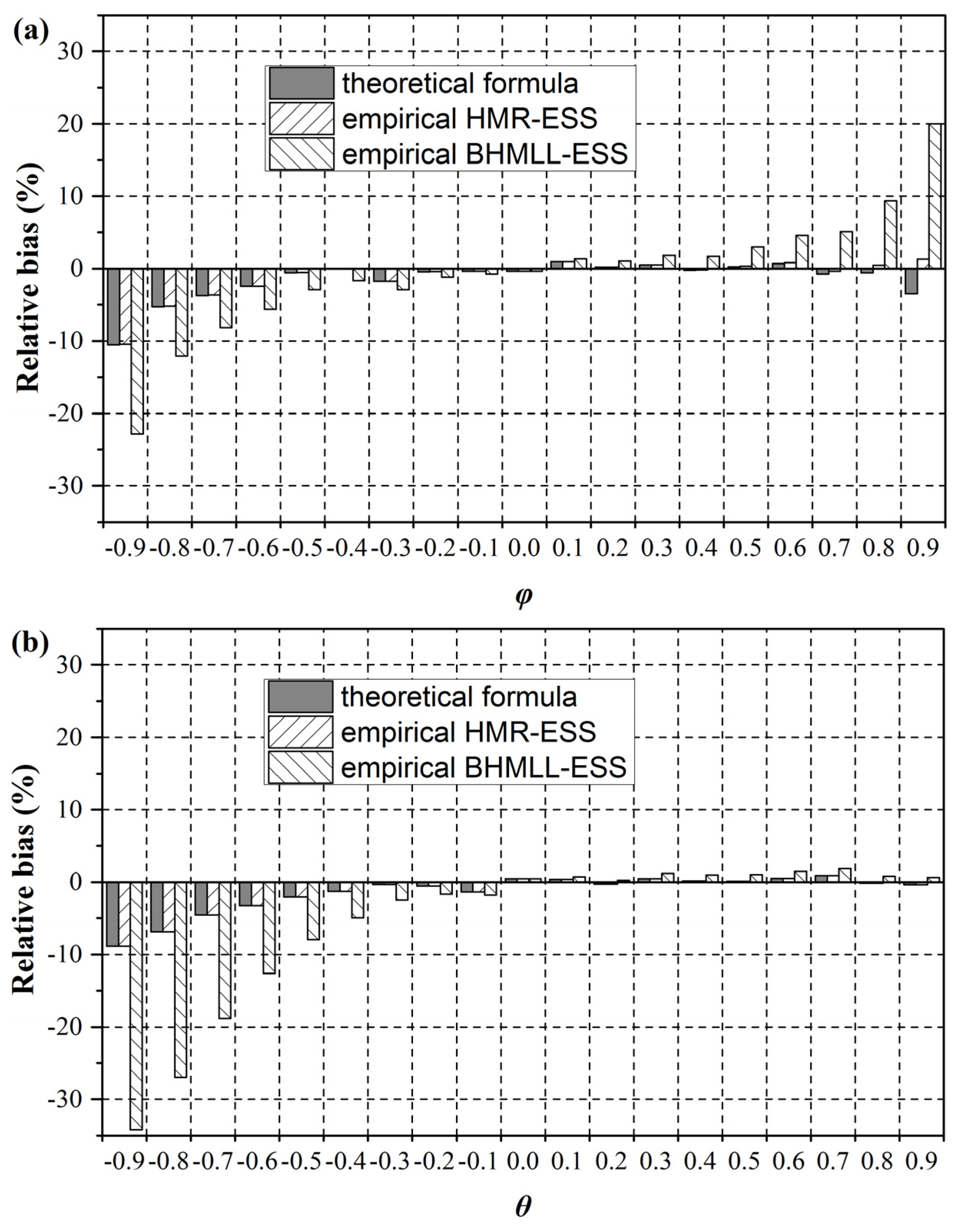
The use of empirical formulae and unavoidable sampling errors of the r(i) estimation interfere with Type І errors and the power of the VC-SR test. In order to highlight this influence, we discuss simulation results based on three cases. In the first case, we apply the theoretical formula with a pre-known autocorrelation structure. Every lag of data autocorrelation coefficients r(i) is calculated based on the specific autocorrelation function. The test is denoted by VC-SR^Theo.. For the second case, we substitute the empirical formula for the theoretical one, and refer to the test as the VC-SR^{ESS+Theo. r} test. We also apply the empirical formula for the third case; however, we follow the procedure that only significant r(i) are estimated from the detrended series and the initial r(1) estimator are bias corrected. The test is referred as VC-SR^{ESS+Est. r}.

For comparison, we also apply the SR test combined with PW, TFPW, and BBS approaches to each simulated series and investigate their ability to correct Type І errors and power.

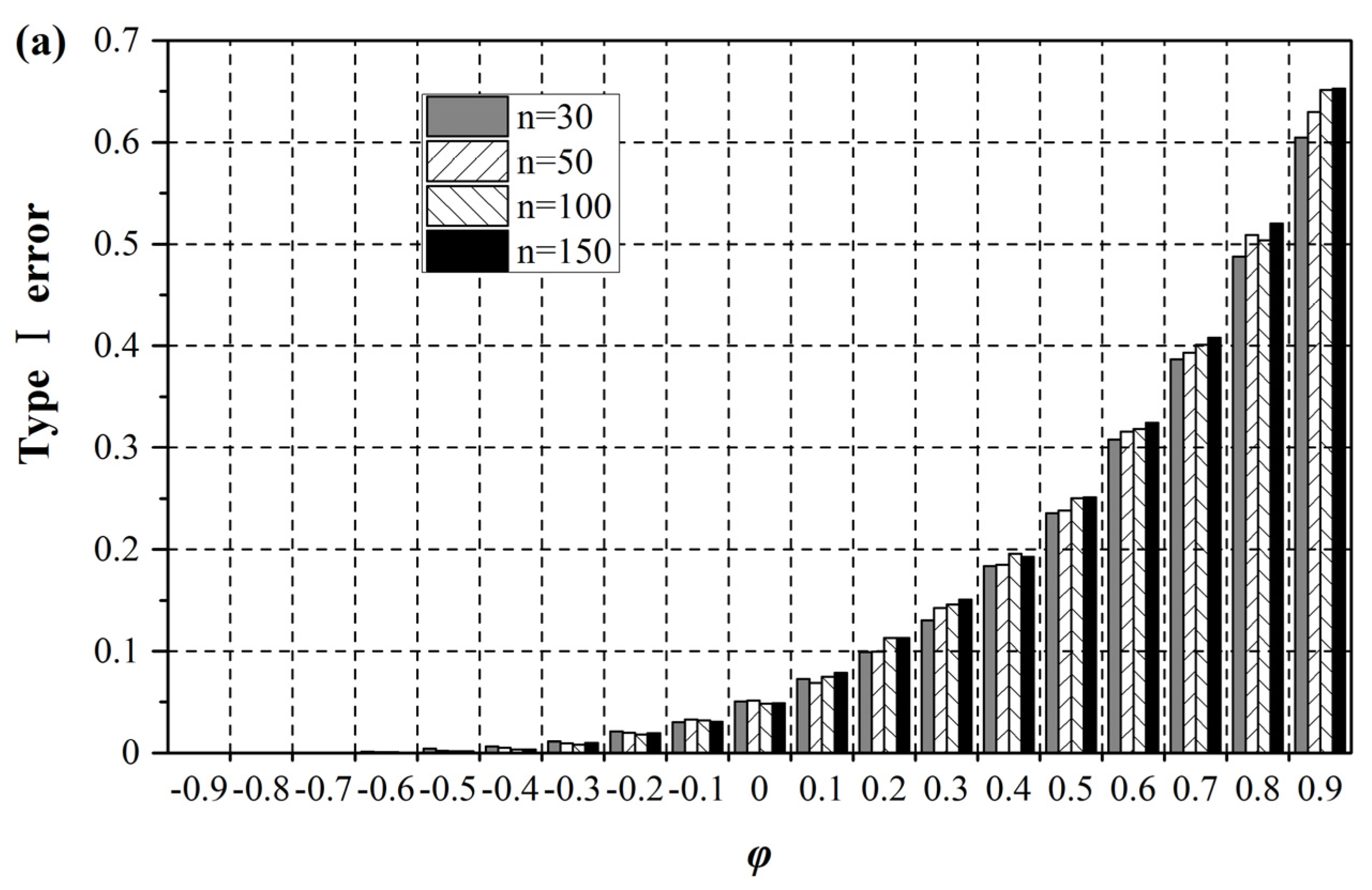
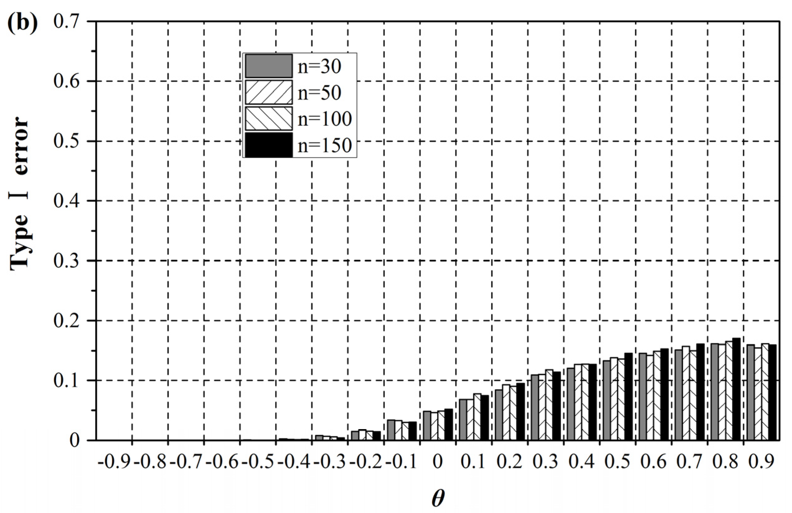
4.2. Type І Error Correction

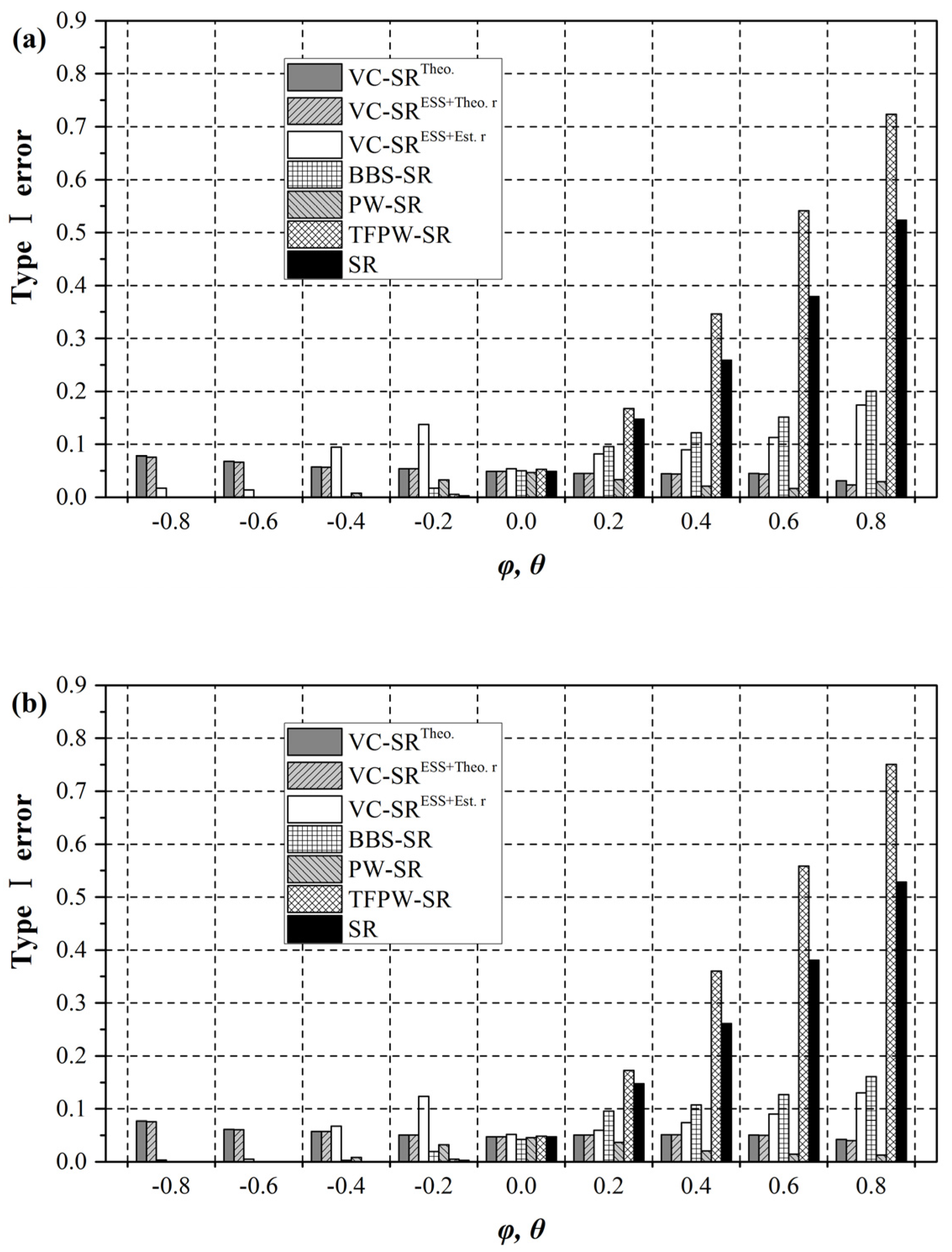
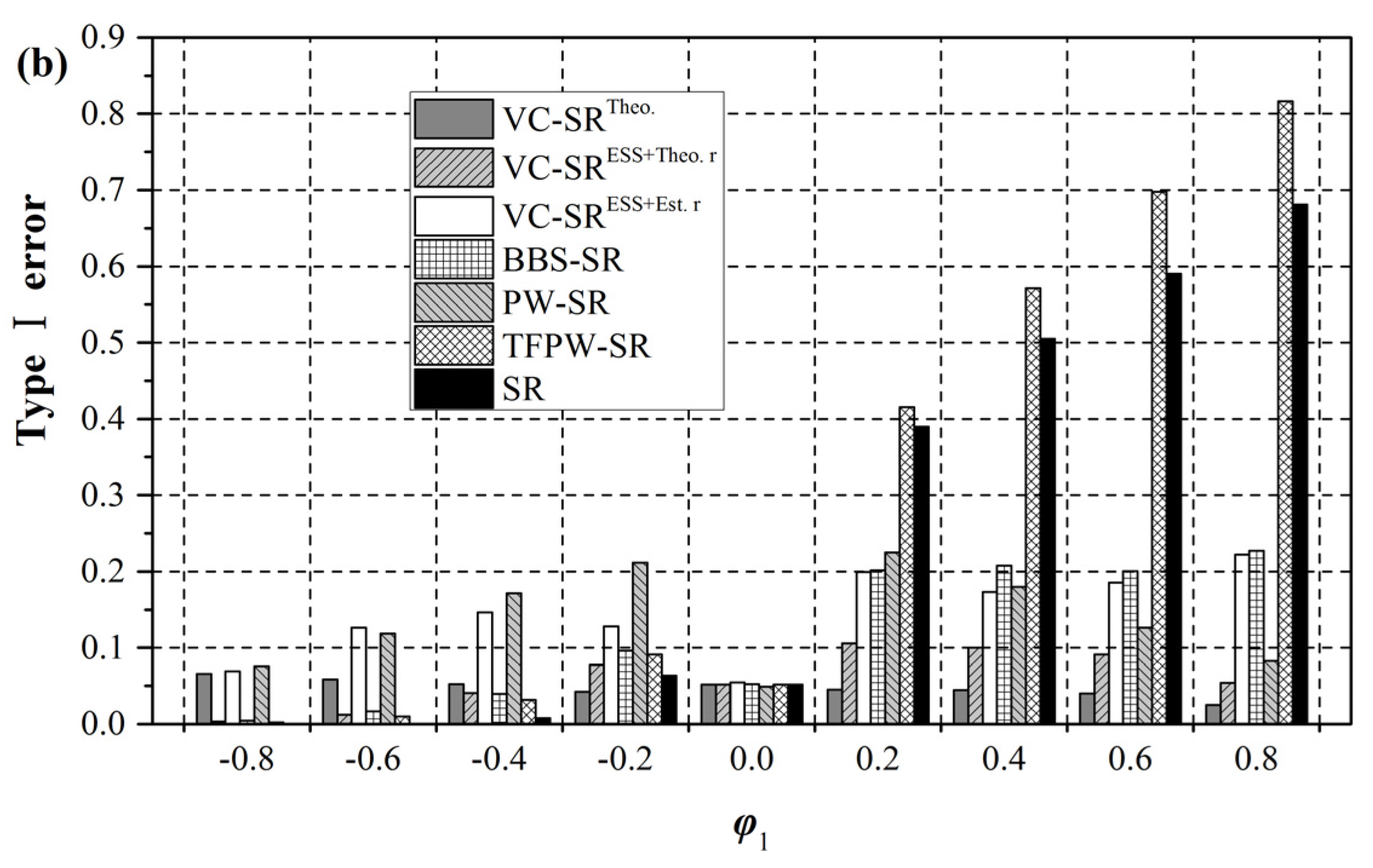
As expected (Figure 5 and Figure 6), the VC-SR^Theo. test, to a large extent, restores the inflationary (deflationary) Type І errors to a value close to 0.05. The use of the empirical formula does not change Type І errors considerably. The VC-SR^{ESS+Theo. r} test yields almost the same results as the VC-SR^Theo. test for the ARMA(1,1) model. It slightly raises Type І errors to around 0.10 in the case of positive autocorrelation for the AR(2) model. 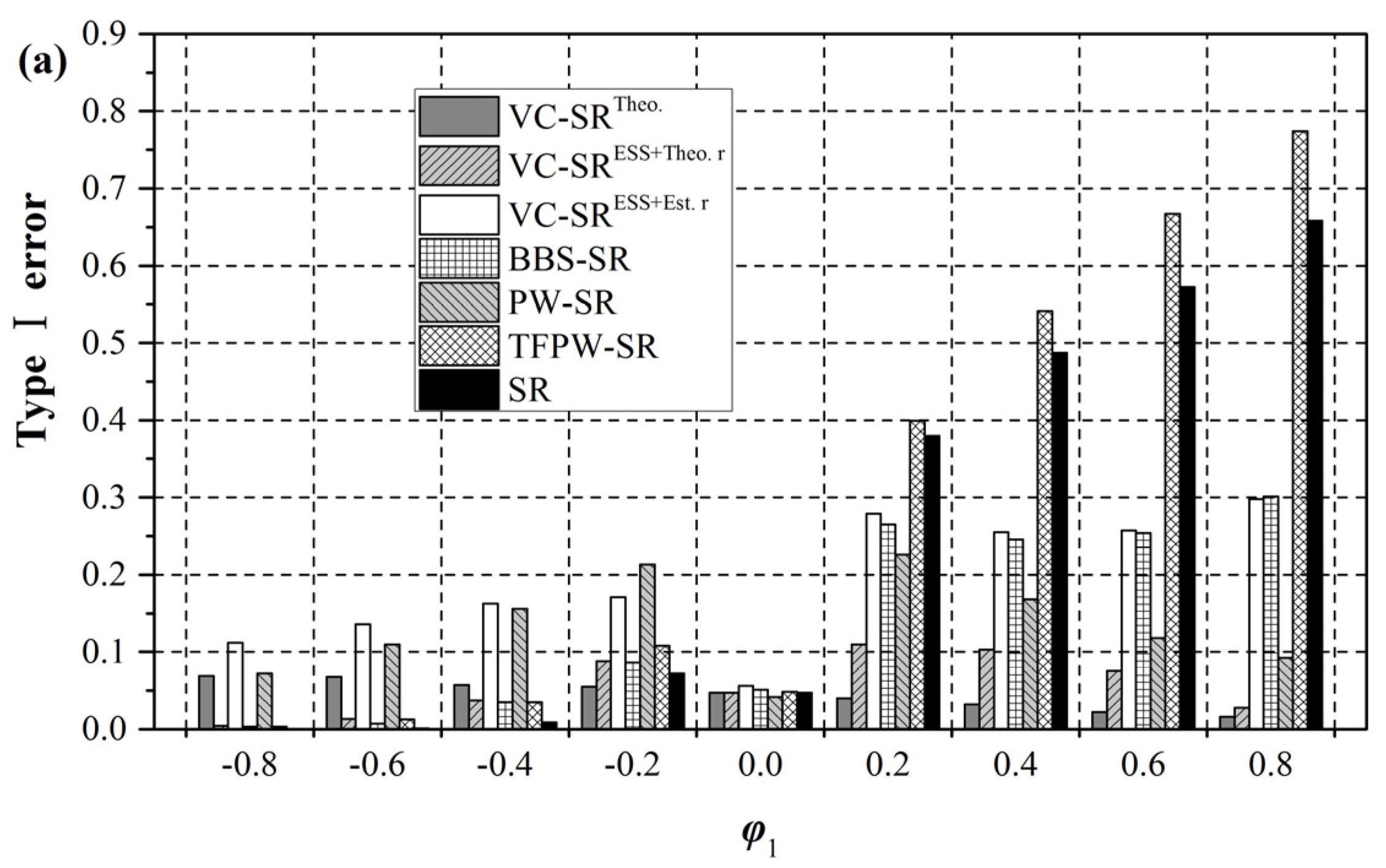Under the influence of sampling errors, the VC-SR^{ESS+Est. r} test loses some abilities: its Type І errors slightly increase with the increasing autocorrelation. It nevertheless presents a notable effectiveness in mitigating the effect of autocorrelation. For ARMA(1,1) series with small sample sizes (n = 50) and positive autocorrelation, the test reduces the Type І errors of the original SR test from the range (0.15–0.50) to (0.08–0.17). Larger sample sizes (compare n = 100 with n = 50) can further enhance this ability. The BBS-SR test bears some resemblance to the VC-SR^{ESS+Est. r} test.

Figure 5. Comparison of Type І errors of different Spearman Rho (SR) tests for ARMA(1,1) series: (a) n = 50; (b) n = 100.

Figure 5. Comparison of Type І errors of different Spearman Rho (SR) tests for ARMA(1,1) series: (a) n = 50; (b) n = 100.

Figure 6. Comparison of Type І errors of different SR tests for AR(2) series: (a) n = 50; (b) n = 100.

Figure 6. Comparison of Type І errors of different SR tests for AR(2) series: (a) n = 50; (b) n = 100.

The PW-SR test, which is AR(1)-based in this case, yields systematic under- and over-rejection for the ARMA(1,1) and AR(2) model, respectively. This problem is mostly related to the model misspecification. Indeed, the ARMA(1,1)- or AR(2)-based PW approach will perfectly preserve stable Type І errors as similar to the VC-SR^Theo. test. Nevertheless, even a slight change in the model structure would interfere with its ideal performance. We take the ARMA(1,1) model as an instance. The AR(1) based approach whitens the series according to the r(1) estimator of the ARMA(1,1) model. Since parameters φ and θ of the ARMA(1,1) model have been designed to change simultaneously from −0.8 to 0.8 as stated above, we may yield

$$\frac{{\mathsf{\phi }}^{\mathrm{A}\mathrm{R}\left(1\right)}}{{\mathsf{\phi }}^{\mathrm{ARMA}}}=\frac{\mathrm{r}{\left(1\right)}^{\mathrm{ARMA}}}{{\mathsf{\phi }}^{\mathrm{ARMA}}}=\frac{2{\mathsf{\phi }}^{\mathrm{ARMA}}\left[1+{\left({\mathsf{\phi }}^{\mathrm{ARMA}}\right)}^2\right]}{1+3{\left({\mathsf{\phi }}^{\mathrm{ARMA}}\right)}^2}\times \frac{1}{{\mathsf{\phi }}^{\mathrm{ARMA}}}=1+\frac{1-{\left({\mathsf{\phi }}^{\mathrm{ARMA}}\right)}^2}{1+3{\left({\mathsf{\phi }}^{\mathrm{ARMA}}\right)}^2}>1$$

(20)

That means the AR(1)-based approach tends to over-whiten series generated from the ARMA(1,1) model, which can explain the under-rejection behavior depicted in Figure 5. Detailed results of the influence of the chosen model on the effectiveness of the PW approach can be taken from Hamed [19].

The TFPW-SR test yields very high Type І errors, which are, in fact, even higher than those of the original SR test. This will result in an unexpectedly high probability of detecting non-existent trends. One reasonable explanation is that the variance of the slope estimator is also inflated by the positive autocorrelation. Even in the case of stationary series, we will falsely report a considerable number of nonzero slopes. To reinstall these spurious trends to the pre-whitened series is obviously detrimental to obtaining correct Type І errors. Another explanation attributes the inflationary Type І errors to the deflationary variance of residuals after whitening the series. By addressing at least one of these reasons we expect to effectively restore Type І errors [24,25,26].

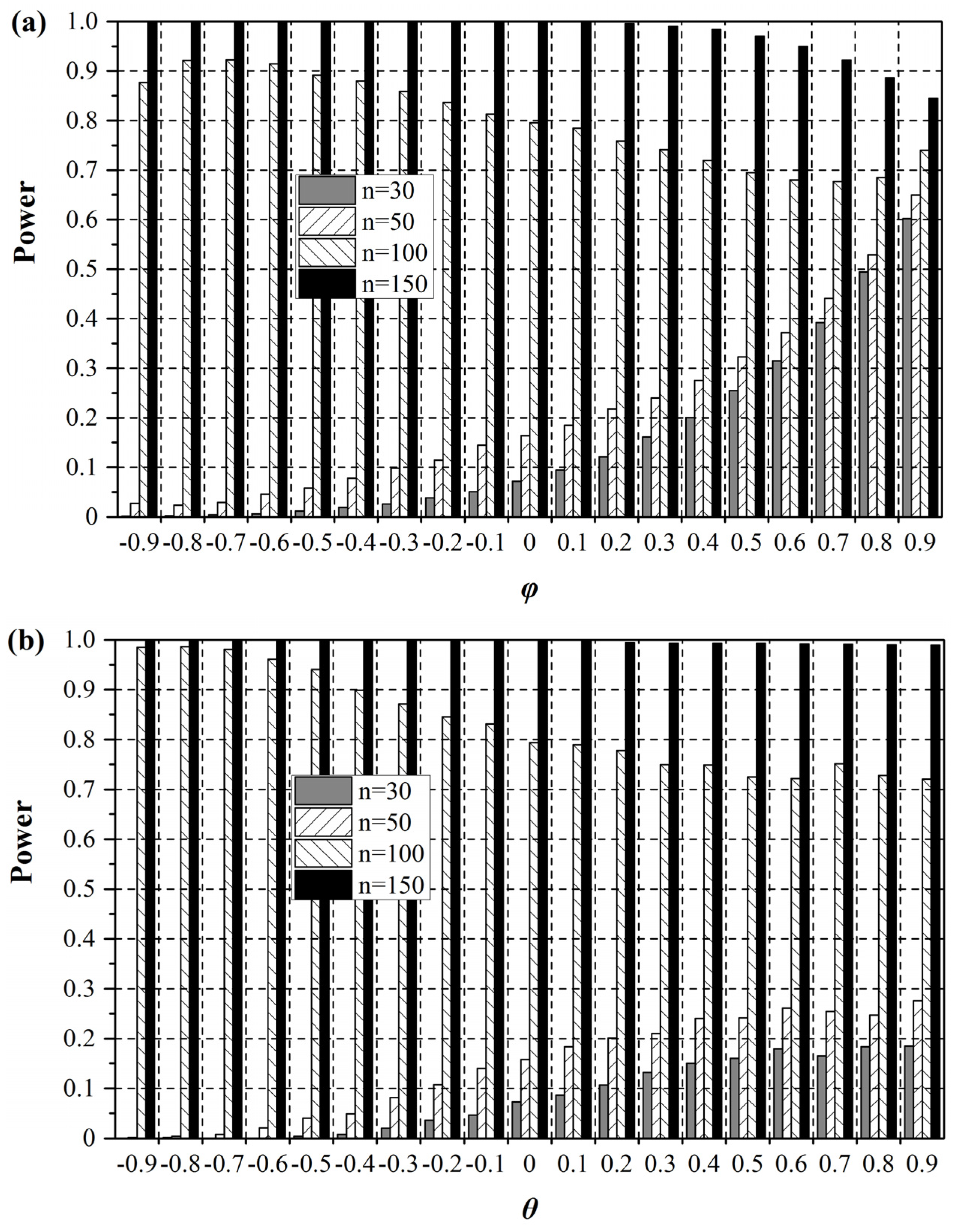
4.3. Power Correction

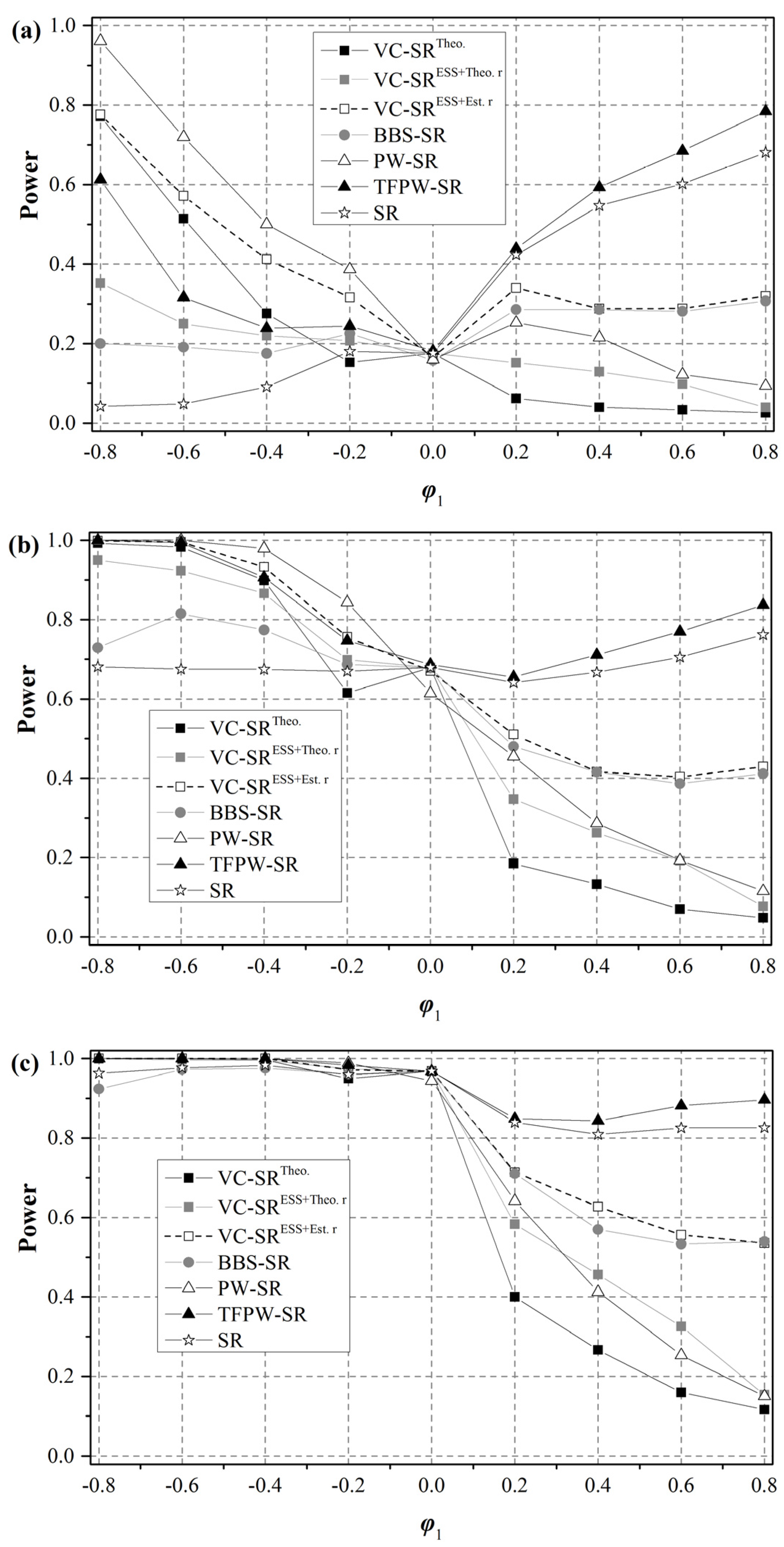
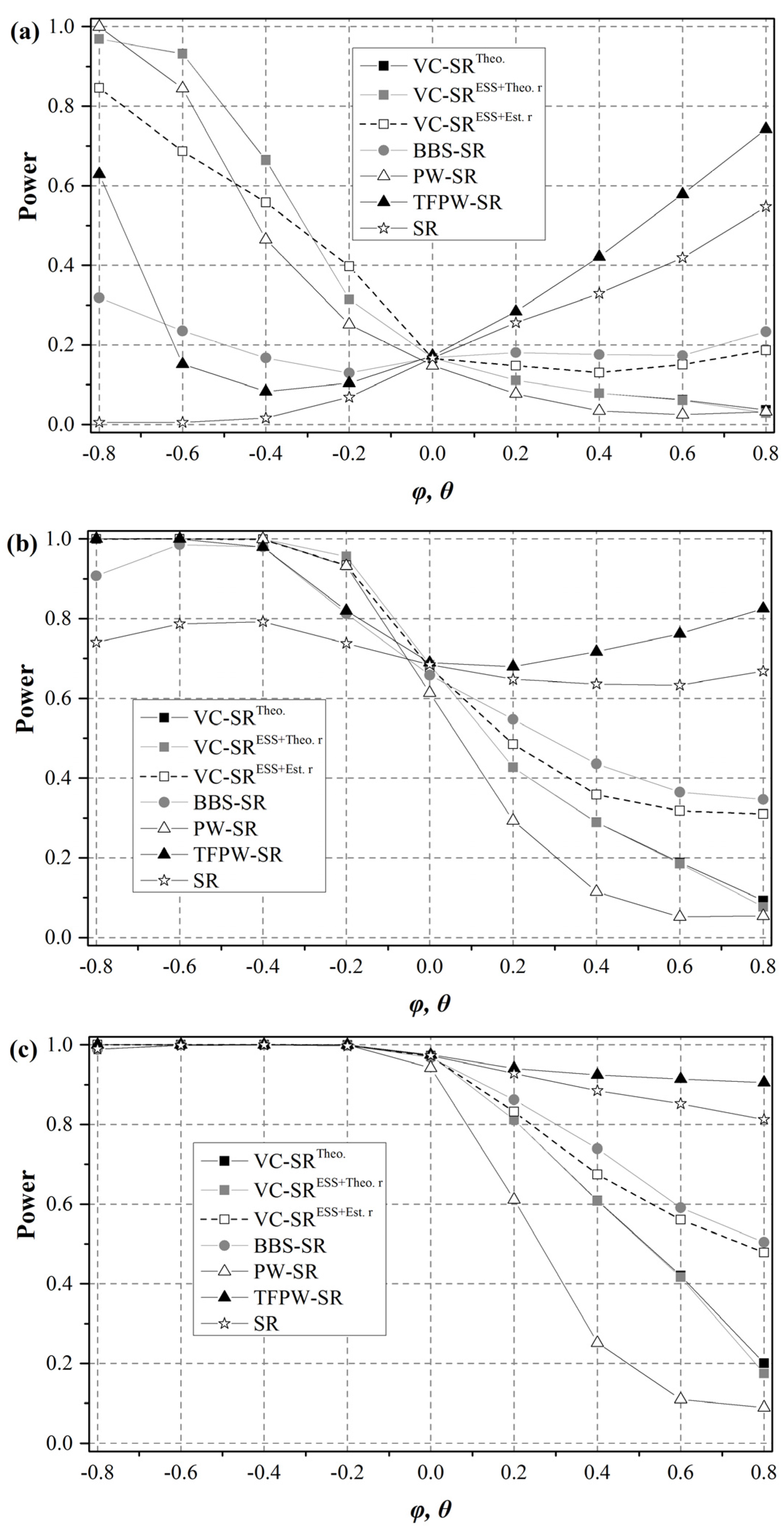
In terms of power (Figure 7 and Figure 8), all SR tests show similar power for independent data ($\mathsf{\phi },\mathsf{\theta },{\mathsf{\phi }}_1=0$); however, their performances with serially dependent data differ considerably. The power of the VC-SR test and the PW-SR test decrease with increasing autocorrelation. The TFPW-SR test performs similarly to the original SR test, as their powers fluctuate as the autocorrelation increases. Their power values increase for series with the weak trends but decrease for series with steep trends. The BBS-SR test is almost unaffected by autocorrelation when trends are weak ($\mathsf{\beta }=0.002$).

Given that hydrometeorological series are often positively autocorrelated, the VC-SR^Theo., the VC-SR^{ESS+Theo. r} and the PW-SR test always rank among all tests with the lowest power. Their ability to detect a real trend will rapidly decrease as the autocorrelation increases. For example, the probability of identifying a significant trend is less than 20% when the slope of the real trend is steep ($\mathsf{\beta }=0.008$) and the autocorrelation is strong ($\mathsf{\phi },\mathsf{\theta },{\mathsf{\phi }}_1=0.8$). Although the TFPW-SR test is the most powerful test, its Type І errors deviate considerably from the pre-assigned significance level, which makes its high power questionable. The powers of the VC-SR^{ESS+Est. r} and the BBS-SR test are comparable; their performance is somewhat average when compared to other tests. For series with steep trends, their powers are no less than 50%, even in the case of the strongest autocorrelation.

In light of both Type І errors and power results, we conclude that even though no single test can thoroughly eliminate the effect of autocorrelation, the VC-SR^{ESS+Est. r} and the BBS-SR test are practical choices since they are capable of keeping relatively accurate Type І errors without significantly losing power.

Figure 7. Comparison of the power of different SR tests for ARMA(1,1) series (n = 50): (a) β = 0.002; (b) β = 0.005; (c) β = 0.008.

Figure 7. Comparison of the power of different SR tests for ARMA(1,1) series (n = 50): (a) β = 0.002; (b) β = 0.005; (c) β = 0.008.

Figure 8. Comparison of power of different SR tests for AR(2) series (n = 50): (a) β = 0.002; (b) β = 0.005; (c) β = 0.008.

Figure 8. Comparison of power of different SR tests for AR(2) series (n = 50): (a) β = 0.002; (b) β = 0.005; (c) β = 0.008.

5. Application

We compare the performance of different SR tests based on annual mean potential evapotranspiration records (PET) within the upper Yangtze River basin, which is one of the major water and hydropower sources of China. 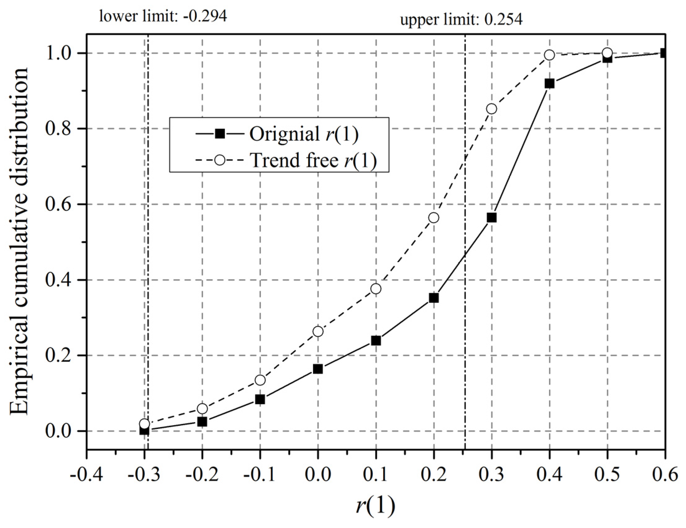Continuous annual series from 1961 to 2011 are available at 372 grid points (0.5° spatial resolution) provided by the Climate Research Unit, University of East Anglia (CRU TS 3.22 dataset) [40]. The analysis of serial dependence reveals that approximately 58% and 28% of grid points yield significantly positive r(1) values based on the original series and detrended series, respectively (Figure 9). We therefore expect trend detection results at these grids and statements regarding their spatial distribution to be affected by autocorrelation.

Figure 9. The empirical cumulative distribution of r(1) values estimated from potential evapotranspiration (PET) data.

Figure 9. The empirical cumulative distribution of r(1) values estimated from potential evapotranspiration (PET) data.

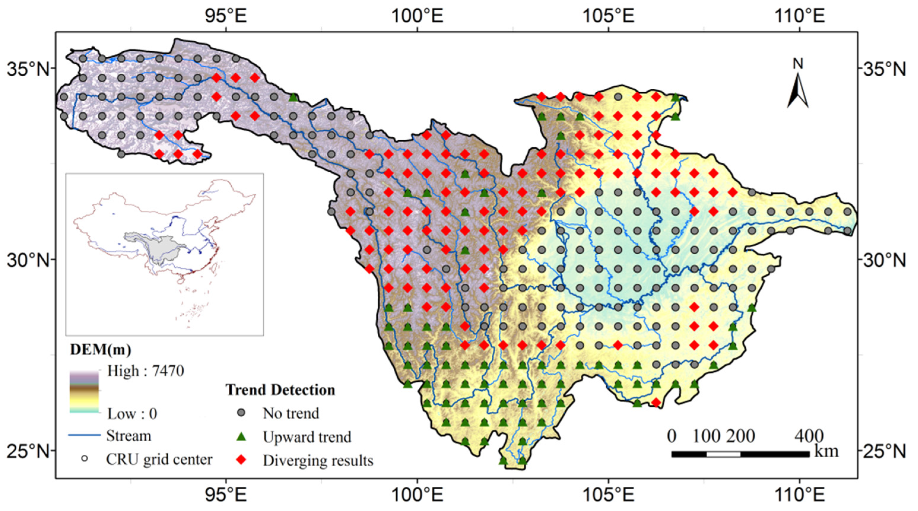
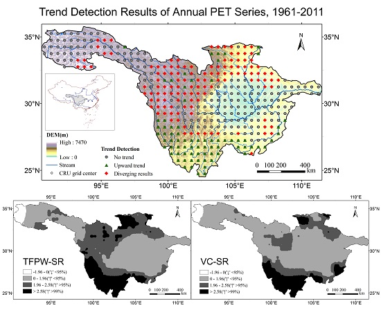
At the significance level of 0.05, the original SR test suggests that 174 grid points, accounting for 47% of the total grid points, exhibit significant upward trends. However, this number is greatly reduced to 75 (20%) if we require all SR tests to be in agreement. As illustrated in Figure 10, most of the grid points with positive trends are located in the southern region of the basin. Applying various SR tests yields diverging results for 125 (34%) grid points, most of which are located in the northern part of the basin between 98° E and 108° E. The other 172 (46%) grid points, statistically, have not changed beyond natural variability.

Figure 10. Trend detection results of annual mean PET data (1961–2011) in the upper Yangtze River basin.

Figure 10. Trend detection results of annual mean PET data (1961–2011) in the upper Yangtze River basin.

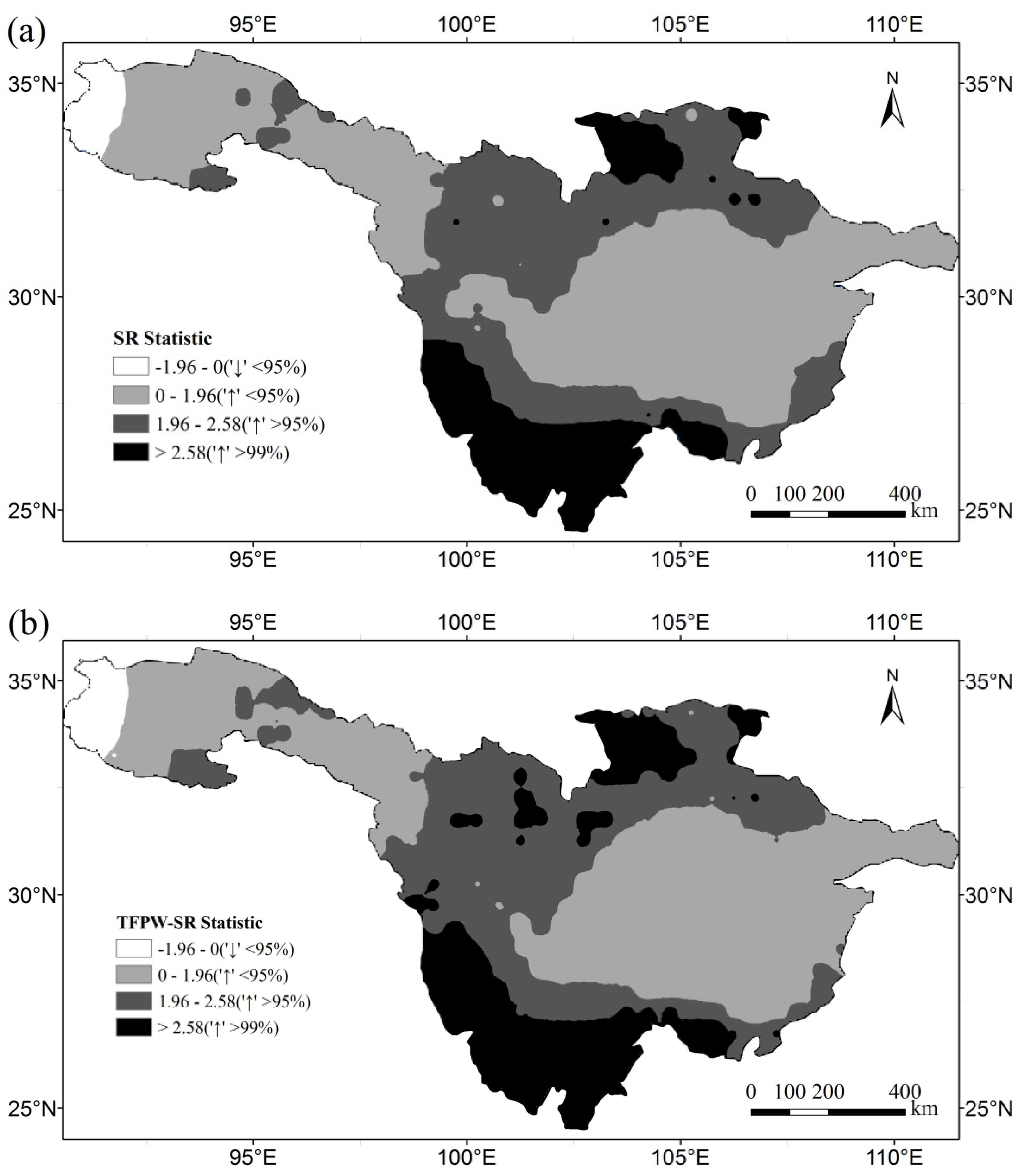
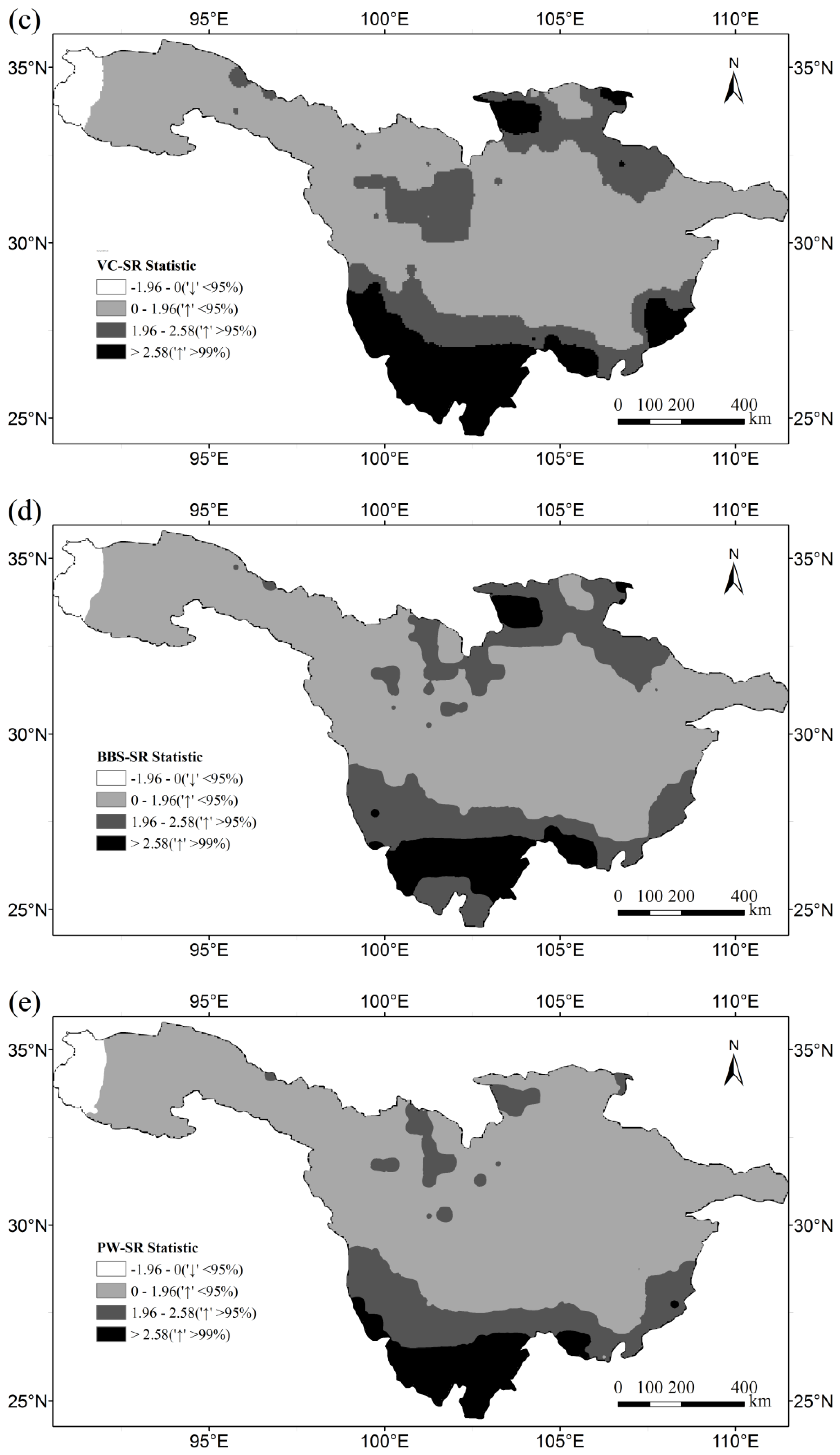
The different power of each test can be verified by observing the spatial distribution of trend detection results (Figure 11). Clearly, the TFPW approach does not substantially correct the results of the original SR test. In fact, it even overestimates the significance of upward trends in some areas. All other tests mitigate the inflationary significance due to positive autocorrelation more effectively. The PW-SR test rejects the existence of trends for most grid points while the VC-SR^{ESS+Est. r} and the BBS-SR tests yield similar results. The latter suggests that the northern region of the basin between 103° E and 108° E experienced positive trends.

Figure 11. Spatial distribution of trend detection results of PET data: (a) the original SR test; (b) the TFPW-SR test; (c) the VC-SR^{ESS+Est. r} test; (d) the BBS-SR test; (e) the PW-SR test.

Figure 11. Spatial distribution of trend detection results of PET data: (a) the original SR test; (b) the TFPW-SR test; (c) the VC-SR^{ESS+Est. r} test; (d) the BBS-SR test; (e) the PW-SR test.

6. Limitations

We need to emphasize that applying the proposed procedure of the VC-SR test with confidence requires that autocorrelation is limited to short term persistence (STP). Some case studies demonstrated that accounting for long term persistence (LTP) would decrease the number of significant trends detected under the assumption of STP [9,41]. If LTP (including trend-like change) is a possible explanation for natural variability, we may resort to scaling stochastic processes; for example, fractional Gaussian noise model (FGN) or fractionally differenced autoregressive integrated moving average model (FARIMA) to represent the series [42,43]. In that case, other parameters, such as the Hurst exponent and the fractional order of differencing, have to be incorporated into the r(i) estimators. This will introduce additional sampling errors of estimation. The VC-SR test cannot be readily utilized for long-term persistent data unless these sampling errors are properly dealt with and the normality of the Spearman rho is verified. Based on stochastic simulation results of FGN, Hamed [33] provided an empirical expression to correct the bias of rho variance due to sampling errors of the Hurst exponent. Furthermore, the exact distribution of Spearman rho converges on the normal distribution in an acceptable manner, although the speed of convergence, in terms of the increasing sample size, is slower than for other trend test statistics, such as Kendall’s tau. Further studies are needed to address Type І errors and the power of the VC-SR test to assess the significance of trends in different scaling stochastic processes and to provide a practical procedure to differentiate LTP from STP.

Another challenge is related to the fact that hydrometeorological variables commonly deviate from normal distributions. The null hypothesis of the original SR test is distributional free, implying that its Type І errors are independent from the data skewness. It is reasonable to infer that the VC-SR test inherits this merit since it does not impose an additional distributional assumption. However, the data skewness does change the power of the test. Yue [2] found that the MK test is more likely to detect significant trends in variables if they are following Pearson Type III or extreme value distributions rather than normal distributions. If this finding is valid for the VC-SR test, the test would probably achieve higher power than that shown in the current simulation results, which are generated from a normal distribution.

7. Conclusions

Our study addresses the influence of autocorrelation on trend analyses, which is often overlooked in the interpretation of the possible significant trends versus natural random variability. To mitigate this adverse influence, we developed the Variance Correction Spearman Rho Trend Test. It consists of two major efforts. Firstly, we derived a theoretical formula to calculate the rho variance that can account for every lag of data autocorrelation coefficients. Compared with the earlier expression for the same purpose, the new formula can save around 75% of computation time. Both formulae share similar accuracy in calculating rho variance under the influence of autocorrelation for large sample sizes. Secondly, we provide a practical procedure to implement variance correction that only requires significant lags. Statistical simulation results confirm the satisfactory performance of the proposed method. It ultimately yields acceptable Type І errors and maintains a relatively strong power of trend detection. This ability bears much resemblance to the Block Bootstrap method.

Among other techniques, the TFPW approach tends to inflate Type І errors excessively and is not recommended for serially dependent data. The PW approach is more effective for the correction of Type І errors and is still a practical choice for trend detection. Users, however, should notice that its capability is sensitive to model misspecifications if the series are whitened by a parametric autocorrelation model. Furthermore, the PW approach is actually assessing the significance of deflated trend slopes.

We conclude that neglecting the effect of autocorrelation or dealing with it without choosing adequate methods will lead to incorrect results. A first step of a robust trend detection strategy would be an evaluation of regional characteristics of observations. A second step would lead to selecting methods with acceptable Type І errors and power, based on a well-tailored simulation study. A final step would include a comparison of results of various methods and an interpretation of plausible underlying physical mechanisms. The proposed VC-SR test is one meaningful option to implement this strategy.

References

1. Kendall, M.G. Rank Correlation Methods; Charles Griffin: London, UK, 1955; Chapter 5. [Google Scholar]
2. Yue, S.; Pilon, P.; Cavadias, G. Power of the Mann-Kendall and Spearman’s rho tests for detecting monotonic trends in hydrological series. J. Hydrol. 2002, 259, 254–271. [Google Scholar] [CrossRef]
3. Talaee, P.H. Iranian rainfall series analysis by means of nonparametric tests. Theor. Appl. Climatol. 2013, 116, 597–607. [Google Scholar] [CrossRef]
4. Burn, D.H.; Elnur, M.A.H. Detection of hydrologic trends and variability. J. Hydrol. 2002, 255, 107–122. [Google Scholar] [CrossRef]
5. Kundzewicz, Z.W. Searching for change in hydrological data. Hydrol. Sci. J. 2004, 49, 3–6. [Google Scholar] [CrossRef]
6. Kundzewicz, Z.W.; Graczyk, D.; Maurer, T.; Pińskwar, I.; Radziejewski, M.; Svensson, C.; Szwed, M. Trend detection in river flow series: 1. Annual maximum flow. Hydrol. Sci. J. 2005, 50, 797–810. [Google Scholar] [CrossRef]
7. Svensson, C.; Kundzewicz, W.Z.; Maurer, T. Trend detection in river flow series: 2. Flood and low-flow index series. Hydrol. Sci. J. 2005, 50, 811–824. [Google Scholar] [CrossRef]
8. Zhang, Q.; Peng, J.; Xu, C.Y.; Singh, V.P. Spatiotemporal variations of precipitation regimes across Yangtze river basin, China. Theor. Appl. Climatol. 2013, 115, 703–712. [Google Scholar] [CrossRef]
9. Khaliq, M.N.; Ouarda, T.B.M.J.; Gachon, P.; Sushama, L. Temporal evolution of low-flow regimes in Canadian rivers. Water Resour. Res. 2008, 44. [Google Scholar] [CrossRef]
10. Narayanan, P.; Basistha, A.; Sarkar, S.; Sachdeva, K. Trend analysis and ARIMA modelling of pre-monsoon rainfall data for western India. Comptes Rendus Geosci. 2013, 345, 22–27. [Google Scholar] [CrossRef]
11. Zhang, X.; Vincent, L.A.; Hogg, W.D.; Niitsoo, A. Temperature and precipitation trends in Canada during the 20th century. Atmos. Ocean 2000, 38, 395–429. [Google Scholar] [CrossRef]
12. Liuzzo, L.; Bono, E.; Sammartano, V.; Freni, G. Analysis of spatial and temporal rainfall trends in Sicily during the 1921–2012 period. Theor. Appl. Climatol. 2015. [Google Scholar] [CrossRef]
13. Kundzewicz, Z.W.; Robson, A.J. Change detection in hydrological records-a review of the methodology. Hydrol. Sci. J. 2004, 49, 7–19. [Google Scholar] [CrossRef]
14. Khaliq, M.N.; Ouarda, T.B.M.J.; Gachon, P.; Sushama, L.; St-Hilaire, A. Identification of hydrological trends in the presence of serial and cross correlations: A review of selected methods and their application to annual flow regimes of Canadian rivers. J. Hydrol. 2009, 368, 117–130. [Google Scholar] [CrossRef]
15. Sonali, P.; Kumar, D.N. Review of trend detection methods and their application to detect temperature changes in india. J. Hydrol. 2013, 476, 212–227. [Google Scholar] [CrossRef]
16. Von Storch, H. Misuses of Statistical Analysis in Climate Research; Springer-Verlag: Berlin, Germany, 1995. [Google Scholar]
17. Yue, S.; Wang, C.Y. Applicability of prewhitening to eliminate the influence of serial correlation on the Mann-Kendall test. Water Resour. Res. 2002, 38, 1068. [Google Scholar] [CrossRef]
18. Bayazit, M.; Önöz, B. To prewhiten or not to prewhiten in trend analysis? Hydrol. Sci. J. 2007, 52, 611–624. [Google Scholar] [CrossRef]
19. Hamed, K.H. Enhancing the effectiveness of prewhitening in trend analysis of hydrologic data. J. Hydrol. 2009, 368, 143–155. [Google Scholar] [CrossRef]
20. Yue, S.; Pilon, P. Canadian streamflow trend detection-impacts of serial and cross-correlation. Hydrol. Sci. J. 2003, 48, 51–63. [Google Scholar] [CrossRef]
21. Yue, S.; Pilon, P.; Phinney, B.; Cavadias, G. The influence of autocorrelation on the ability to detect trend in hydrological series. Hydrol. Process. 2002, 16, 1807–1829. [Google Scholar] [CrossRef]
22. Rivard, C.; Vigneault, H. Trend detection in hydrological series: When series are negatively correlated. Hydrol. Process. 2009, 23, 2737–2743. [Google Scholar] [CrossRef]
23. Blain, G.C. The Mann-Kendall test the need to consider the interaction between serial correlation and trend. Acta Sci. Agron. 2013, 36, 393–402. [Google Scholar]
24. Zhang, X.B.; Zwiers, F.W. Comment on “Applicability of prewhitening to eliminate the influence of serial correlation on the Mann-Kendall test” by Sheng Yue and Chun Yuan Wang. Water Resour. Res. 2004, 40, 1–5. [Google Scholar] [CrossRef]
25. Serinaldi, F.; Kilsby, G.C. The importance of prewhitening in change point analysis under persistence. Stoch. Environ. Res. Risk Assess. 2015. [Google Scholar] [CrossRef]
26. Wang, W.; Chen, Y.; Becker, S.; Liu, B. Variance correction prewhitening method for trend detection in autocorrelated data. J. Hydrol. Eng. 2015, 12, 04015033. [Google Scholar] [CrossRef]
27. Önöz, B.; Bayazit, M. Block bootstrap for Mann-Kendall trend test of serially dependent data. Hydrol. Process. 2012, 26, 3552–3560. [Google Scholar] [CrossRef]
28. Radziejewski, M.; Bardossy, A.; Kundzewicz, Z.W. Detection of change in river flow using phase randomization. Hydrol. Sci. J. 2000, 45, 547–558. [Google Scholar] [CrossRef]
29. Franzke, C. A novel method to test for significant trends in extreme values in serially dependent time series. Geophys. Res. Lett. 2013, 40, 1391–1395. [Google Scholar] [CrossRef]
30. Noguchi, K.; Gel, Y.R.; Duguay, C.R. Bootstrap-based tests for trends in hydrological time series, with application to ice phenology data. J. Hydrol. 2011, 410, 150–161. [Google Scholar] [CrossRef]
31. Hamed, K.H.; Rao, A.R. A modified Mann-Kendall trend test for autocorrelated data. J. Hydrol. 1998, 204, 182–196. [Google Scholar] [CrossRef]
32. Hamed, K.H. Trend detection in hydrologic data: The Mann-Kendall trend test under the scaling hypothesis. J. Hydrol. 2008, 349, 350–363. [Google Scholar] [CrossRef]
33. Hamed, K.H. The distribution of Spearman’s rho trend statistic for persistent hydrologic data. Hydrol. Sci. J. 2014. [CrossRef]
34. Matalas, N.C.; Sankarasubramanian, A. Effect of persistence on trend detection via regression. Water Resour. Res. 2003, 39, SWC 7.1–SWC 7.7. [Google Scholar] [CrossRef]
35. Bayley, G.V.; Hammersley, J.M. The effective number of independent observations in an autocorrelated time series. J. R. Stat. Soc. 1946, 8, 184–197. [Google Scholar] [CrossRef]
36. Lettenmaier, D.P. Detection of trends in water quality data from records with dependent observations. Water Resour. Res. 1976, 12, 1037–1046. [Google Scholar] [CrossRef]
37. Yue, S.; Wang, C. The Mann-Kendall test modified by effective sample size to detect trend in serially correlated hydrological series. Water Resour. Manag. 2004, 18, 201–218. [Google Scholar] [CrossRef]
38. Sen, P.K. Estimates of the regression coefficient based on kendall’s tau. J. Am. Stat. Assoc. 1968, 63, 1379–1389. [Google Scholar] [CrossRef]
39. Salas, J.D. Analysis and modeling of hydrologic time series. In Handbook of Hydrology; Maidment, D., Ed.; McGraw-Hill: New York, NY, USA, 1993; Chapter 19; pp. 19.1–19.72. [Google Scholar]
40. Harris, I.; Jones, P.D.; Osborn, T.J.; Lister, D.H. Updated high-resolution grids of monthly climatic observations—The CRU TS3.10 Dataset. Int. J. Climatol. 2014, 34, 623–642. [Google Scholar] [CrossRef] [Green Version]
41. Cohn, T.A.; Lins, H.F. Nature’s style: Naturally trendy. Geophys. Res. Lett. 2005, 32. [Google Scholar] [CrossRef]
42. Koutsoyiannis, D. The hurst phenomenon and fractional gaussian noise made easy. Hydrol. Sci. J. 2002, 47, 573–595. [Google Scholar] [CrossRef]
43. Montanari, A.; Rosso, R.; Taqqu, M.S. Fractionally differenced ARIMA models applied to hydrologic time series: Identification, estimation, and simulation. Water Resour. Res. 1997, 33, 1035–1044. [Google Scholar] [CrossRef]